Grlweap frank rausche

GRLWEAP - Santa Cruz, 20151

Congreso Internacional de Fundaciones Profundas de Bolivia

Santa Cruz, Bolivia, 12 al 15 de Mayo de 2015

Day 1: Software DemonstrationsFrank Rausche, Ph.D., P.E., D.GE - Pile Dynamics, Inc.

Applications of Stress Wave Theory to Deep Foundations with an Emphasis on

“The Wave Equation”(GRLWEAP)


CONTENTCONTENT

• Introduction– Dynamic Formula

– Static Formula

• The One‐Dimensional Wave Equation and Wave Demonstrations

• Wave Equation Models

• Bearing Graph and Driveability

• Example

• Conclusions


WAVE EQUATION OBJECTIVESWAVE EQUATION OBJECTIVES

Smith’s Basic Interest:

– Allow for realistic stress calculations– Replace Unreliable Energy Formulas– Use improved models

• elastic pile• elasto‐plastic static resistance• viscous dynamic (damping) resistance • detailed driving system representation


Wave Demonstrations

– Slinky

– Pendulum

– Buddies

– Shear Waves

– Compressive Waves


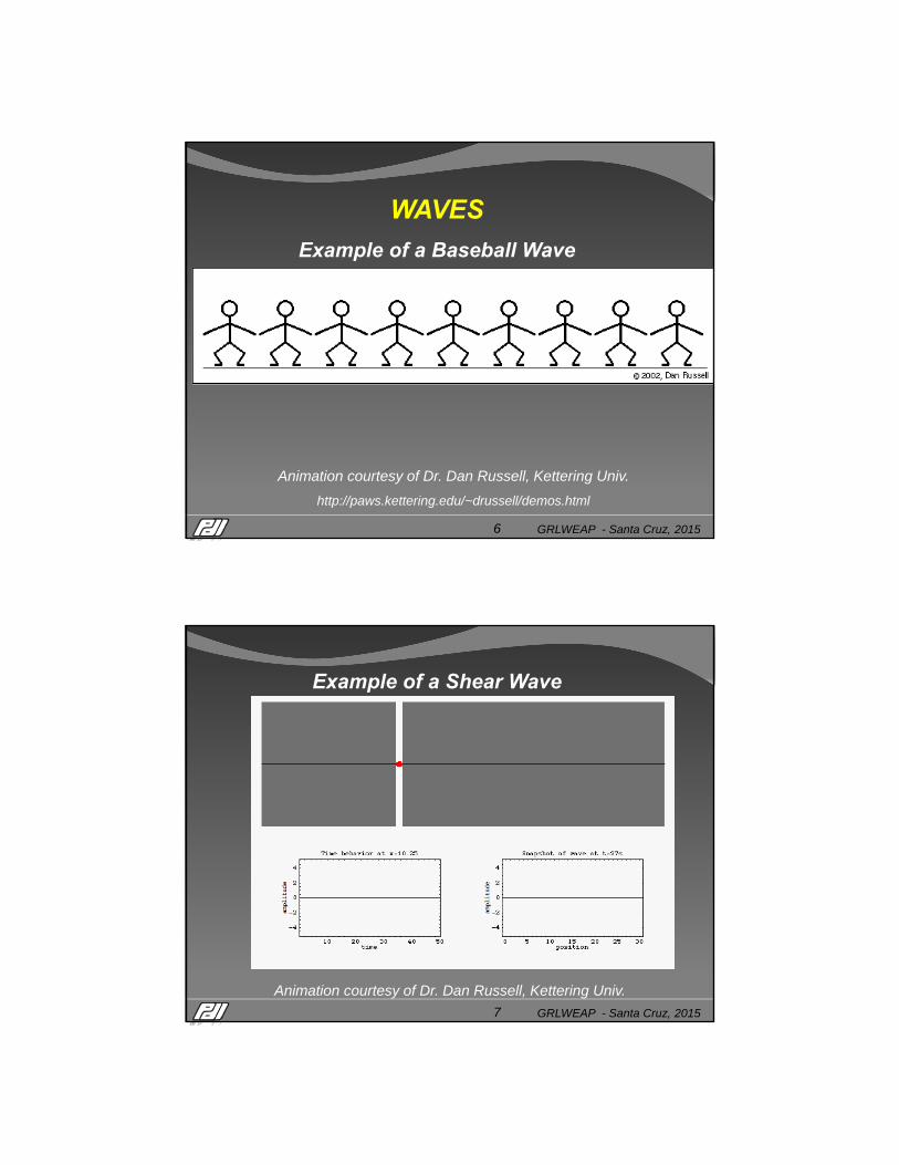
Animation courtesy of Dr. Dan Russell, Kettering Univ.

http://paws.kettering.edu/~drussell/demos.html

WAVES

Example of a Baseball Wave



Example of a Shear Wave



Example of a Compressive Wave


The 1-D Wave Equation

ρ(δ2u/ δt2) = E (δ2u/ δx2)E … elastic modulus

ρ … mass density

with c2 = E/ ρ ... Wave Speed

Solution: u = f(x‐ct) + g(x+ct)

x … length coordinate

t ... time

u … displacement

f

gx


x

Timet

The compression wave,induced by the

hammer at the pile top, moves downward a

distance c t during the time interval t.

Waves in a PileWaves in a Pile


x

Timet t + t

C t

The compression wave, induced by the hammer at the pile top, moves

downward a distance c t during the time

interval t.

Waves in a PileWaves in a Pile


The compression wave, arrives at the pile toe where it

is reflected(on a free pile in tension).

t Time t + t Waves in a Pile


2012 13 Wave Mechanics for Pile Testers

x

u

ρ(δ2u/ δt2) = E (δ2u/ δx2)

E … elastic modulus

ρ … mass density

with c2 = E/ ρ … Wave Speed

x … length coordinate t ... time

u … displacement

THE Wave Equation

Solution: u = f(x-ct) + g(x+ct)


2012 14 Wave Mechanics for Pile Testers

f

g

x

f

g

x

C t

C t

Time

t + tTime

t

The Solution to the Wave Equationu = f(x-ct) + g(x+ct)


Force, F – Time to + t

Point A

Point A, like all other points along the pile, is at rest at time to (when

contact between ram and pile top occurs)

Compressed distance, L

Time to

u

The first instant after impact


∆u is the displacement of a point of pile during time ∆t

F

∆L

Wave travels distance ∆L = c ∆t during time ∆t

Particle Velocity, v = ∆u/ ∆t but ∆u = ε ∆L and therefore v = ε ∆L / ∆t and with wave speed c = ∆L / ∆t:

∆u

Force Velocity ProportionalityForce Velocity Proportionality

v = ε c


This is the strain, stress, force-velocity proportionality

Z = EA/c is the pile impedance (kN/m/s)

This is the strain, stress, force-velocity proportionality

Z = EA/c is the pile impedance (kN/m/s)

Fd = vd (EA/c)Fd = vd (EA/c)

d = vd(E/c)d = vd(E/c)εd = vd / cεd = vd / c

Strain-Stress-Force ProportionalityWave travels in one direction only

Strain-Stress-Force ProportionalityWave travels in one direction only


Express Your ImpedanceExpress Your Impedance

Z = EA/c kN/(m/s)

with c = (E/ρ)1/2 Z = A (E ρ)1/2

with E = c2 ρ Z = A c ρ

with Mp= L A ρ Z = Mp c/ L (Mp ... pile mass)

The Pile Impedance is a force which changes the pile velocity suddenly by 1 m/s.

Reversely, if the velocity changes by 1 m/s then pile will develop a force equal to Z.


A Quick Look at Energy FormulasA Quick Look at Energy Formulas

Energy Dissipated in Soil =

Energy Provided by Hammer

Ru (s + sl) = ηWrh

sl … “lost” set (empirical or measured),

η … efficiency of hammer/driving system

Engineering News: Rallow = Wr h / 6(s + 0.1)


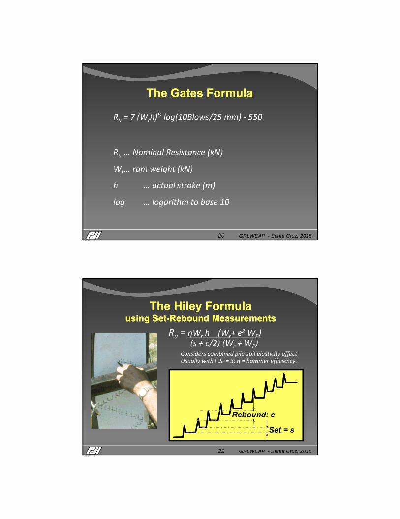
The Gates Formula The Gates Formula

Ru = 7 (Wrh)½ log(10Blows/25 mm) ‐ 550

Ru … Nominal Resistance (kN)

Wr… ram weight (kN)

h … actual stroke (m)

log … logarithm to base 10


The Hiley Formulausing Set-Rebound Measurements

The Hiley Formulausing Set-Rebound Measurements

Ru = ηWr h (Wr+ e2 WP)

(s + c/2) (Wr + WP)

Rebound: c

Set = s

Considers combined pile‐soil elasticity effectUsually with F.S. = 3; η = hammer efficiency.


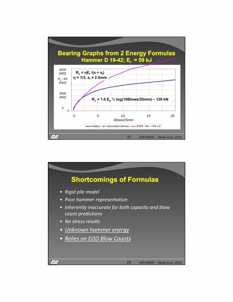
Bearing Graphs from 2 Energy FormulasHammer D 19-42; Er = 59 kJ

Bearing Graphs from 2 Energy FormulasHammer D 19-42; Er = 59 kJ

0

500

1000

1500

2000

2500

3000

3500

4000

0 25 50 75 100 125 150 175 200

Blows/0.25 m

Capacity in

kN

Gates - w/ calculated Stroke ENR - Ru = Rd x 2

Ru = ηEr /(s + sl)η = 1/3; sl = 2.5mm

Ru = 1.6 Ep ½ log(10Blows/25mm) – 120 kN

4000[900]

Ru - kN[kips]

2000[450]

0

0 5 10 15 20Blows/25mm


Shortcomings of FormulasShortcomings of Formulas

• Rigid pile model

• Poor hammer representation

• Inherently inaccurate for both capacity and blow count predictions

• No stress results

• Unknown hammer energy

• Relies on EOD Blow Counts


Static FormulasStatic Formulas

• Based on Soil Properties

• Always done for any deep foundation type

• Backed up by Static or Dynamic Testing


Static Analysis to Calculate LTSR

Basically for All Soil Types:

Ru = Ru,shaft + Ru,toeRu = fsAs + qt At

fs, Ru,shaft, As … Shaft Resistance/Area

qt, Ru,toe, At … End Bearing/Area


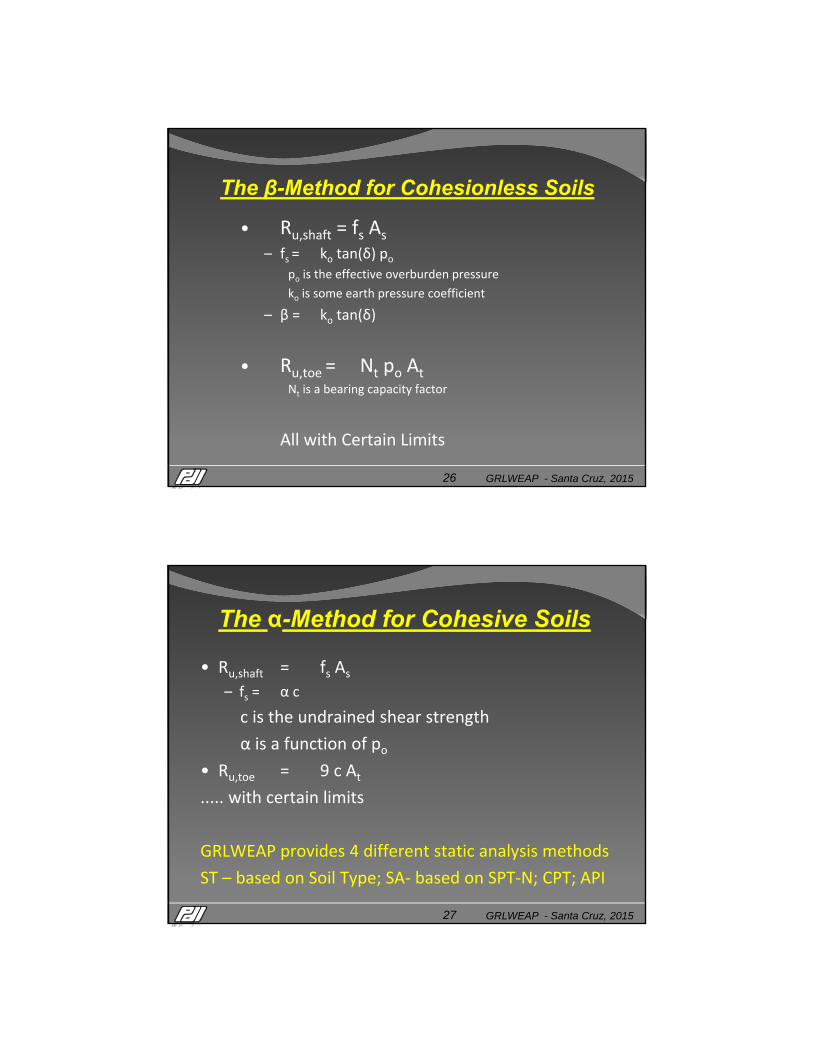
The β-Method for Cohesionless Soils

• Ru,shaft = fs As

– fs = ko tan(δ) popo is the effective overburden pressure

ko is some earth pressure coefficient

– β = ko tan(δ)

• Ru,toe = Nt po AtNt is a bearing capacity factor

All with Certain Limits


The α-Method for Cohesive Soils

• Ru,shaft = fs As

– fs = α c

c is the undrained shear strength

α is a function of po• Ru,toe = 9 c At

..... with certain limits

GRLWEAP provides 4 different static analysis methods

ST – based on Soil Type; SA‐ based on SPT‐N; CPT; API


GRLWEAP: ST MethodNon-Cohesive Soils (after Bowles)

Soil Parameters in ST Analysis for Granular Soil Types

Soil Type SPT NFriction Angle

Unit Weight, γ β Nt Limit (kPa)

degrees kN/m3 Qs Qt

Very loose 2 25 - 30 13.5 0.203 12.1 24 2400

Loose 7 27 - 32 16 0.242 18.1 48 4800

Medium 20 30 - 35 18.5 0.313 33.2 72 7200

Dense 40 35 - 40 19.5 0.483 86.0 96 9600

Very Dense 50+ 38 - 43 22 0.627 147.0 192 19000


ST - INPUTST - INPUT


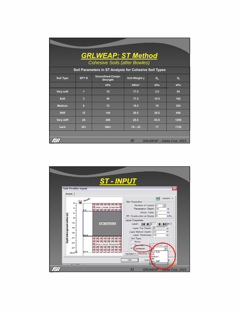
GRLWEAP: ST MethodCohesive Soils (after Bowles)

Soil Parameters in ST Analysis for Cohesive Soil Types

Soil Type SPT NUnconfined Compr.

StrengthUnit Weight γ Qs Qt

kPa kN/m3 kPa kPa

Very soft 1 12 17.5 3.5 54

Soft 3 36 17.5 10.5 162

Medium 6 72 18.5 19 324

Stiff 12 144 20.5 38.5 648

Very stiff 24 288 20.5 63.5 1296

hard 32+ 384+ 19 – 22 77 1728


ST - INPUTST - INPUT


The Wave Equation ModelThe Wave Equation Model

• The Wave Equation Analysis calculates– The displacement of any point along a slender, elastic rod at any time durting and after impact

– From the displacements forces, stresses, velocities

• The calculation is based on rod properties: – Length

– Cross Sectional Area

– Elastic Modulus

– Mass density


The Wave Equation ModelThe Wave Equation Model

• The Wave Equation Analysis calculates– The displacement of any point along a slender, elastic rod at any time durting and after impact

– From the displacements forces, stresses, velocities

• The calculation is based on rod properties: – Length

– Cross Sectional Area

– Elastic Modulus

– Mass density


GRLWEAP FundamentalsGRLWEAP Fundamentals

• For a pile driving analysis, the “slender, elastic rod” consists of Hammer+DrivingSystem+Pile

• The soil is represented by resistance forces acting on the pile and representing the forces in the pile‐soil interface

Ham

mer

D.S.

Pil

e


Smith’s Numerical Solution of the Wave EquationSmith’s Numerical Solution of the Wave Equation

∆L

ρ(δ2u/ δt2) = E (δ2u/ δx2)E … elastic modulus ‐ ρ … mass densitywith c2 = E/ ρ ... Wave Speed

Closed Form Solutions to the wave equation are not practical; we therefore solve the equation numerically:

(mi/ki)(ui,j+1 ‐2ui,j + ui,j‐1)/Δt2

= (ui+1,j – 2ui,j + ui‐1,j)

This is equivalent to considering mass points and springs!

ii+1

i-1


The GRLWEAP Pile ModelThe GRLWEAP Pile Model

Each segment has a mass and spring stiffness

– of length ∆L ≤ 1 m (3.3 ft)

– with mass m = ρ A ∆L

– and stiffness k = E A / ∆L

there are N = L / ∆L pile segments which allow us to solve the wave equation numerically.

∆L


The Pile ModelThe Pile Model

Relationship between the uniform pile and the

lumped mass model properties:

m k = (ρ A ∆L)(EA/∆L) = A2Eρ = Z2 [kN s/m]2

m/k = (ρ A ∆L)/(EA/∆L) = (ρ/E)∆L2 = (∆L/c)2 [s]2

Or

Z = (mk)1/2 (pile impedance) and

∆t = (m/k)1/2 (wave travel time)

Note: the smaller ∆L, the smaller ∆L and that means the higher the frequencies that can be

represented.

∆L


We can model 3 hammer-pile systemsWe can model 3 hammer-pile systems


Ram: A, L for stiffness, mass

Cylinder and upper frame = assembly top mass

Drop height

External Combustion Hammer Modeling

Ram guides for assembly stiffness

Hammer base = assembly bottom mass


External Combustion Hammer ModelExternal Combustion Hammer Model

• Ram modeled like rod

• Stroke is an input (Energy/Ram Weight)

• Impact Velocity Calculated from Stroke with Hammer Efficiency Reduction: vi = (2 g h η) ½

• Assembly also modeled because it may impact during pile rebound

• Note approximation in data file:

Assembly mass = Total hammer mass – Ram mass


External Combustion HammersRam Model

Ram segments ~1m long

Combined Ram‐H.Cushion

Helmet mass


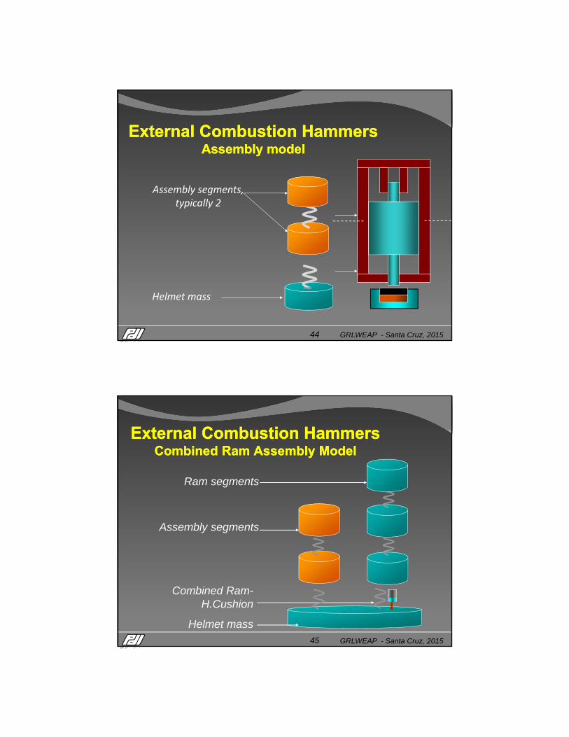
External Combustion HammersAssembly model

External Combustion HammersAssembly model

Assembly segments, typically 2

Helmet mass


External Combustion HammersCombined Ram Assembly Model

External Combustion HammersCombined Ram Assembly Model

Combined Ram-H.Cushion

Helmet mass

Ram segments

Assembly segments


External Combustion HammerAnalysis Procedure

• Static equilibrium analysis

• Dynamic analysis starts when ram is within 1 ms of

impact.

• All ram segments then have velocity

VRAM = (2 g h η)1/2 – 0.001 g

g is the gravitational acceleration

h is the equivalent hammer stroke and η is the hammer efficiency

h = Hammer potential energy/ Ram weight


• Dynamic analysis ends when

– Pile toe has rebounded to 80% of max dtoe

– Pile has penetrated more than 4 inches

– Pile toe has rebounded to 98% of max dtoe and energy

in pile is essentially dissipated

External Combustion HammerAnalysis Procedure


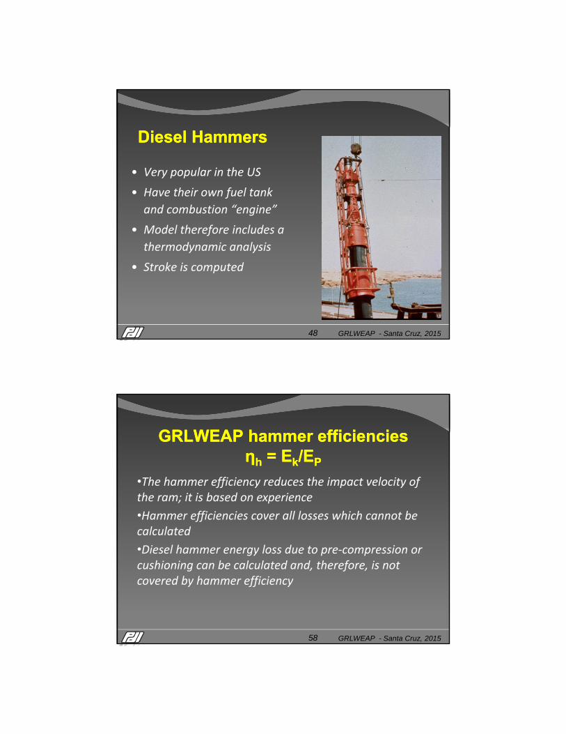
Diesel HammersDiesel Hammers

• Very popular in the US

• Have their own fuel tank

and combustion “engine”

• Model therefore includes a

thermodynamic analysis

• Stroke is computed


GRLWEAP hammer efficienciesηh = Ek/EP

GRLWEAP hammer efficienciesηh = Ek/EP

•The hammer efficiency reduces the impact velocity of the ram; it is based on experience

•Hammer efficiencies cover all losses which cannot be calculated

•Diesel hammer energy loss due to pre‐compression or cushioning can be calculated and, therefore, is not covered by hammer efficiency


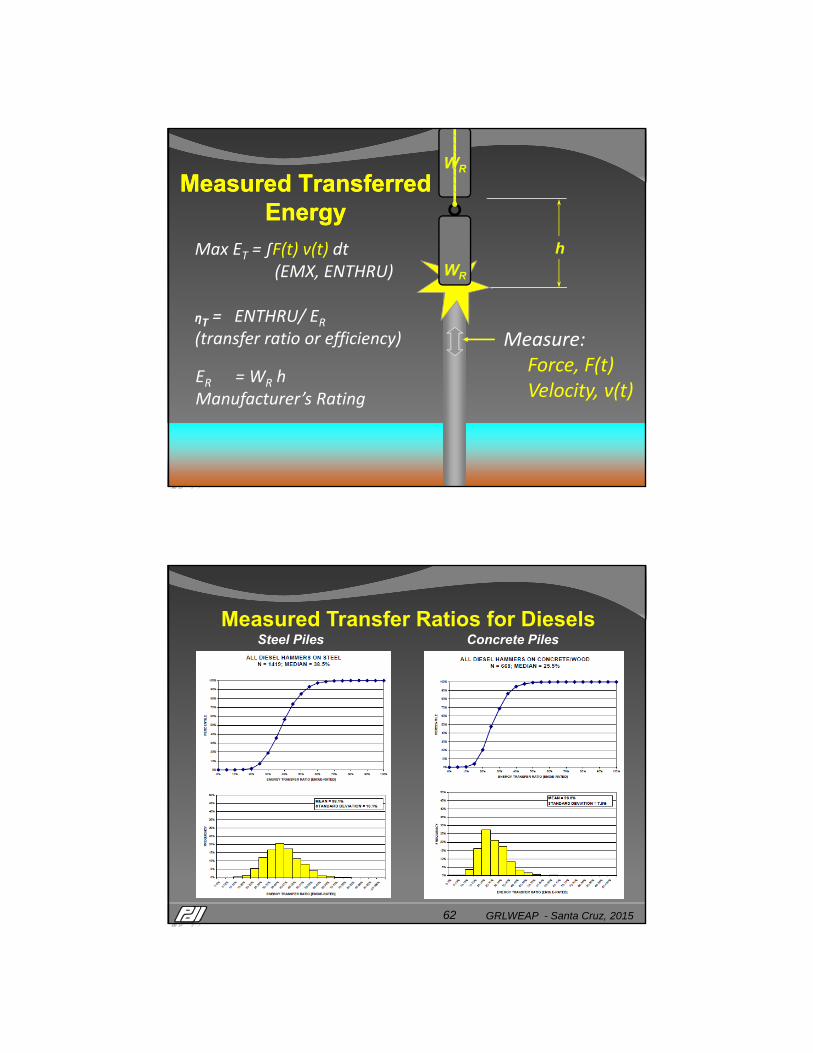
WR

h

ER = WR hManufacturer’s Rating

WR

Max ET = ∫F(t) v(t) dt(EMX, ENTHRU)

ηT = ENTHRU/ ER(transfer ratio or efficiency) Measure:

Force, F(t)Velocity, v(t)

Measured Transferred Energy

Measured Transferred Energy


Measured Transfer Ratios for DieselsSteel Piles Concrete Piles


For all impact hammers GRLWEAP needs impact velocity

WP

mR

hEr = Wr he = mr g he

he = Er / Wr he – equivalent stroke

he = h for single acting hammers

Epr = η Er Wr he (η = Hammer efficiency )

WRvi

Ek = Epr = ηh (½ mr vi2) (kinetic energy)

vi = 2g heηh


GRLWEAP Diesel hammer efficiencies , ηh

GRLWEAP Diesel hammer efficiencies , ηh

Open end diesel hammers: 0.80uncertainty of fall height, friction, alignment

Closed end diesel hammers: 0.80uncertainty of fall height, friction, power assist, alignment


Modern Hydraulic Hammer Efficiencies, ηh

Modern Hydraulic Hammer Efficiencies, ηh

Hammers with internal monitor: 0.95uncertainty of hammer alignment

Hydraulic drop hammers: 0.80uncertainty of fall height, alignment, friction

Power assisted hydraulic hammers: 0.80uncertainty of fall height, alignment, friction, power assist


Vibratory HammersVibratory Hammers


Vibratory Force:

FV = me [ω2resin ω t ‐ a2(t)]

FL

FV

m1

m2

• Line Force

• Bias Mass and

• Oscillator mass, m2

• Eccentric masses, me, radii, re

• Clamp

Vibratory Hammer ModelVibratory Hammer Model


The Driving Systems Consists of1. Helmet including inserts to

align hammer and pile

2. Optionally: Hammer Cushion to protect hammer

3. For Concrete Piles: Softwood Cushion

Driving System ModelsDriving System Models


Helmet + Inserts

Driving System ModelExample of a diesel hammer

on a concrete piles

Driving System ModelExample of a diesel hammer

on a concrete piles

Hammer Cushion: Spring plus Dashpot

Pile Top: Spring + DashpotPile Cushion


Interface Soil: Elasto‐Plastic Springs and Viscous Dashpots

Soil outside of interface: Rigid

The Soil Model After Smith


Soil ResistanceSoil Resistance

• Soil resistance slows pile movement and causes pile rebound

• A very slowly moving pile only encounters static resistance

• A rapidly moving pile also encounters dynamic resistance

• The static resistance to driving (SRD) differs from the soil resistance under static loads


Segment

i

Segment

i‐1

Segment

i+1

Pile‐Soil Interface

Soil Model ParametersSoil Model Parameters

ki,Rui

Ji

RIGID SOIL

ki+1,Rui+1

Ji+1

ki-1,Rui-1

Ji-1


FixedSoil

Smith’s Soil ModelSmith’s Soil Model

Total Soil ResistanceRtotal = Rsi +Rdi

Total Soil ResistanceRtotal = Rsi +Rdi

Displacement uiVelocity vi

Pile

Segment i


The Static Soil ModelThe Static Soil Model


Pile

Segment i

Pile Displacement

Rui

Static Resistance

Rui … ult. resistanceqi … quake

ksi = Rui /qi


Recommended Toe Quakes, qtoeRecommended Toe Quakes, qtoe

0.1” or 2.5 mm forall soil types0.04” or 1 mm for hard rock

qtoe

Static Toe Res.

qtoe Ru,toe

Toe Displacement

D/120 for very dense or hard soilsD/60 for soils which are not very dense or v. hard

Displacement pilesNon‐displacement piles

D


Toe Quake Effect on Blow Count Toe Quake Effect on Blow Count

S200

100

m

610x

12

95 m

Approximatelyy 50% Shaft Resistance

Total No. of Blows: ∞ (qt =D/60); 27,490 (qt=D/120)

0

10

20

30

40

50

60

70

80

90

100

0 200 400 600 800

Dep

th o

f P

ile T

oe

Pen

etra

tio

n -

m

Blow Count - Blows/m

qt = D/60

qt = D/120


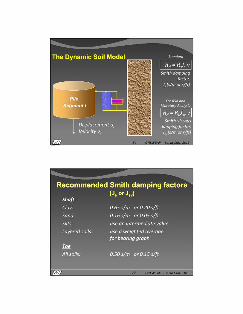
The Dynamic Soil ModelThe Dynamic Soil Model


Pile

Segment i

Rd = RuJsv vSmith‐viscous

damping factor,Jsv [s/m or s/ft]

For RSA and Vibratory Analysis

Smith damping factor,

Js [s/m or s/ft]

Rd = RsJs v

Standard


Recommended Smith damping factors(Js or Jsv)

Recommended Smith damping factors(Js or Jsv)

Shaft

Clay: 0.65 s/m or 0.20 s/ft

Sand: 0.16 s/m or 0.05 s/ft

Silts: use an intermediate value

Layered soils: use a weighted averagefor bearing graph

Toe

All soils: 0.50 s/m or 0.15 s/ft


Shaft Damping on Blow Count Shaft Damping on Blow Count

S200

100

m

610x

12

95 m

Approximatelyy 50% Shaft Resistance

Total No. of Blows: ∞ (Js=0.65 s/m); 27,490 (Js=0.16 s/m)

0

10

20

30

40

50

60

70

80

90

100

0 200 400 600 800

Dep

th o

f P

ile T

oe

Pen

etra

tio

n -

m


Js = 0.65 s/m

Js = 0.16 s/m


GRLWEAP’s Static Analysis MethodsGRLWEAP’s Static Analysis Methods

Rs

Rt

QIcon Input Basic AnalysisST Soil Type Effective Stress, Total StressSA SPT N-value Effective StressCPT R at cone tip and sleeve SchmertmannAPI φ, Su Effective Stress, Total Stress

• GRLWEAP’s static analysis methods may be used for dynamic analysis preparation (resistance distribution, estimate of capacity for driveability).

• For design, be sure to use a method based on local experience.


Use of Static Analysis MethodsUse of Static Analysis Methods

• Should always be done for finding reasonable pile type and length

• For driven piles static analysis is only a starting point, since pile length is determined in the field (exceptions are piles driven to depth, for example, because of high soil setup)

• For LRFD when finding pile length by static analysis method use resistance factor for selected capacity verification method


Resistance DistributionResistance Distribution3. More Involved:

I. ST Input: Soil Type

II. SA Input: SPT Blow Count, Friction Angle or Unconfined Compressive Strength

III. API (offshore wave version) Input: Friction Angle or UndrainedShear Strength

IV. CPT Input: Cone Record including Tip Resistance and Sleeve Friction vs Depth.

Pen

etra

tio

n

All are good for a Bearing GraphII, III and IV OK for Driveability Analysis

Local experience may provide better values


Mass i

Mass i-1

Mass i+1

Numerical TreatmentNumerical Treatment• Predict displacements:

uni = uoi + voi ∆t

Fi, ci

uni-1

uni

uni+1

Ri-1

Ri

Ri+1

• Calculate spring compression:

ci = uni - uni-1

• Calculate spring forces:

Fi = ki ci

• Calculate resistance forces:

Ri = Rsi + Rdi


Force balance at a segmentForce balance at a segment

Acceleration: ai = (Fi + Wi – Ri – Fi+1) / mi

Velocity, vi, and Displacement, ui, from Integration

Mass i

Force from upper spring, Fi

Force from lower spring, Fi+1

Resistance force, Ri Weight, Wi


Set or Blow Count Calculation (a) Simplified: extrapolated toe displacement

Set or Blow Count Calculation (a) Simplified: extrapolated toe displacement

Static soil Resistance

PileDisplacement

Final Set

Max. Displacement

Quake

Ru

Extrapolated

Calculated


Blow Count Calculation(b) Residual Stress Analysis (RSA)

Blow Count Calculation(b) Residual Stress Analysis (RSA)

Set for 2 Blows

Convergence:Consecutive Blows

have same pile compression/sets


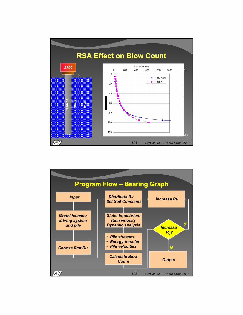
RSA Effect on Blow Count RSA Effect on Blow Count

S500

100

m

1220

x25

0

10

20

30

40

50

60

70

80

90

100

0 200 400 600 800

Dep

th o

f P

ile

To

e P

enet

rati

on

-m


Standard

RSA

95 m

Total No. of Blows: 8907 (Standard); 6235 (RSA)

0

20

40

60

80

100

120

0 200 400 600 800 1000

B lo w C o u n t (b l/m)

No RSA

RSA


Static EquilibriumRam velocity

Dynamic analysis

Program Flow – Bearing GraphProgram Flow – Bearing Graph

Model hammer,driving system

and pile

• Pile stresses• Energy transfer• Pile velocitiesChoose first Ru

Calculate BlowCount

Distribute RuSet Soil Constants

Output

IncreaseRu?

Increase Ru Input

N

Y


Bearing Graph: Variable Capacity, One depthSI-Units; Clay and Sand Example; D19-42; HP 12x53;

Bearing Graph: Variable Capacity, One depthSI-Units; Clay and Sand Example; D19-42; HP 12x53;


Driveability AnalysisDriveability Analysis

• Analyze a series of Bearing Graphs for different depths for SRD and/or LTSR

• Put the results in sequence so that we get predicted blow count and stresses vs pile toe penetration

• Note that, in many or most cases, shaft resistance is lower during driving (soil setup) and end bearing is about the same as long term

• In the few cases of relaxation, the toe resistance is actually higher during driving than long term


Analysis

Program Flow – DriveabilityProgram Flow – Driveability

Model Hammer &Driving System

Choose first Depth to analyze

Next G/L

Pile Length and Model

Calculate Rufor first gain/loss

Output IncreaseDepth?

Increase Depth

Input

IncreaseG/L?

N

N

Y

Y


Driveability Result

During a driving interruption soil setup occurs


When Should we do the Analysis?When Should we do the Analysis?

• Before pile driving begins

– Equipment selection for safe and efficient installation

– Preliminary driving criterion

• After initial pile tests have been done

– Refined Wave Equation analysis for improved driving criterion

– For different driving systems

• In preparation of dynamic testing


SummarySummary• The wave equation analysis simulates what happens in the pile when it is struck by a heavy hammer input.

• It calculates a relationship between capacity and blow count, or blow count vs. depth.

• The analysis model represents hammer (3 types), driving system (cushions, helmet), pile (concrete, steel, timber) and soil (at the pile‐soil interface)

• GRLWEAP provides a variety of input help features (hammer and driving system data, static formulas among others).


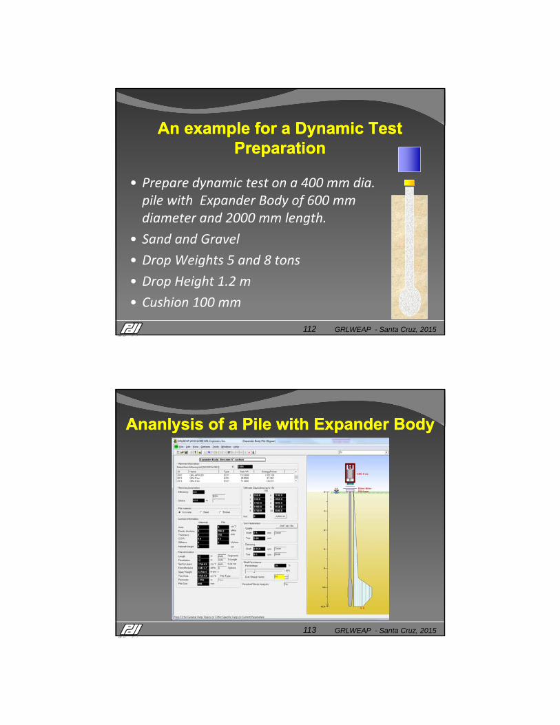
An example for a Dynamic Test Preparation

An example for a Dynamic Test Preparation

• Prepare dynamic test on a 400 mm dia. pile with Expander Body of 600 mm diameter and 2000 mm length.

• Sand and Gravel

• Drop Weights 5 and 8 tons

• Drop Height 1.2 m

• Cushion 100 mm


Ananlysis of a Pile with Expander BodyAnanlysis of a Pile with Expander Body


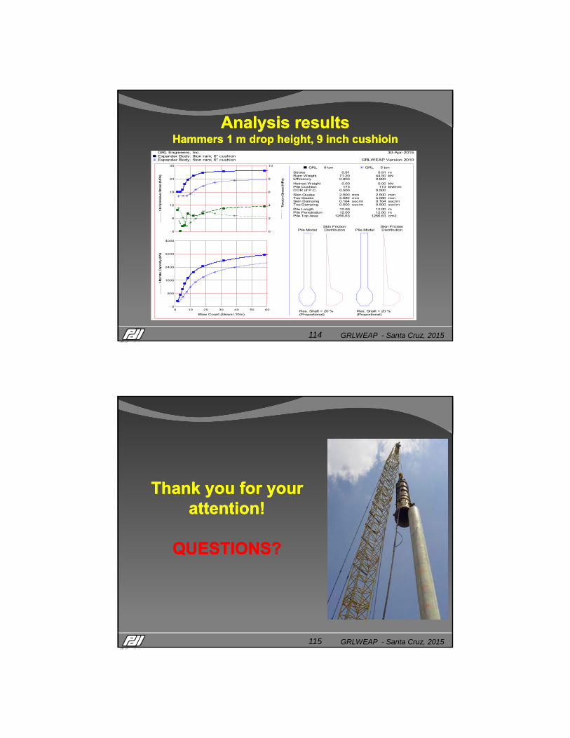
Analysis resultsHammers 1 m drop height, 9 inch cushioin

Analysis resultsHammers 1 m drop height, 9 inch cushioin

30-Apr-2015GRL Engineers, Inc. Expander Body: 8ton ram; 6" cushion

GRLWEAP Version 2010Expander Body: 5ton ram; 6" cushion

30-Apr-2015GRL Engineers, Inc. Expander Body: 8ton ram; 6" cushion

GRLWEAP Version 2010Expander Body: 5ton ram; 6" cushion Com

pre

ssive S

tress

(M

Pa)

0

6

12

18

24

30

Tension S

tress

(M

Pa)

0

2

4

6

8

10

Blow Count (blows/.10m)

Ultim

ate

Capacity (kN

)

0 10 20 30 40 50 600

800

1600

2400

3200

4000

GRL 8 ton GRL 5 ton

Stroke 0.91 0.91 mRam Weight 71.20 44.50 kNEfficiency 0.800 0.800

Helmet Weight 0.00 0.00 kNPile Cushion 173 173 kN/mmCOR of P.C. 0.500 0.500

Skin Quake 2.500 mm 2.500 mmToe Quake 5.080 mm 5.080 mmSkin Damping 0.164 sec/m 0.164 sec/mToe Damping 0.500 sec/m 0.500 sec/m

Pile LengthPile PenetrationPile Top Area

12.00 12.00

1256.63

Pile ModelSkin FrictionDistribution

Res. Shaft = 20 %(Proportional)

12.00 12.00

1256.63

m m cm2

Pile ModelSkin FrictionDistribution

Res. Shaft = 20 %(Proportional)


Thank you for your attention!

QUESTIONS?

Thank you for your attention!

QUESTIONS?