Embed Size (px)
Citation preview

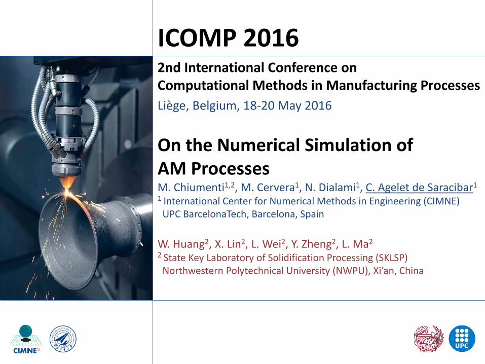
On the Numerical Simulation of AM Processes M. Chiumenti1,2, M. Cervera1, N. Dialami1, C. Agelet de Saracibar1 1 International Center for Numerical Methods in Engineering (CIMNE) UPC BarcelonaTech, Barcelona, Spain W. Huang2, X. Lin2, L. Wei2, Y. Zheng2, L. Ma2 2 State Key Laboratory of Solidification Processing (SKLSP) Northwestern Polytechnical University (NWPU), Xi’an, China
2nd International Conference on Computational Methods in Manufacturing Processes Liège, Belgium, 18-20 May 2016
ICOMP 2016
Introduction, motivation and goals Problem statement Computational model Numerical simulations Concluding remarks
Outline
Outline
June 19, 2016 Carlos Agelet de Saracibar 2

Introduction, motivation and goals o Additive Manufacturing (AM) o AM Technologies o AM Applications o Key Benefits of AM o Challenges of AM o Goals
Problem statement Computational model Numerical simulations Concluding remarks June 19, 2016 Carlos Agelet de Saracibar 3
Outline > Introduction, Motivation and Goals
Introduction, Motivation and Goals
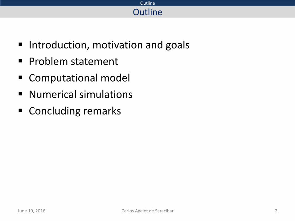
Additive Manufacturing (AM) “Additive Manufacturing (AM) is a process of joining materials to make objects from 3D model data, usually layer upon layer, as opposed to subtractive manufacturing methodologies” (ASTM-F2792-12a)
June 19, 2016 Carlos Agelet de Saracibar 4
Outline > Introduction, Motivation and Goals
Additive Manufacturing (AM)
AM Technologies
June 19, 2016 Carlos Agelet de Saracibar 5
Outline > Introduction, Motivation and Goals
AM Technologies
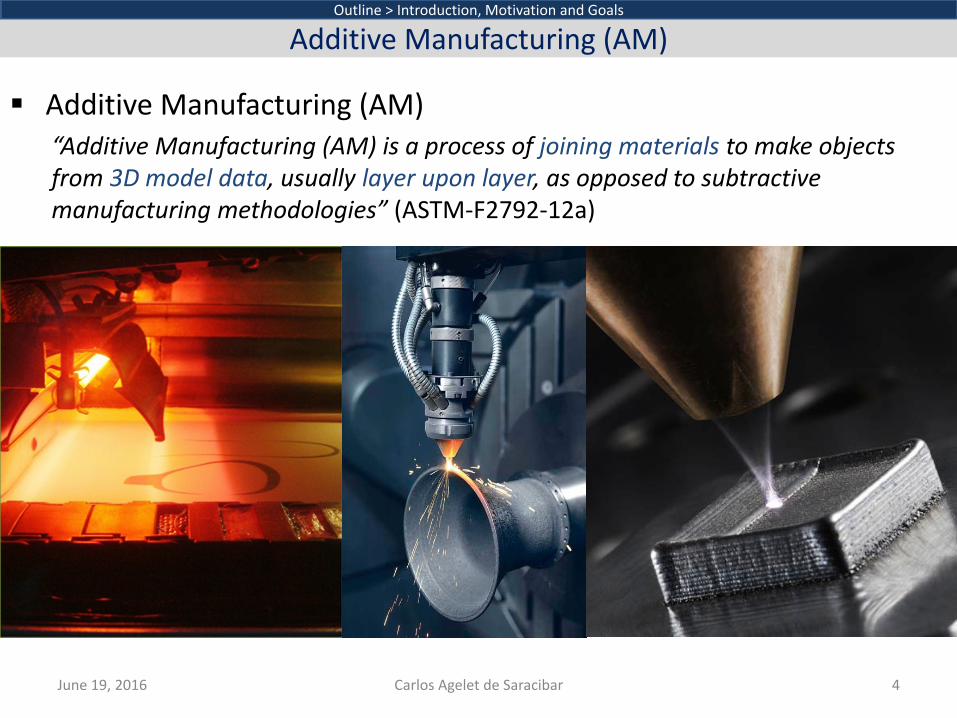
AM Powder Bed Fusion (PBF) Directed Energy Deposition (DED)
Raw material Powder Powder, Wire
Energy source Laser, EB Laser, EB, Arc welding
Deposition rate 0.1-0.2 [Kg/h] 0.5-5 [Kg/h]
Layer thickness 0.01-0.1 [mm] 0.25-3.0[mm]
Techniques Selective Laser Sintering (SLS), Selective Laser Melting (SLM), Electron Beam Melting (EBM)
Laser Metal Deposition (LMD)/Laser Engineered Net Shaping (LENS), Shaped Metal Deposition (SMD), Laser Metal Deposition-wire (LMD-w)
Features Complex Shapes, Low Deposition Rates, High Dimensional Accuracy, Small Components
Higher Deposition Rates, Lower Dimensional Accuracy, Larger Components
Applications Tooling, Functional Parts, Prototypes
Metal Part Repair, Add Features to Parts, Tooling, Functional Parts
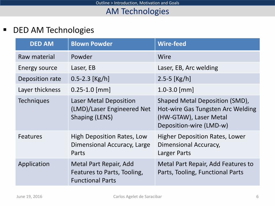
DED AM Technologies
June 19, 2016 Carlos Agelet de Saracibar 6
Outline > Introduction, Motivation and Goals
AM Technologies
DED AM Blown Powder Wire-feed
Raw material Powder Wire
Energy source Laser, EB Laser, EB, Arc welding
Deposition rate 0.5-2.3 [Kg/h] 2.5-5 [Kg/h]
Layer thickness 0.25-1.0 [mm] 1.0-3.0 [mm]
Techniques Laser Metal Deposition (LMD)/Laser Engineered Net Shaping (LENS)
Shaped Metal Deposition (SMD), Hot-wire Gas Tungsten Arc Welding (HW-GTAW), Laser Metal Deposition-wire (LMD-w)
Features High Deposition Rates, Low Dimensional Accuracy, Large Parts
Higher Deposition Rates, Lower Dimensional Accuracy, Larger Parts
Application Metal Part Repair, Add Features to Parts, Tooling, Functional Parts
Metal Part Repair, Add Features to Parts, Tooling, Functional Parts
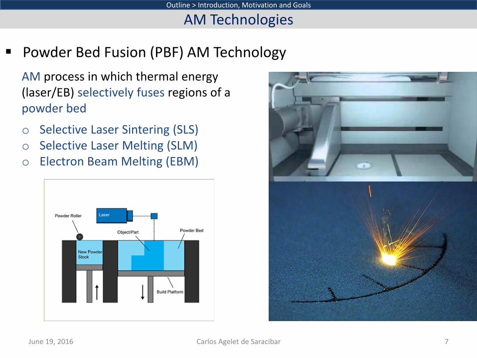
Powder Bed Fusion (PBF) AM Technology
June 19, 2016 Carlos Agelet de Saracibar 7
Outline > Introduction, Motivation and Goals
AM Technologies
AM process in which thermal energy (laser/EB) selectively fuses regions of a powder bed
o Selective Laser Sintering (SLS) o Selective Laser Melting (SLM) o Electron Beam Melting (EBM)
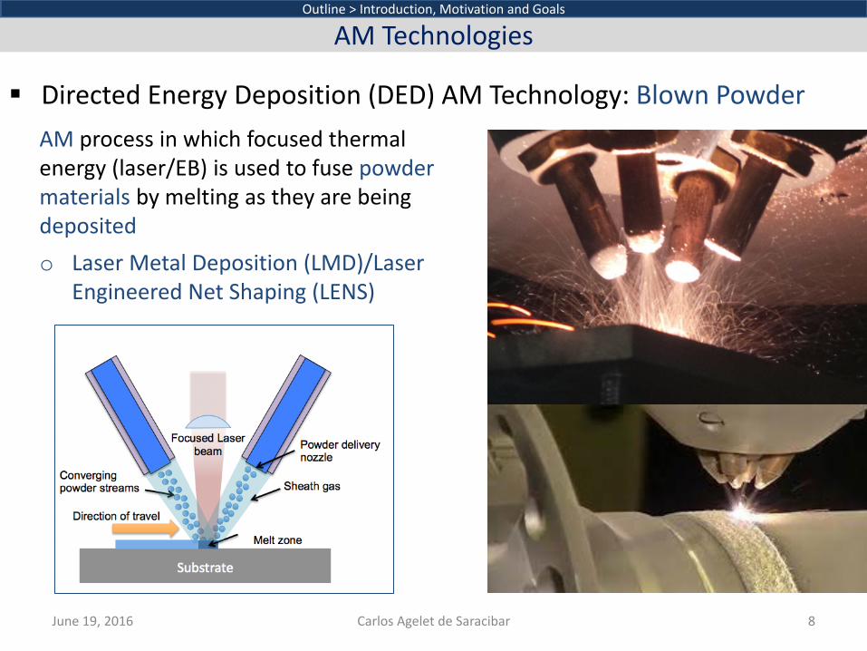
Directed Energy Deposition (DED) AM Technology: Blown Powder
June 19, 2016 Carlos Agelet de Saracibar 8
Outline > Introduction, Motivation and Goals
AM Technologies
AM process in which focused thermal energy (laser/EB) is used to fuse powder materials by melting as they are being deposited o Laser Metal Deposition (LMD)/Laser
Engineered Net Shaping (LENS)
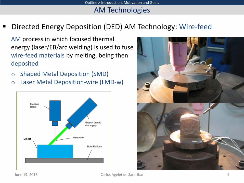
Directed Energy Deposition (DED) AM Technology: Wire-feed
June 19, 2016 Carlos Agelet de Saracibar 9
Outline > Introduction, Motivation and Goals
AM Technologies
AM process in which focused thermal energy (laser/EB/arc welding) is used to fuse wire-feed materials by melting, being then deposited o Shaped Metal Deposition (SMD) o Laser Metal Deposition-wire (LMD-w)
Object
June 19, 2016 Carlos Agelet de Saracibar 10
Outline > Introduction, Motivation and Goals
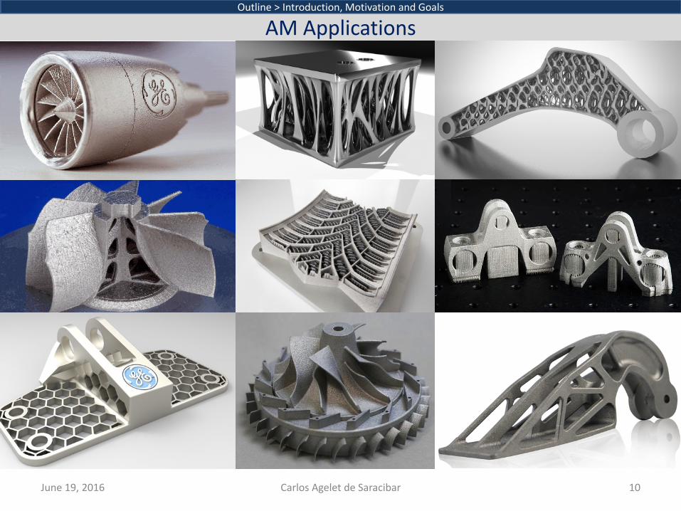
AM Applications

AM Applications: Sectors and Consumer Uses
June 19, 2016 Carlos Agelet de Saracibar 11
Outline > Introduction, Motivation and Goals
AM Applications
Source: Wohlers Report 2014 Source: Wohlers Report 2014
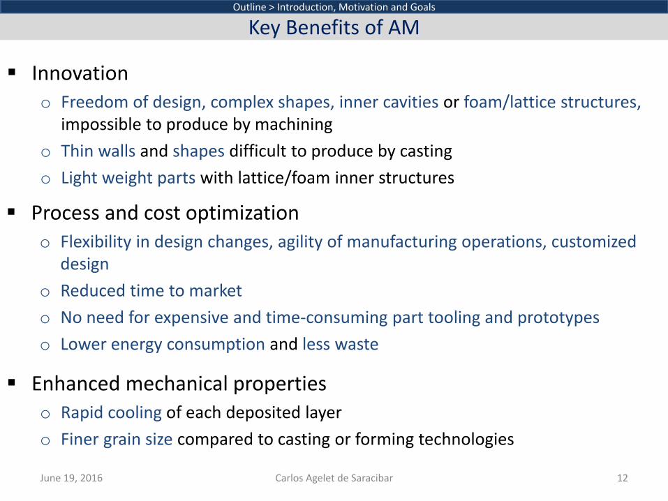
Innovation o Freedom of design, complex shapes, inner cavities or foam/lattice structures,
impossible to produce by machining o Thin walls and shapes difficult to produce by casting o Light weight parts with lattice/foam inner structures
June 19, 2016 Carlos Agelet de Saracibar 12
Outline > Introduction, Motivation and Goals
Key Benefits of AM
Process and cost optimization o Flexibility in design changes, agility of manufacturing operations, customized
design o Reduced time to market o No need for expensive and time-consuming part tooling and prototypes o Lower energy consumption and less waste
Enhanced mechanical properties
o Rapid cooling of each deposited layer o Finer grain size compared to casting or forming technologies
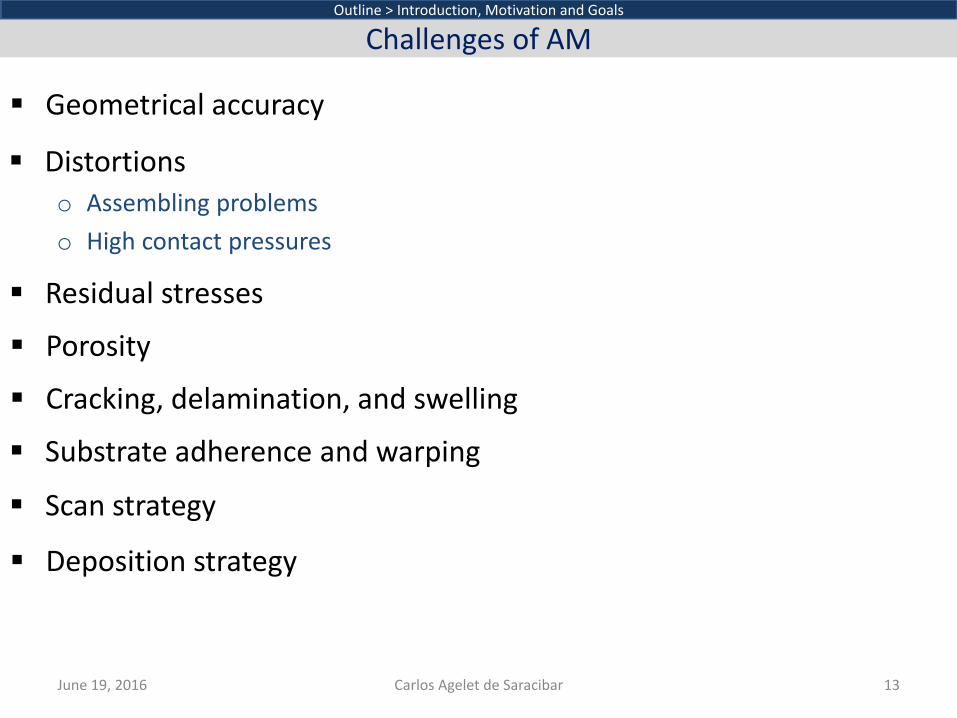
Geometrical accuracy
June 19, 2016 Carlos Agelet de Saracibar 13
Outline > Introduction, Motivation and Goals
Challenges of AM
Distortions o Assembling problems o High contact pressures
Residual stresses
Porosity
Cracking, delamination, and swelling
Substrate adherence and warping
Scan strategy
Deposition strategy
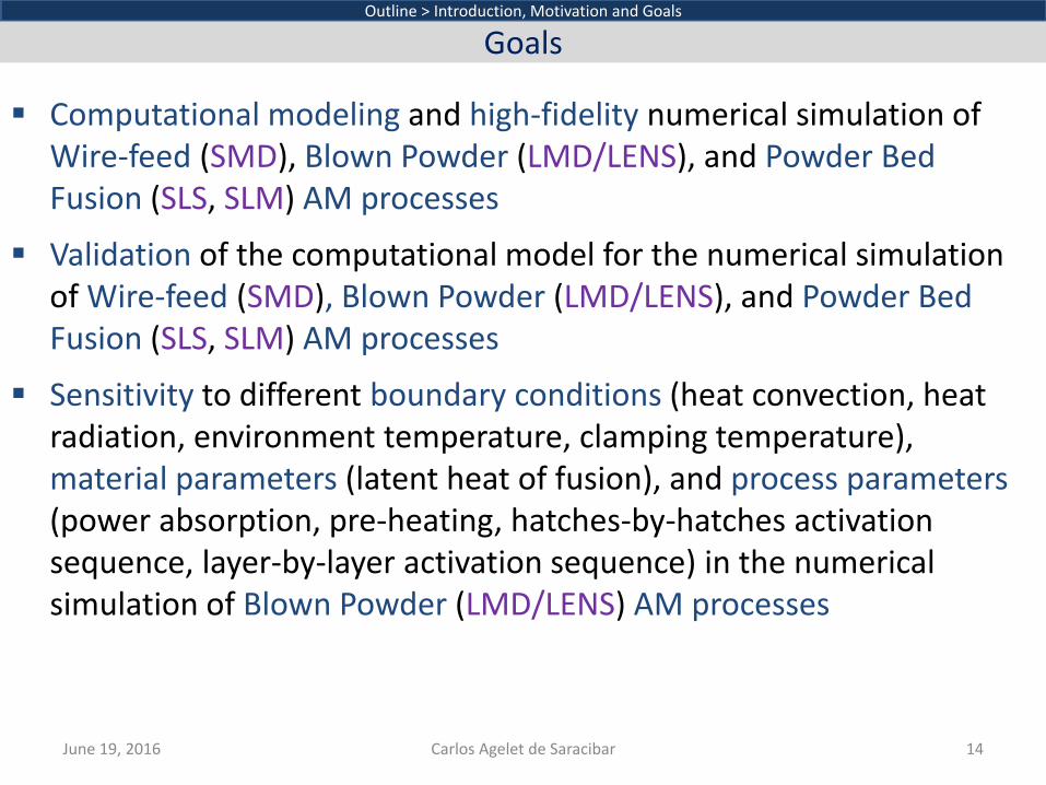
Computational modeling and high-fidelity numerical simulation of Wire-feed (SMD), Blown Powder (LMD/LENS), and Powder Bed Fusion (SLS, SLM) AM processes
June 19, 2016 Carlos Agelet de Saracibar 14
Outline > Introduction, Motivation and Goals
Goals
Validation of the computational model for the numerical simulation of Wire-feed (SMD), Blown Powder (LMD/LENS), and Powder Bed Fusion (SLS, SLM) AM processes
Sensitivity to different boundary conditions (heat convection, heat radiation, environment temperature, clamping temperature), material parameters (latent heat of fusion), and process parameters (power absorption, pre-heating, hatches-by-hatches activation sequence, layer-by-layer activation sequence) in the numerical simulation of Blown Powder (LMD/LENS) AM processes
Introduction Problem statement
o Coupled thermomechanical problem o Thermal problem o Mechanical problem
Computational model Numerical simulations Concluding remarks
Outline > Problem Statement
Problem Statement
June 19, 2016 Carlos Agelet de Saracibar 15
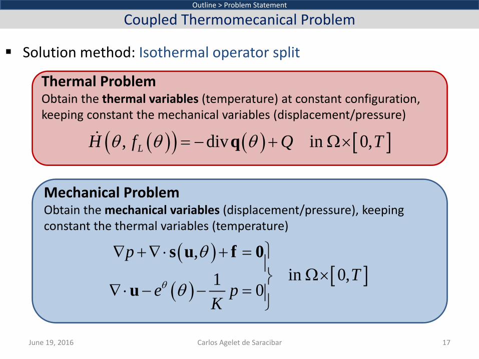
Solution method: Isothermal operator split
June 19, 2016 Carlos Agelet de Saracibar 17
Outline > Problem Statement
Coupled Thermomecanical Problem
Thermal Problem Obtain the thermal variables (temperature) at constant configuration, keeping constant the mechanical variables (displacement/pressure)
Mechanical Problem Obtain the mechanical variables (displacement/pressure), keeping constant the thermal variables (temperature)
( )( ) ( ) [ ], div in 0,LH f Q Tθ θ θ= − + Ω×q
( )
( )[ ]
,in 0,1 0
pT
e pK
θ
θ
θ
∇ +∇⋅ + = Ω×
∇⋅ − − =
s u f 0
u
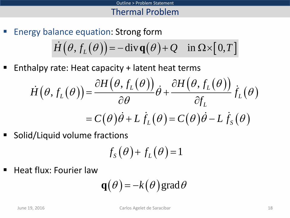
Energy balance equation: Strong form
Enthalpy rate: Heat capacity + latent heat terms
Solid/Liquid volume fractions
Heat flux: Fourier law
June 19, 2016 Carlos Agelet de Saracibar 18
Outline > Problem Statement
Thermal Problem
( )( ) ( ) [ ], div in 0,LH f Q Tθ θ θ= − + Ω×q
( )( ) ( )( ) ( )( ) ( )
( ) ( ) ( ) ( )
, ,, L L
L LL
L S
H f H fH f f
f
C L f C L f
θ θ θ θθ θ θ θ
θ
θ θ θ θ θ θ
∂ ∂= +
∂ ∂
= + = −
( ) ( )gradkθ θ θ= −q
( ) ( ) 1S Lf fθ θ+ =

Heat source: Wire-feed AM (SMD) Power input: Arc voltage: Current intensity: Power efficiency: MD volume: Wire-feed volume:
Heat source: Blown Powder (LMD/LENS)/Powder Bed Fusion AM (SLS, SLM) Laser power input: Power absorption: Melting pool volume:
June 19, 2016 Carlos Agelet de Saracibar 19
Outline > Problem Statement
Thermal Problem
eff effMD feed
P V IQV V
η η= =
effη
P
feedV
VI
absηP
poolVabs
pool
PQV
η=
MDV

Energy balance equation: Variational form
Boundary domain The boundary domain is changing during the AM process
June 19, 2016 Carlos Agelet de Saracibar 20
Outline > Problem Statement
Thermal Problem
( ) ( )( ) ( ) ( )( ) ( ) 0
, , ,
, ,clamp env
S
cond conv rad
C L f k Q
q q q
δθ θ θ θ δθ θ δθ
δθ δθ δθ∂ Ω ∂ Ω
− + ∇ ∇ =
− − + ∀ ∈
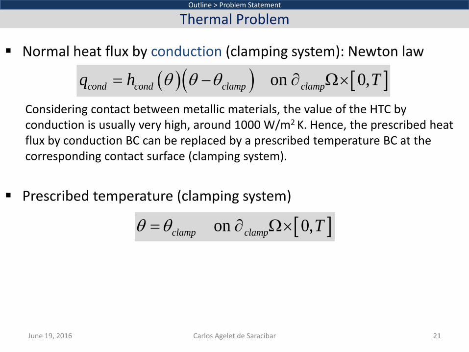
Normal heat flux by conduction (clamping system): Newton law
Considering contact between metallic materials, the value of the HTC by conduction is usually very high, around 1000 W/m2 K. Hence, the prescribed heat flux by conduction BC can be replaced by a prescribed temperature BC at the corresponding contact surface (clamping system).
Prescribed temperature (clamping system)
June 19, 2016 Carlos Agelet de Saracibar 21
Outline > Problem Statement
Thermal Problem
[ ]on 0,clamp clamp Tθ θ= ∂ Ω×
( )( ) [ ]on 0,cond cond clamp clampq h Tθ θ θ= − ∂ Ω×
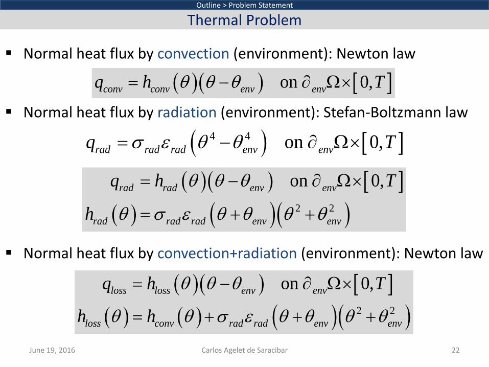
Normal heat flux by convection (environment): Newton law
Normal heat flux by radiation (environment): Stefan-Boltzmann law Normal heat flux by convection+radiation (environment): Newton law
June 19, 2016 Carlos Agelet de Saracibar 22
Outline > Problem Statement
Thermal Problem
( )( ) [ ]on 0,conv conv env envq h Tθ θ θ= − ∂ Ω×
( ) [ ]4 4 on 0,rad rad rad env envq Tσ ε θ θ= − ∂ Ω×
( )( ) [ ]( ) ( ) ( )( )2 2
on 0,loss loss env env
loss conv rad rad env env
q h T
h h
θ θ θ
θ θ σ ε θ θ θ θ
= − ∂ Ω×
= + + +
( )( ) [ ]( ) ( )( )2 2
on 0,rad rad env env
rad rad rad env env
q h T
h
θ θ θ
θ σ ε θ θ θ θ
= − ∂ Ω×
= + +
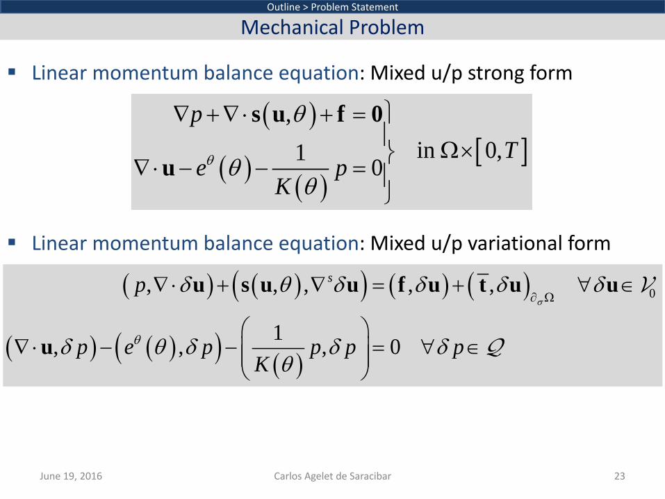
Linear momentum balance equation: Mixed u/p strong form
Linear momentum balance equation: Mixed u/p variational form
June 19, 2016 Carlos Agelet de Saracibar 23
Outline > Problem Statement
Mechanical Problem
( )
( ) ( )[ ]
,in 0,1 0
pT
e pK
θ
θ
θθ
∇ +∇⋅ + = Ω×∇⋅ − − =
s u f 0
u
( ) ( )( ) ( ) ( )
( ) ( )( ) ( )
0, , , , ,
1, , , 0
sp
p e p p p pK
σ
θ
δ θ δ δ δ δ
δ θ δ δ δθ
∂ Ω∇ ⋅ + ∇ = + ∀ ∈
∇ ⋅ − − = ∀ ∈
u s u u f u t u u
u
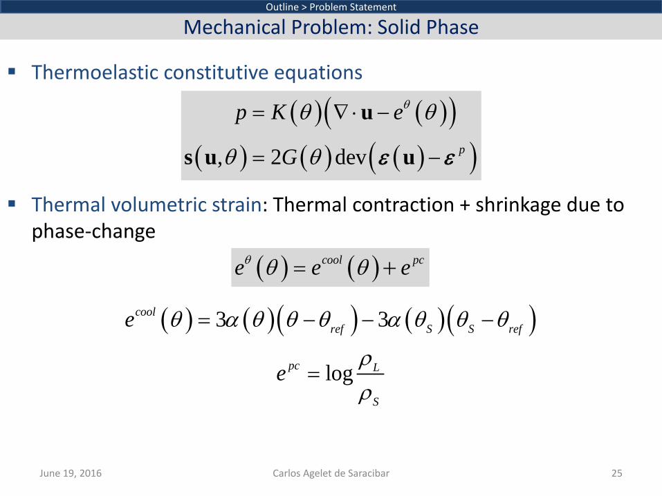
Thermoelastic constitutive equations
Thermal volumetric strain: Thermal contraction + shrinkage due to phase-change
June 19, 2016 Carlos Agelet de Saracibar 25
Outline > Problem Statement
Mechanical Problem: Solid Phase
( ) ( )( )( ) ( ) ( )( ), 2 dev p
p K e
G
θθ θ
θ θ
= ∇ ⋅ −
= −
u
s u uε ε
( ) ( )cool pce e eθ θ θ= +
logpc L
S
eρρ
=
( ) ( )( ) ( )( )3 3coolref S S refe θ α θ θ θ α θ θ θ= − − −
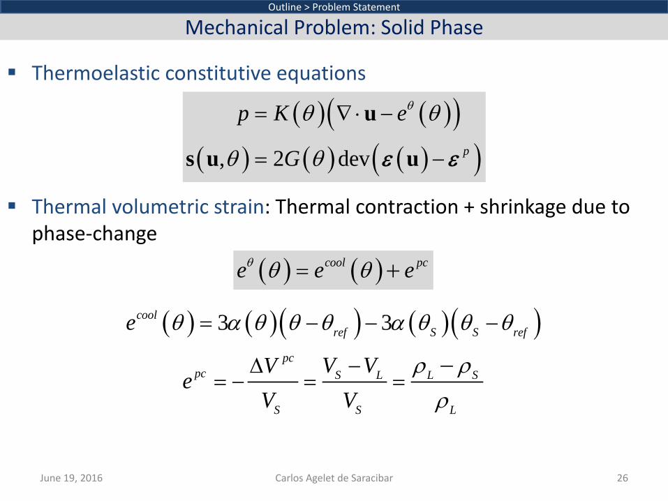
Thermoelastic constitutive equations
Thermal volumetric strain: Thermal contraction + shrinkage due to phase-change
June 19, 2016 Carlos Agelet de Saracibar 26
Outline > Problem Statement
Mechanical Problem: Solid Phase
( ) ( )( )( ) ( ) ( )( ), 2 dev p
p K e
G
θθ θ
θ θ
= ∇ ⋅ −
= −
u
s u uε ε
( ) ( )cool pce e eθ θ θ= +
pcpc S L L S
S S L
V VVe
V Vρ ρρ
−∆= − = =
−
( ) ( )( ) ( )( )3 3coolref S S refe θ α θ θ θ α θ θ θ= − − −
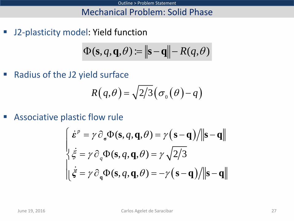
J2-plasticity model: Yield function
Radius of the J2 yield surface
Associative plastic flow rule
June 19, 2016 Carlos Agelet de Saracibar 27
Outline > Problem Statement
Mechanical Problem: Solid Phase
( , , , ) : ( , )q R qθ θΦ = − −s q s q
( ) ( )( )0, 2 3R q qθ σ θ= −
( )
( )
( , , , )
( , , , ) 2 3
( , , , )
p
q
q
q
q
γ θ γ
ξ γ θ γ
γ θ γ
= ∂ Φ = − −
= ∂ Φ =
= ∂ Φ = − − −
σ
q
s q s q s q
s q
s q s q s q
ε
ξ
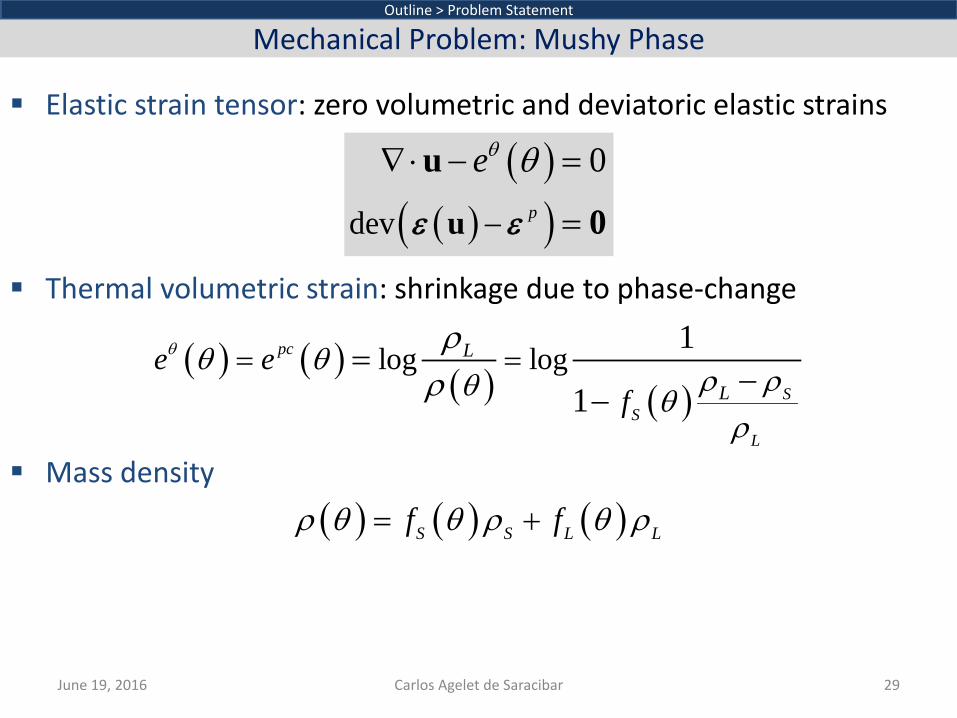
Elastic strain tensor: zero volumetric and deviatoric elastic strains Thermal volumetric strain: shrinkage due to phase-change
Mass density
June 19, 2016 Carlos Agelet de Saracibar 29
Outline > Problem Statement
Mechanical Problem: Mushy Phase
( ) ( )( ) ( )
log log1
1
pc
SS
L
L
Le e
f
θ θ θρ ρθ θρ
ρρ
= ==−
−
( ) ( ) ( )S S L Lf fρ θ θ ρ θ ρ= +
( )( )( )dev
0p
eθ θ
−
∇ ⋅ − =
=u
u
0ε ε
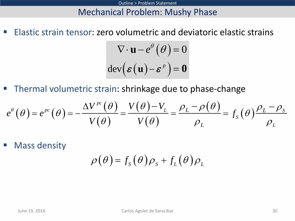
Elastic strain tensor: zero volumetric and deviatoric elastic strains Thermal volumetric strain: shrinkage due to phase-change
Mass density
June 19, 2016 Carlos Agelet de Saracibar 30
Outline > Problem Statement
Mechanical Problem: Mushy Phase
( ) ( ) ( )S S L Lf fρ θ θ ρ θ ρ= +
( ) ( ) ( )( )
( )( )
( ) ( )pc
pc L SS
L
L L
L
V V Ve e f
V Vθ θ θ ρ ρ θ ρ ρθ θ θ
θ θ ρ ρ∆
= = − = = =− − −
( )( )( )dev
0p
eθ θ
−
∇ ⋅ − =
=u
u
0ε ε
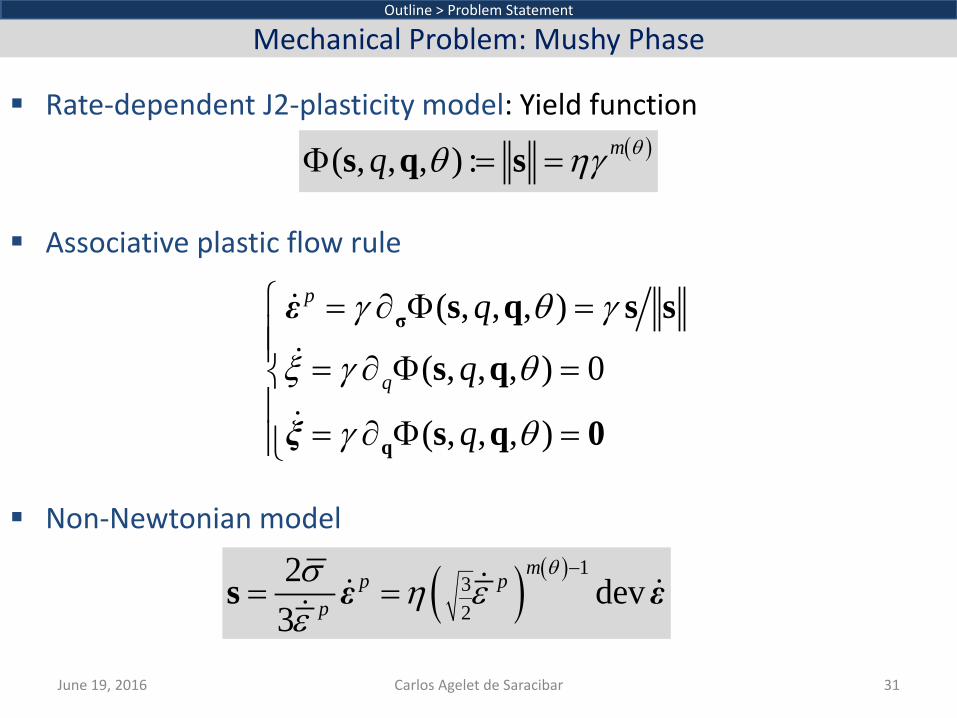
Rate-dependent J2-plasticity model: Yield function Associative plastic flow rule
Non-Newtonian model
June 19, 2016 Carlos Agelet de Saracibar 31
Outline > Problem Statement
Mechanical Problem: Mushy Phase
( )( , , , ) : mq θθ ηγΦ = =s q s
( , , , )
( , , , ) 0
( , , , )
p
q
q
q
q
γ θ γ
ξ γ θ
γ θ
= ∂ Φ = = ∂ Φ =
= ∂ Φ =
σ
q
s q s s
s q
s q 0
ε
ξ
( ) ( ) 132
2 dev3
mp p
p
θσ η εε
−= =s
ε ε
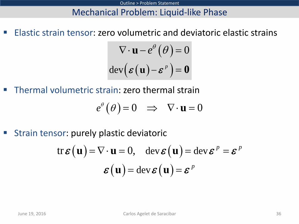
Elastic strain tensor: zero volumetric and deviatoric elastic strains Thermal volumetric strain: zero thermal strain Strain tensor: purely plastic deviatoric
June 19, 2016 Carlos Agelet de Saracibar 36
Outline > Problem Statement
Mechanical Problem: Liquid-like Phase
( )( )( )dev
0p
eθ θ
−
∇ ⋅ − =
=u
u
0ε ε
( ) 0 0eθ θ = ⇒ ∇⋅ =u
( ) ( )( ) ( )
dev dev
dev
tr 0, p p
p
= ∇⋅ = = =
= =
u u u
u u
ε ε ε ε
ε ε ε
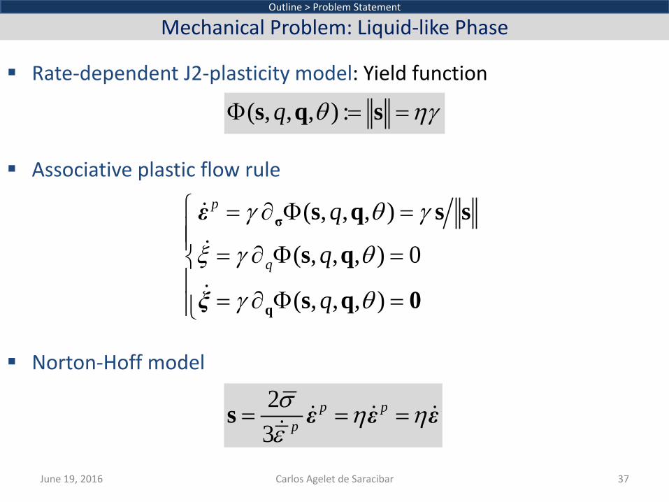
Rate-dependent J2-plasticity model: Yield function Associative plastic flow rule
Norton-Hoff model
June 19, 2016 Carlos Agelet de Saracibar 37
Outline > Problem Statement
Mechanical Problem: Liquid-like Phase
( , , , ) :q θ ηγΦ = =s q s
( , , , )
( , , , ) 0
( , , , )
p
q
q
q
q
γ θ γ
ξ γ θ
γ θ
= ∂ Φ = = ∂ Φ =
= ∂ Φ =
σ
q
s q s s
s q
s q 0
ε
ξ
23
p pp
σ η ηε
= = =s
ε ε ε

Introduction Problem statement Computational model
o FE Activation strategy o Welding pool volume o Scanning path: Common Layer Interface (CLI) o Incompressibility constraint
Numerical simulations Concluding remarks
Outline > Computational Model
Computational Model
June 19, 2016 Carlos Agelet de Saracibar 45
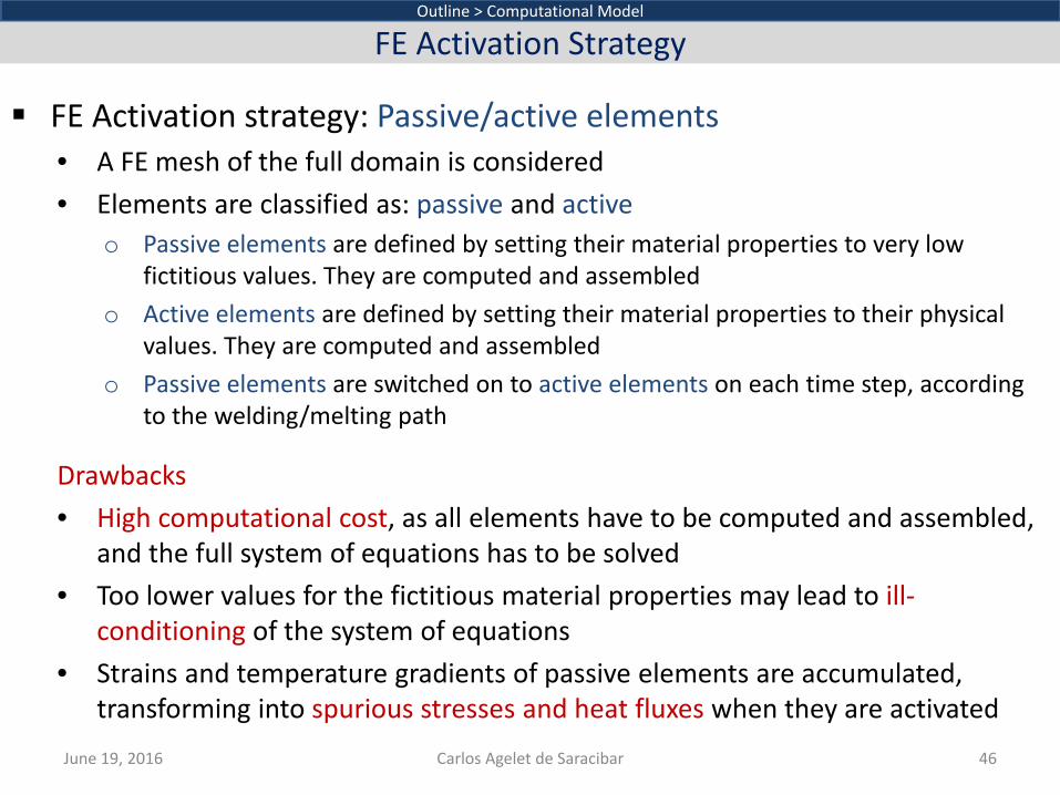
FE Activation strategy: Passive/active elements • A FE mesh of the full domain is considered • Elements are classified as: passive and active
o Passive elements are defined by setting their material properties to very low fictitious values. They are computed and assembled
o Active elements are defined by setting their material properties to their physical values. They are computed and assembled
o Passive elements are switched on to active elements on each time step, according to the welding/melting path
June 19, 2016 Carlos Agelet de Saracibar 46
Outline > Computational Model
FE Activation Strategy
Drawbacks • High computational cost, as all elements have to be computed and assembled,
and the full system of equations has to be solved • Too lower values for the fictitious material properties may lead to ill-
conditioning of the system of equations • Strains and temperature gradients of passive elements are accumulated,
transforming into spurious stresses and heat fluxes when they are activated
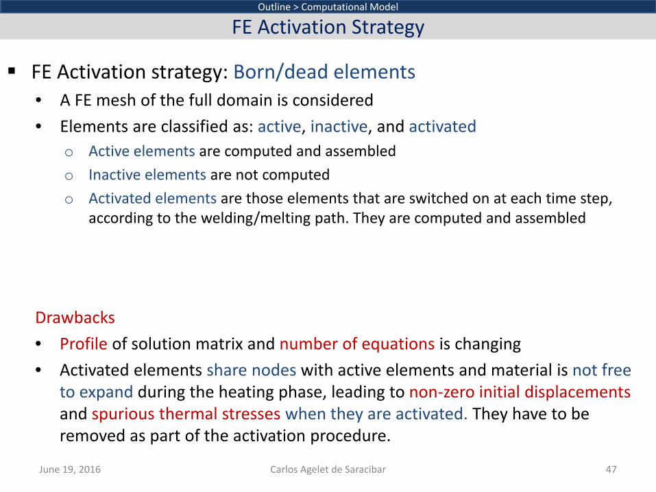
FE Activation strategy: Born/dead elements • A FE mesh of the full domain is considered • Elements are classified as: active, inactive, and activated
o Active elements are computed and assembled o Inactive elements are not computed o Activated elements are those elements that are switched on at each time step,
according to the welding/melting path. They are computed and assembled
June 19, 2016 Carlos Agelet de Saracibar 47
Outline > Computational Model
FE Activation Strategy
Drawbacks • Profile of solution matrix and number of equations is changing • Activated elements share nodes with active elements and material is not free
to expand during the heating phase, leading to non-zero initial displacements and spurious thermal stresses when they are activated. They have to be removed as part of the activation procedure.
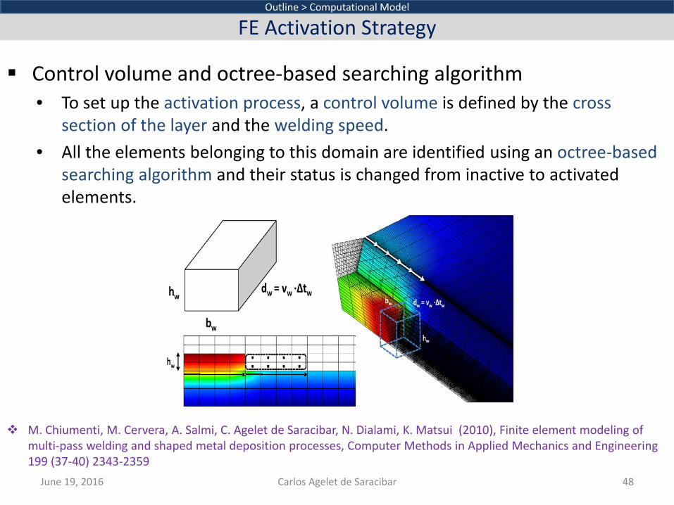
Control volume and octree-based searching algorithm • To set up the activation process, a control volume is defined by the cross
section of the layer and the welding speed. • All the elements belonging to this domain are identified using an octree-based
searching algorithm and their status is changed from inactive to activated elements.
June 19, 2016 Carlos Agelet de Saracibar 48
Outline > Computational Model
FE Activation Strategy
M. Chiumenti, M. Cervera, A. Salmi, C. Agelet de Saracibar, N. Dialami, K. Matsui (2010), Finite element modeling of multi-pass welding and shaped metal deposition processes, Computer Methods in Applied Mechanics and Engineering 199 (37-40) 2343-2359
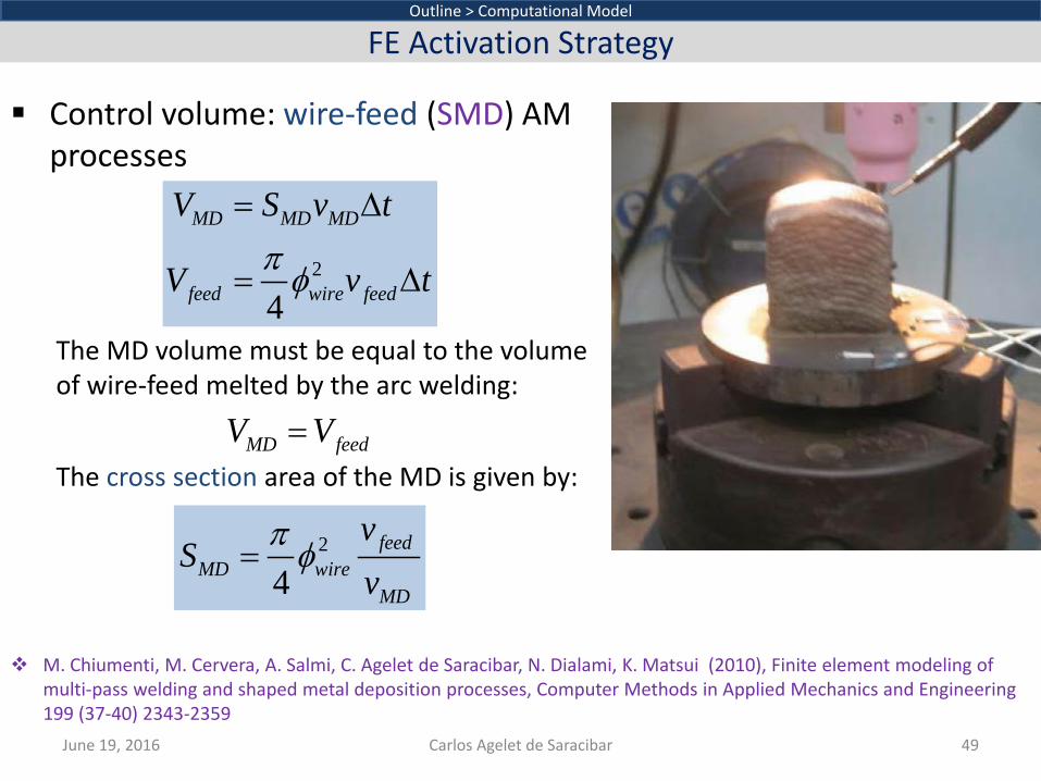
Control volume: wire-feed (SMD) AM processes
The MD volume must be equal to the volume of wire-feed melted by the arc welding:
The cross section area of the MD is given by:
June 19, 2016 Carlos Agelet de Saracibar 49
Outline > Computational Model
FE Activation Strategy
MD feedV V=
2
4
MD MD MD
feed wire feed
V S v t
V v tπ φ
= ∆
= ∆
2
4feed
MD wireMD
vS
vπ φ=
M. Chiumenti, M. Cervera, A. Salmi, C. Agelet de Saracibar, N. Dialami, K. Matsui (2010), Finite element modeling of multi-pass welding and shaped metal deposition processes, Computer Methods in Applied Mechanics and Engineering 199 (37-40) 2343-2359
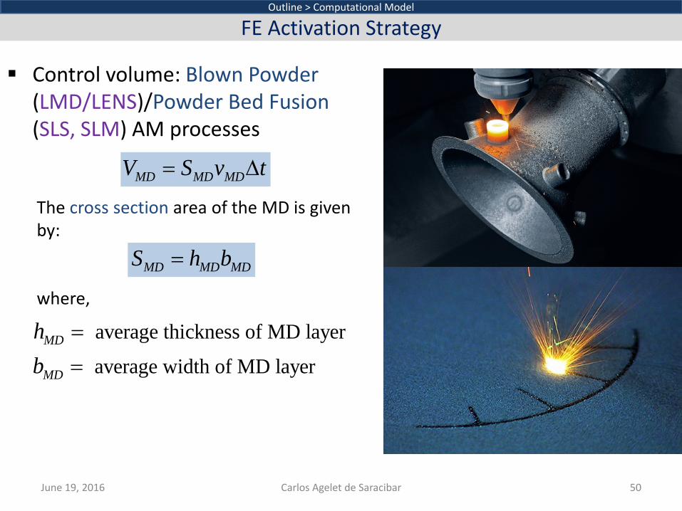
Control volume: Blown Powder (LMD/LENS)/Powder Bed Fusion (SLS, SLM) AM processes
The cross section area of the MD is given by:
where,
June 19, 2016 Carlos Agelet de Saracibar 50
Outline > Computational Model
FE Activation Strategy
MD MD MDS h b=
MD MD MDV S v t= ∆
average thickness of MD layer
average width of MD layer
MD
MD
hb
==
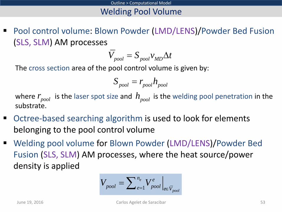
Pool control volume: Blown Powder (LMD/LENS)/Powder Bed Fusion (SLS, SLM) AM processes The cross section area of the pool control volume is given by:
where is the laser spot size and is the welding pool penetration in the substrate.
Octree-based searching algorithm is used to look for elements belonging to the pool control volume
Welding pool volume for Blown Powder (LMD/LENS)/Powder Bed Fusion (SLS, SLM) AM processes, where the heat source/power density is applied
June 19, 2016 Carlos Agelet de Saracibar 53
Outline > Computational Model
Welding Pool Volume
pool pool poolS r h=
pool pool MDV S v t= ∆
poolh
1e
pool
n epool poole e V
V V= ∈
=∑
poolr

The Common Layer Interface (CLI) is a universal format for the input of geometry data to model fabrication systems based on layer manufacturing technologies (LMT), such as LMD/LENS, SLS, or SLM
Definition of the scanning sequence using the CLI format o Layer defines the layer entry level o Polyline defines the section boundaries of the layer o Hatches define the filling section of the layer
June 19, 2016 Carlos Agelet de Saracibar 54
Outline > Computational Model
Scanning Path: Common Layer Interface (CLI)
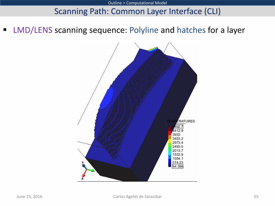
LMD/LENS scanning sequence: Polyline and hatches for a layer
June 19, 2016 Carlos Agelet de Saracibar 55
Outline > Computational Model
Scanning Path: Common Layer Interface (CLI)
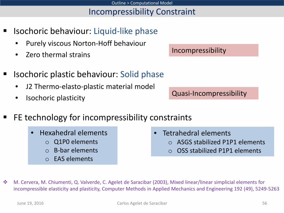
Isochoric behaviour: Liquid-like phase • Purely viscous Norton-Hoff behaviour • Zero thermal strains
Isochoric plastic behaviour: Solid phase • J2 Thermo-elasto-plastic material model • Isochoric plasticity
FE technology for incompressibility constraints M. Cervera, M. Chiumenti, Q. Valverde, C. Agelet de Saracibar (2003), Mixed linear/linear simplicial elements for
incompressible elasticity and plasticity, Computer Methods in Applied Mechanics and Engineering 192 (49), 5249-5263
June 19, 2016 Carlos Agelet de Saracibar 56
Outline > Computational Model
Incompressibility Constraint
• Hexahedral elements o Q1P0 elements o B-bar elements o EAS elements
• Tetrahedral elements o ASGS stabilized P1P1 elements o OSS stabilized P1P1 elements
Incompressibility
Quasi-Incompressibility
Introduction Problem statement Computational model Numerical simulations
o SMD Boss o SMD 10 Layers Strip Band o SMD Hanging Lug of a Jet Engine Turbine Blade o LMD/LENS 10 Layers Strip Band
Concluding remarks
Outline > Numerical Simulations
Numerical Simulations
June 19, 2016 Carlos Agelet de Saracibar 59
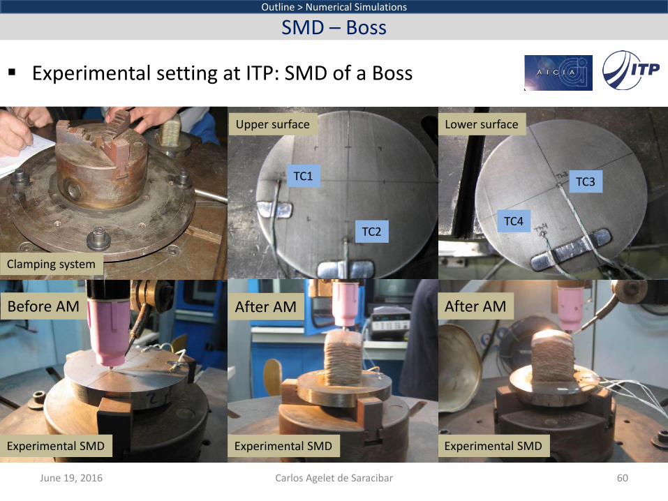
Experimental setting at ITP: SMD of a Boss
June 19, 2016 Carlos Agelet de Saracibar 60
Outline > Numerical Simulations
SMD – Boss
TC1
TC2
Upper surface Lower surface
TC3
TC4
Clamping system
Experimental SMD Experimental SMD Experimental SMD
Before AM After AM After AM
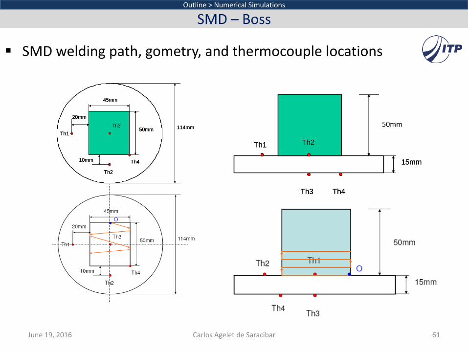
SMD welding path, gometry, and thermocouple locations
June 19, 2016 Carlos Agelet de Saracibar 61
Outline > Numerical Simulations
SMD – Boss
114mm
45mm
50mm
10mm
20mm
Th2
Th4
Th1Th3 114mm
45mm
50mm
10mm
20mm
Th2
Th4
Th1Th3
Th3 Th4
Th2Th1
45mm
15mm
Th3 Th4
Th2Th1
45mm
15mm
50mm
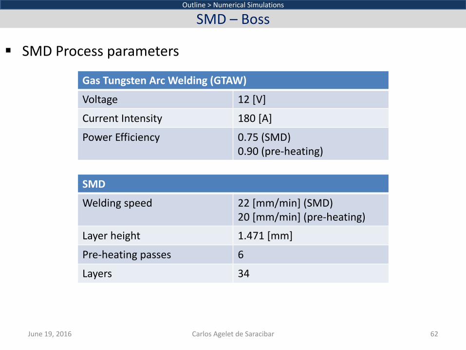
SMD Process parameters
June 19, 2016 Carlos Agelet de Saracibar 62
Outline > Numerical Simulations
SMD – Boss
Gas Tungsten Arc Welding (GTAW)
Voltage 12 [V]
Current Intensity 180 [A]
Power Efficiency 0.75 (SMD) 0.90 (pre-heating)
SMD
Welding speed 22 [mm/min] (SMD) 20 [mm/min] (pre-heating)
Layer height 1.471 [mm]
Pre-heating passes 6
Layers 34

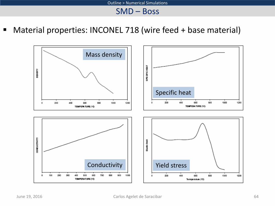
Material properties: INCONEL 718 (wire feed + base material)
June 19, 2016 Carlos Agelet de Saracibar 63
Outline > Numerical Simulations
SMD – Boss
INCONEL 718
Solidus Temperature 1260 [ºC]
Liquidus Temperature 1335 [ºC]
Latent Heat 240 [kJ/kg]
Thermal Shrinkage 3 %
Mass Density Temperature dependent
Specific Heat Temperature dependent
Thermal Conductivity Temperature dependent
Yield Stress Temperature dependent
Material properties: INCONEL 718 (wire feed + base material)
June 19, 2016 Carlos Agelet de Saracibar 64
Outline > Numerical Simulations
SMD – Boss
Mass density
Conductivity
Specific heat
Yield stress
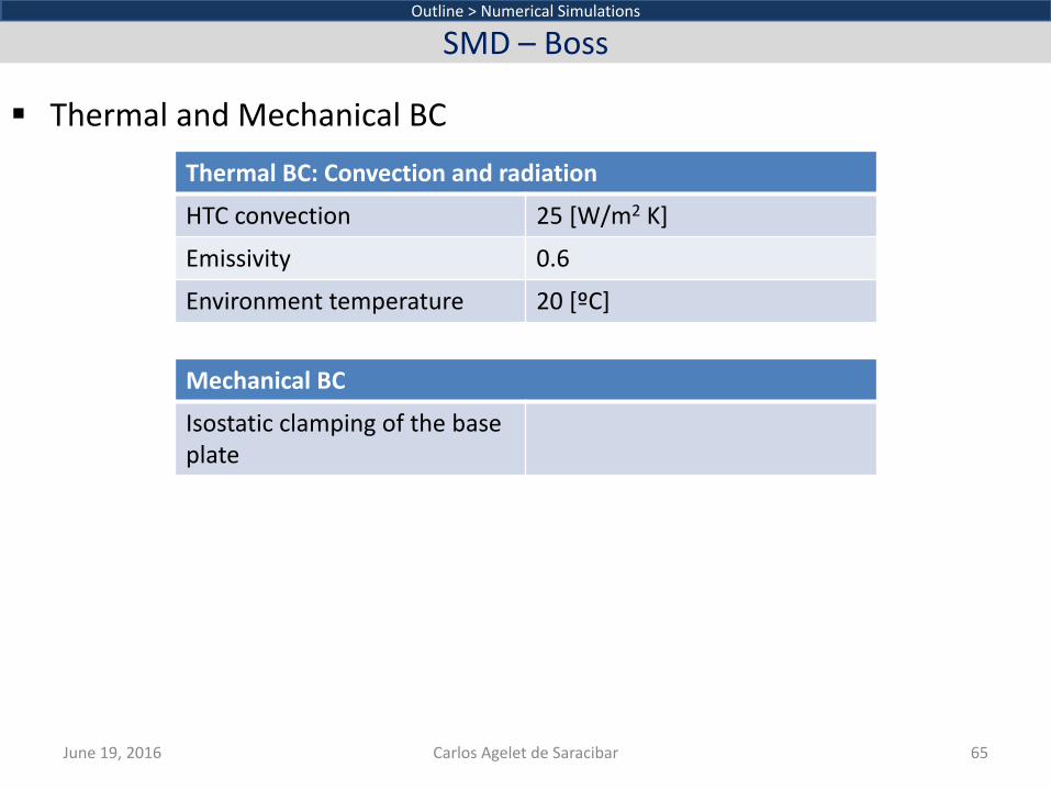
Thermal and Mechanical BC
June 19, 2016 Carlos Agelet de Saracibar 65
Outline > Numerical Simulations
SMD – Boss
Thermal BC: Convection and radiation
HTC convection 25 [W/m2 K]
Emissivity 0.6
Environment temperature 20 [ºC]
Mechanical BC
Isostatic clamping of the base plate
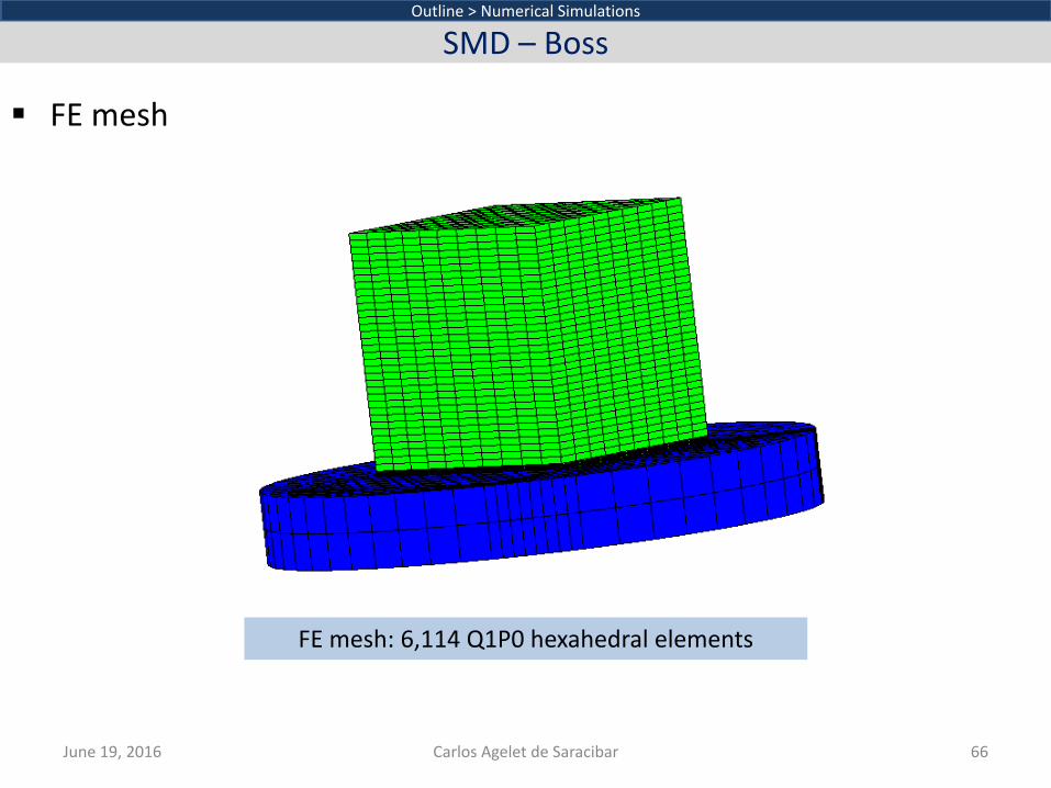
FE mesh
June 19, 2016 Carlos Agelet de Saracibar 66
Outline > Numerical Simulations
SMD – Boss
FE mesh: 6,114 Q1P0 hexahedral elements
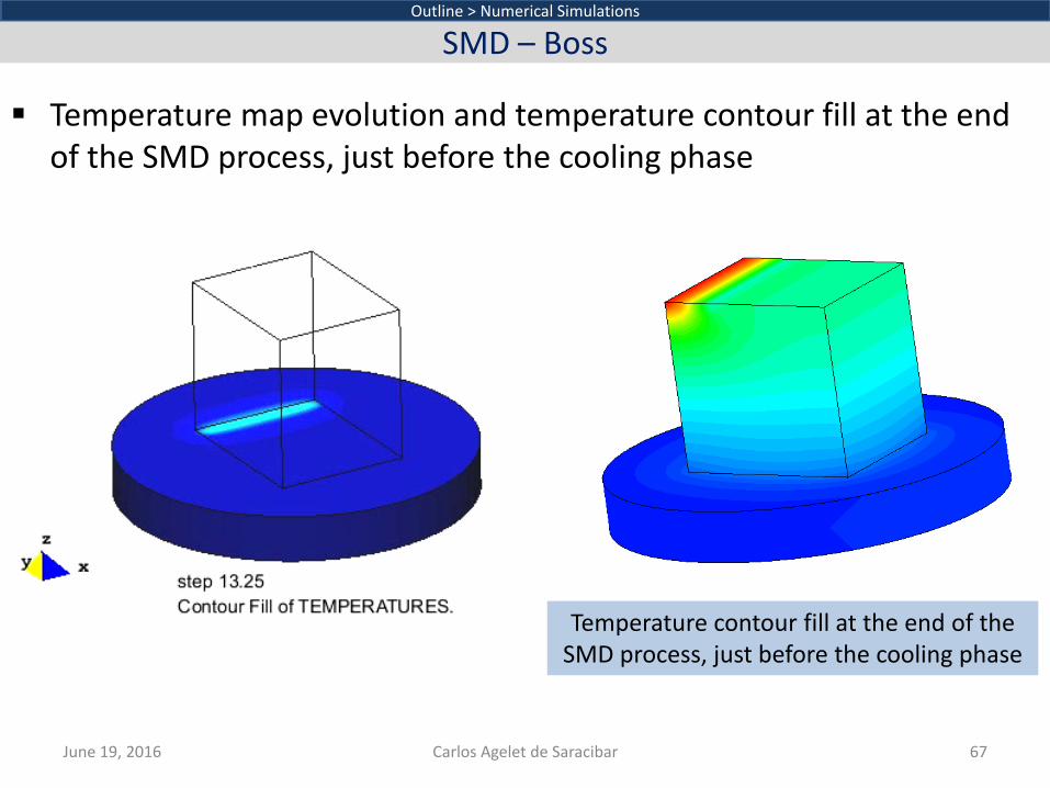
Temperature map evolution and temperature contour fill at the end of the SMD process, just before the cooling phase
June 19, 2016 Carlos Agelet de Saracibar 67
Outline > Numerical Simulations
SMD – Boss
Temperature contour fill at the end of the SMD process, just before the cooling phase
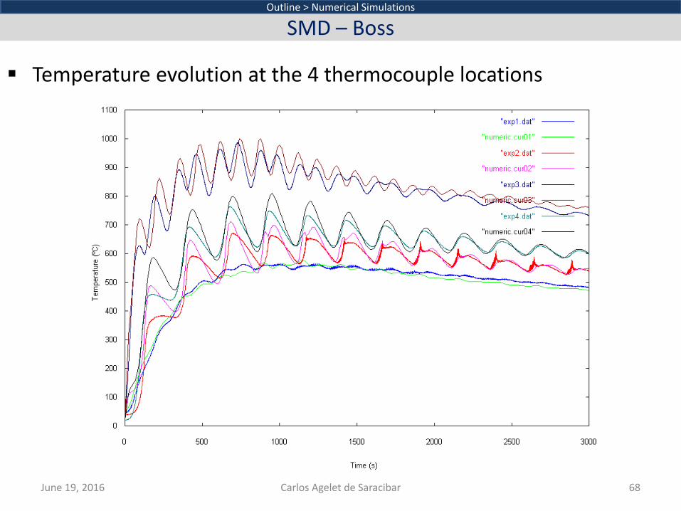
Temperature evolution at the 4 thermocouple locations
June 19, 2016 Carlos Agelet de Saracibar 68
Outline > Numerical Simulations
SMD – Boss
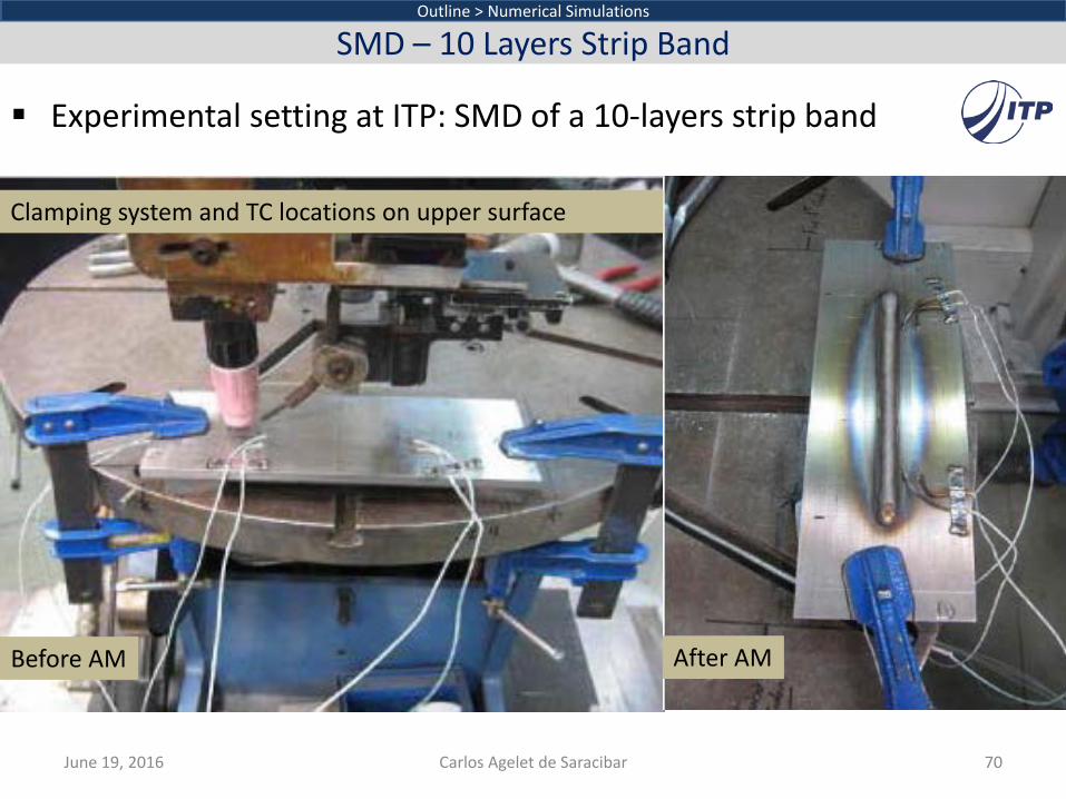
Experimental setting at ITP: SMD of a 10-layers strip band
June 19, 2016 Carlos Agelet de Saracibar 70
Outline > Numerical Simulations
SMD – 10 Layers Strip Band
Before AM After AM
Clamping system and TC locations on upper surface
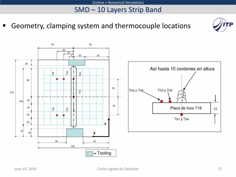
Geometry, clamping system and thermocouple locations
June 19, 2016 Carlos Agelet de Saracibar 71
Outline > Numerical Simulations
SMD – 10 Layers Strip Band

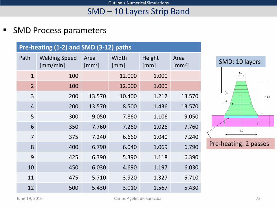
SMD Process parameters
June 19, 2016 Carlos Agelet de Saracibar 72
Outline > Numerical Simulations
SMD – 10 Layers Strip Band
Gas Tungsten Arc Welding (GTAW)
Voltage 12 [V]
Current Intensity 180 [A]
Power Efficiency 0.75 (SMD) 0.90 (pre-heating)
SMD
Welding speed Variable
Layer height Variable
Pre-heating passes 2
Layers 10
SMD Process parameters
June 19, 2016 Carlos Agelet de Saracibar 73
Outline > Numerical Simulations
SMD – 10 Layers Strip Band
Pre-heating (1-2) and SMD (3-12) paths Path Welding Speed
[mm/min] Area [mm2]
Width [mm]
Height [mm]
Area [mm2]
1 100 12.000 1.000
2 100 12.000 1.000
3 200 13.570 10.400 1.212 13.570
4 200 13.570 8.500 1.436 13.570
5 300 9.050 7.860 1.106 9.050
6 350 7.760 7.260 1.026 7.760
7 375 7.240 6.660 1.040 7.240
8 400 6.790 6.040 1.069 6.790
9 425 6.390 5.390 1.118 6.390
10 450 6.030 4.690 1.197 6.030
11 475 5.710 3.920 1.327 5.710
12 500 5.430 3.010 1.567 5.430
SMD: 10 layers
Pre-heating: 2 passes
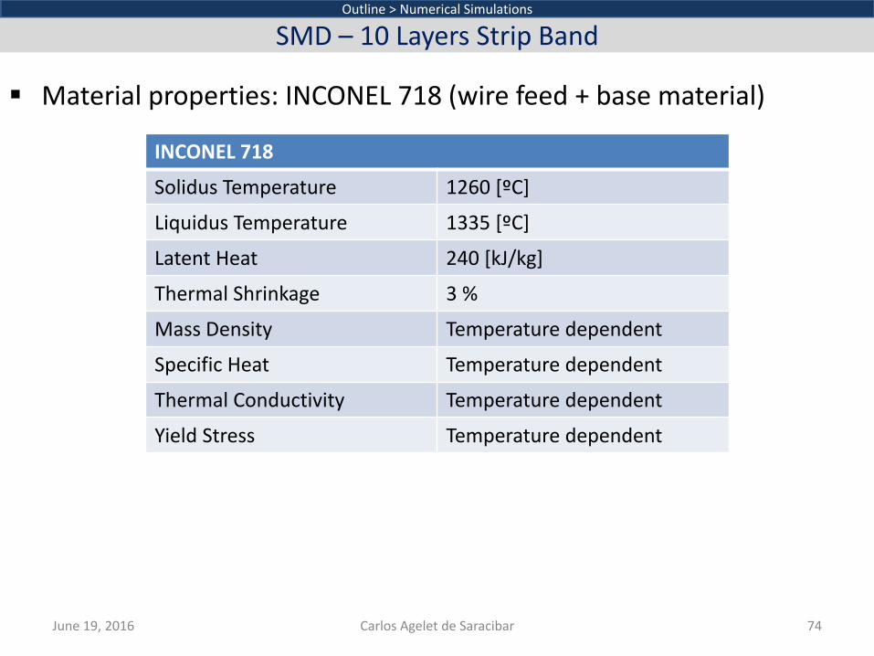
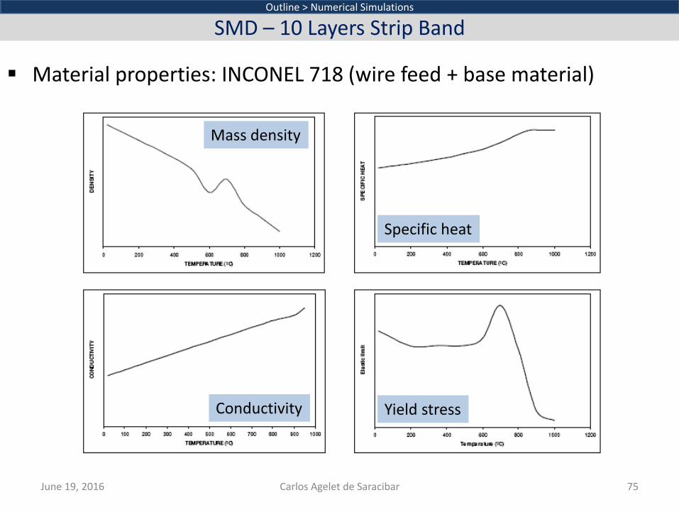
Material properties: INCONEL 718 (wire feed + base material)
June 19, 2016 Carlos Agelet de Saracibar 74
Outline > Numerical Simulations
SMD – 10 Layers Strip Band
INCONEL 718
Solidus Temperature 1260 [ºC]
Liquidus Temperature 1335 [ºC]
Latent Heat 240 [kJ/kg]
Thermal Shrinkage 3 %
Mass Density Temperature dependent
Specific Heat Temperature dependent
Thermal Conductivity Temperature dependent
Yield Stress Temperature dependent
Material properties: INCONEL 718 (wire feed + base material)
June 19, 2016 Carlos Agelet de Saracibar 75
Outline > Numerical Simulations
SMD – 10 Layers Strip Band
Mass density
Conductivity
Specific heat
Yield stress
Thermal and Mechanical BC
June 19, 2016 Carlos Agelet de Saracibar 76
Outline > Numerical Simulations
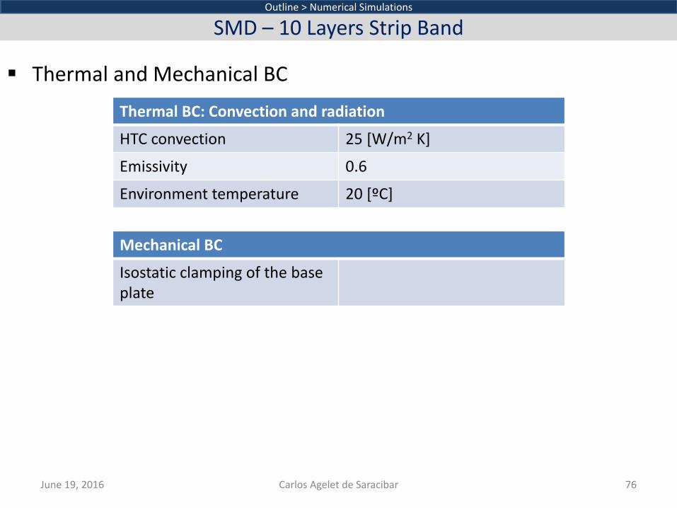
SMD – 10 Layers Strip Band
Thermal BC: Convection and radiation
HTC convection 25 [W/m2 K]
Emissivity 0.6
Environment temperature 20 [ºC]
Mechanical BC
Isostatic clamping of the base plate
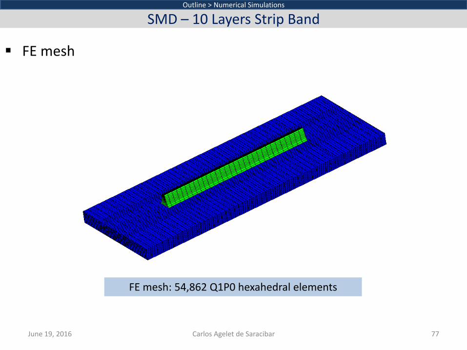
FE mesh
June 19, 2016 Carlos Agelet de Saracibar 77
Outline > Numerical Simulations
SMD – 10 Layers Strip Band
FE mesh: 54,862 Q1P0 hexahedral elements
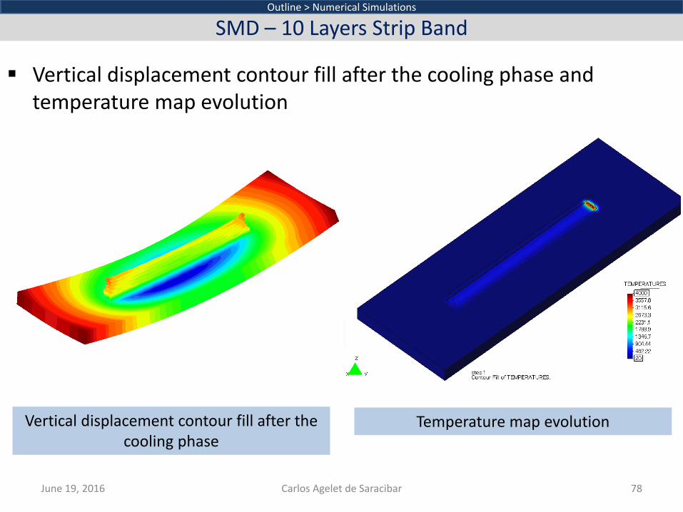
Vertical displacement contour fill after the cooling phase and temperature map evolution
June 19, 2016 Carlos Agelet de Saracibar 78
Outline > Numerical Simulations
SMD – 10 Layers Strip Band
Vertical displacement contour fill after the cooling phase
Temperature map evolution

Temperature evolution at the 6 thermocouple locations
June 19, 2016 Carlos Agelet de Saracibar 79
Outline > Numerical Simulations
SMD – 10 Layers Strip Band
0
100
200
300
400
500
600
700
800
900
0 50 100 150 200 250 300 350 400 450 500
Time (sec)
Tem
p.
Point1 Exp.
Point1 Num.
Point4 Exp.
Point4 Num.
0
100
200
300
400
500
600
700
800
900
0 50 100 150 200 250 300 350 400 450 500
Time (sec)
Tem
p
Point3 Exp.
Point3 Num.
Point5 Exp.
Point5 Num.
0
100
200
300
400
500
600
700
0 50 100 150 200 250 300 350 400 450 500
Time (sec)
Tem
p.
Point2 Exp.
Point2 Num.
Point6 Exp.
Point6 Num.
Lower surface: TC1 and TC4
Upper surface: TC2 and TC6 Upper surface: TC3 and TC5
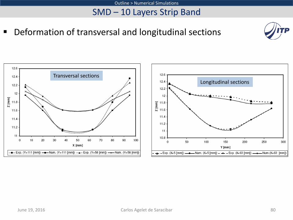
Deformation of transversal and longitudinal sections
June 19, 2016 Carlos Agelet de Saracibar 80
Outline > Numerical Simulations
SMD – 10 Layers Strip Band
Transversal sections Longitudinal sections
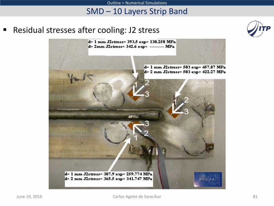
Residual stresses after cooling: J2 stress
June 19, 2016 Carlos Agelet de Saracibar 81
Outline > Numerical Simulations
SMD – 10 Layers Strip Band
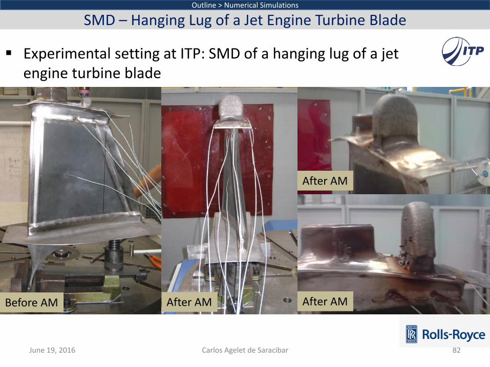
Experimental setting at ITP: SMD of a hanging lug of a jet engine turbine blade
June 19, 2016 Carlos Agelet de Saracibar 82
Outline > Numerical Simulations
SMD – Hanging Lug of a Jet Engine Turbine Blade
Before AM After AM After AM
After AM
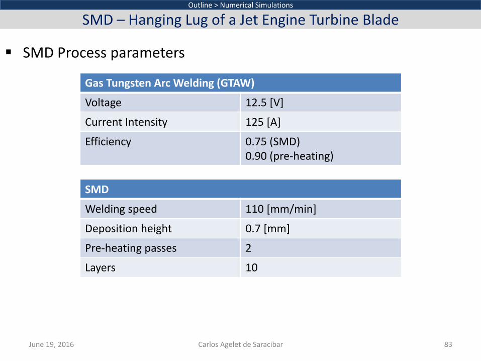
SMD Process parameters
June 19, 2016 Carlos Agelet de Saracibar 83
Outline > Numerical Simulations
SMD – Hanging Lug of a Jet Engine Turbine Blade
Gas Tungsten Arc Welding (GTAW)
Voltage 12.5 [V]
Current Intensity 125 [A]
Efficiency 0.75 (SMD) 0.90 (pre-heating)
SMD
Welding speed 110 [mm/min]
Deposition height 0.7 [mm]
Pre-heating passes 2
Layers 10
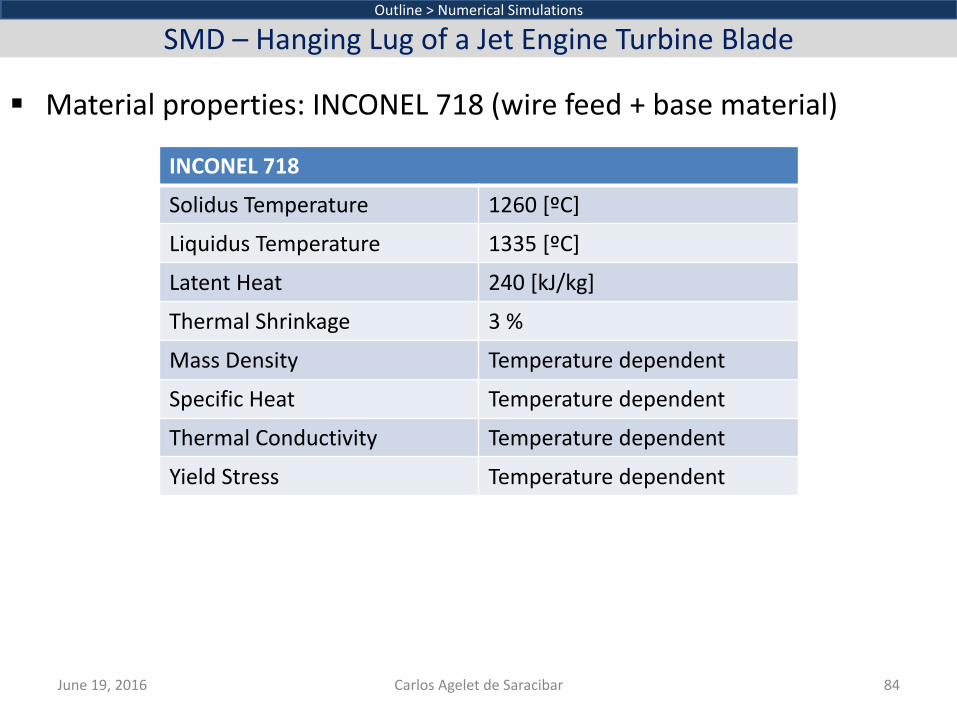
Material properties: INCONEL 718 (wire feed + base material)
June 19, 2016 Carlos Agelet de Saracibar 84
Outline > Numerical Simulations
SMD – Hanging Lug of a Jet Engine Turbine Blade
INCONEL 718
Solidus Temperature 1260 [ºC]
Liquidus Temperature 1335 [ºC]
Latent Heat 240 [kJ/kg]
Thermal Shrinkage 3 %
Mass Density Temperature dependent
Specific Heat Temperature dependent
Thermal Conductivity Temperature dependent
Yield Stress Temperature dependent
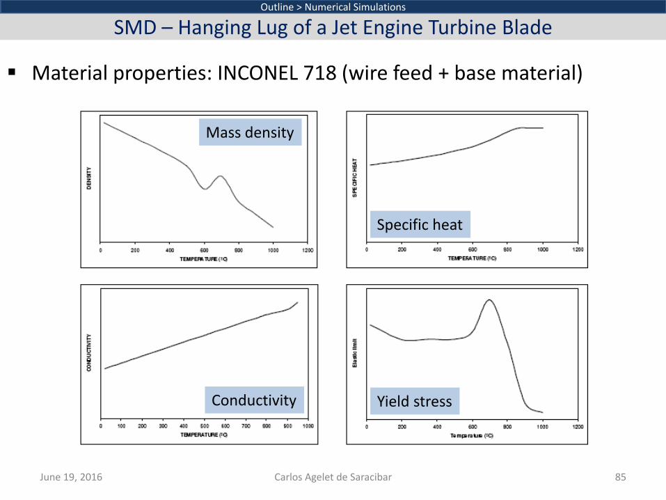
Material properties: INCONEL 718 (wire feed + base material)
June 19, 2016 Carlos Agelet de Saracibar 85
Outline > Numerical Simulations
SMD – Hanging Lug of a Jet Engine Turbine Blade
Mass density
Conductivity
Specific heat
Yield stress
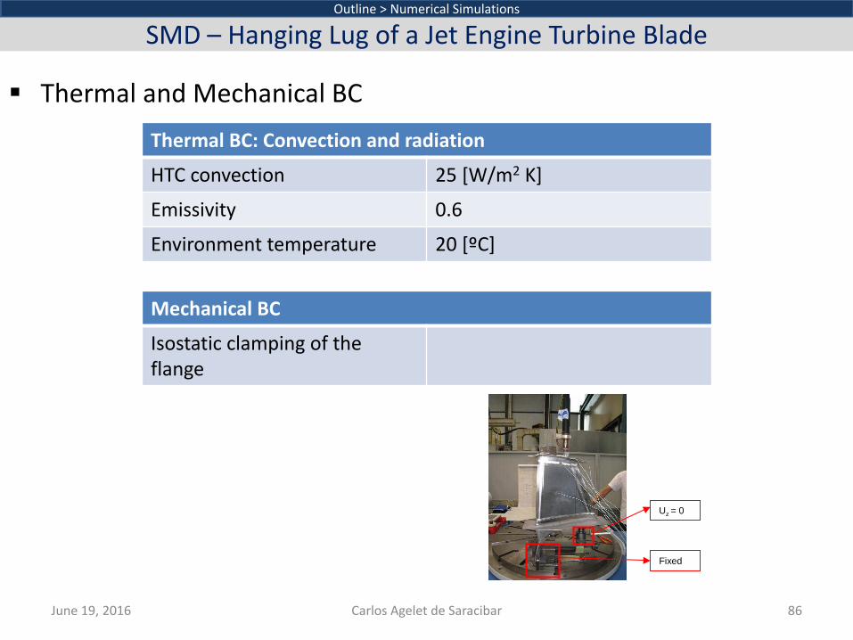
Thermal and Mechanical BC
June 19, 2016 Carlos Agelet de Saracibar 86
Outline > Numerical Simulations
SMD – Hanging Lug of a Jet Engine Turbine Blade
Thermal BC: Convection and radiation
HTC convection 25 [W/m2 K]
Emissivity 0.6
Environment temperature 20 [ºC]
Mechanical BC
Isostatic clamping of the flange
Fixed
Uz = 0
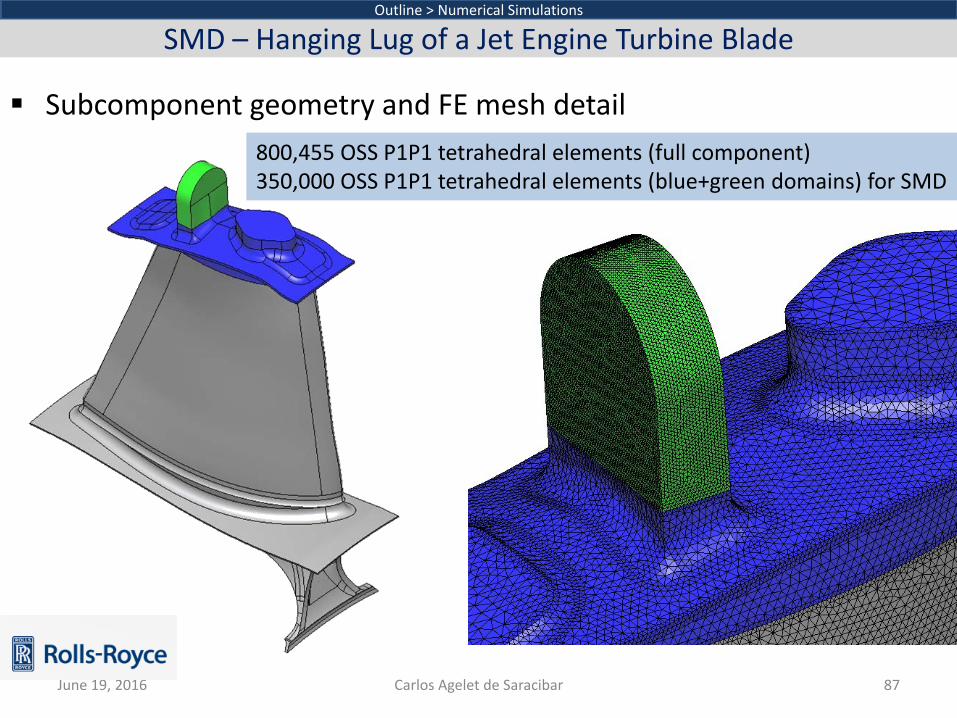
Subcomponent geometry and FE mesh detail
June 19, 2016 Carlos Agelet de Saracibar 87
Outline > Numerical Simulations
SMD – Hanging Lug of a Jet Engine Turbine Blade
800,455 OSS P1P1 tetrahedral elements (full component) 350,000 OSS P1P1 tetrahedral elements (blue+green domains) for SMD
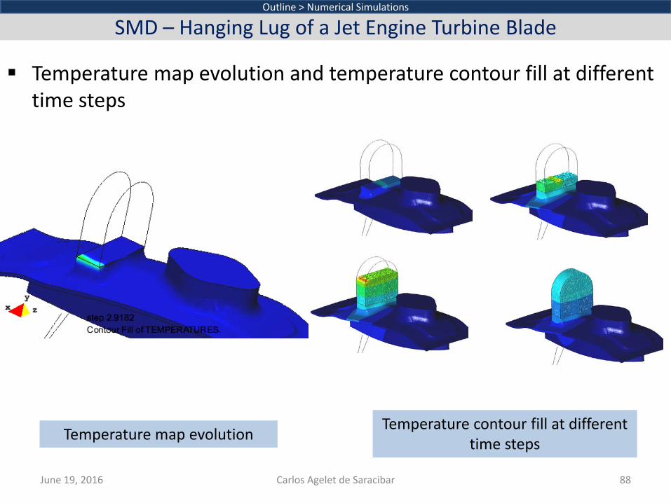
Temperature map evolution and temperature contour fill at different time steps
June 19, 2016 Carlos Agelet de Saracibar 88
Outline > Numerical Simulations
SMD – Hanging Lug of a Jet Engine Turbine Blade
Temperature map evolution Temperature contour fill at different time steps
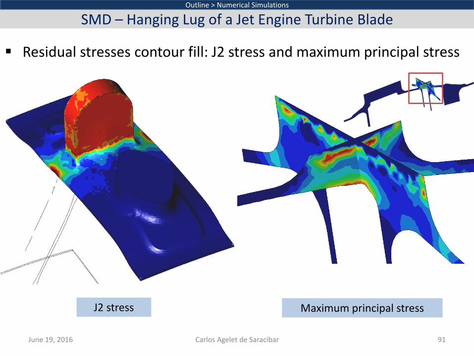
Residual stresses contour fill: J2 stress and maximum principal stress
June 19, 2016 Carlos Agelet de Saracibar 91
Outline > Numerical Simulations
SMD – Hanging Lug of a Jet Engine Turbine Blade
J2 stress Maximum principal stress
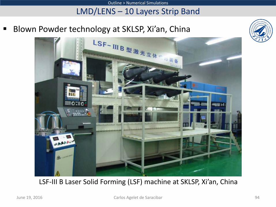
Blown Powder technology at SKLSP, Xi’an, China LSF-III B Laser Solid Forming (LSF) machine at SKLSP, Xi’an, China
June 19, 2016 Carlos Agelet de Saracibar 94
Outline > Numerical Simulations
LMD/LENS – 10 Layers Strip Band
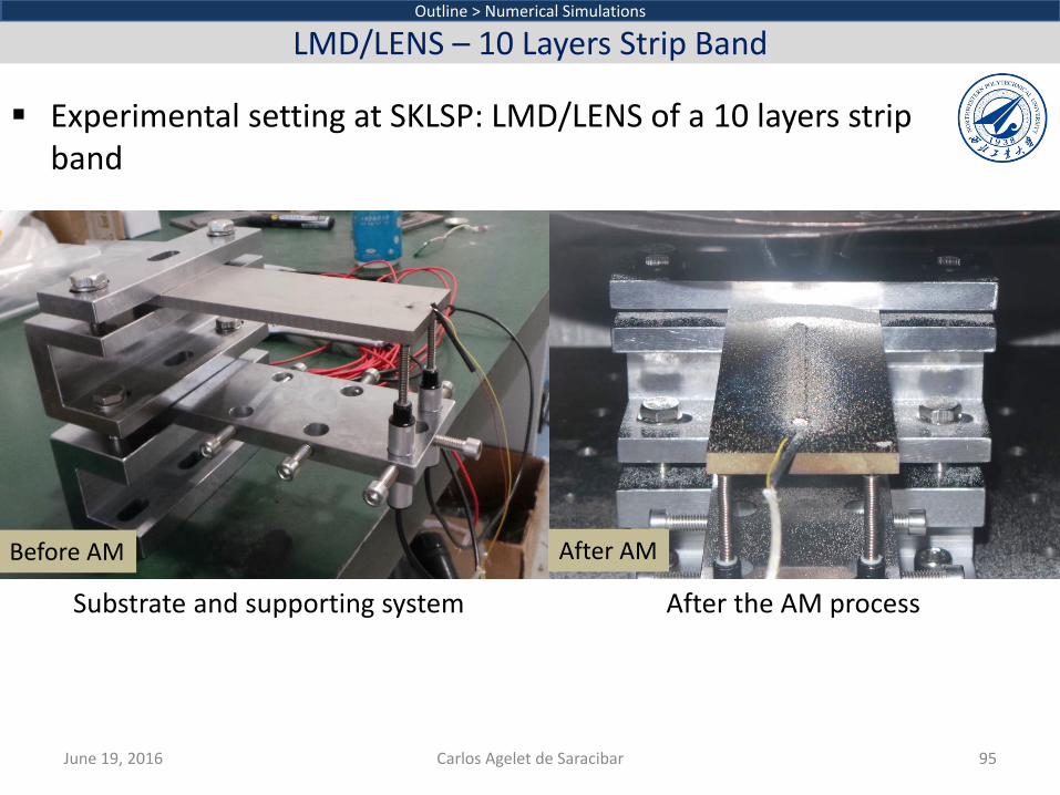
Experimental setting at SKLSP: LMD/LENS of a 10 layers strip band
June 19, 2016 Carlos Agelet de Saracibar 95
Outline > Numerical Simulations
LMD/LENS – 10 Layers Strip Band
Substrate and supporting system After the AM process
Before AM After AM
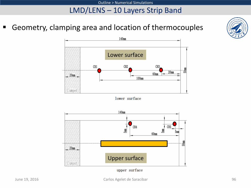
Geometry, clamping area and location of thermocouples
June 19, 2016 Carlos Agelet de Saracibar 96
Outline > Numerical Simulations
LMD/LENS – 10 Layers Strip Band
Lower surface
Upper surface
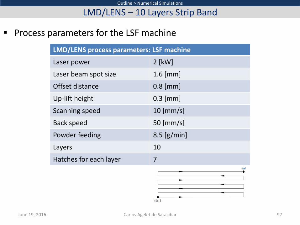
Process parameters for the LSF machine
June 19, 2016 Carlos Agelet de Saracibar 97
Outline > Numerical Simulations
LMD/LENS – 10 Layers Strip Band
LMD/LENS process parameters: LSF machine
Laser power 2 [kW]
Laser beam spot size 1.6 [mm]
Offset distance 0.8 [mm]
Up-lift height 0.3 [mm]
Scanning speed 10 [mm/s]
Back speed 50 [mm/s]
Powder feeding 8.5 [g/min]
Layers 10
Hatches for each layer 7

Process parameters used in the LMD/LENS numerical simulation
June 19, 2016 Carlos Agelet de Saracibar 98
Outline > Numerical Simulations
LMD/LENS – 10 Layers Strip Band
LMD/LENS process parameters: Numerical simulation
Laser power 2 [kW]
Power absorption 16.5 %
Scanning speed 10 [mm/s]
Back speed 50 [mm/s]
Penetration 0.28 [mm]
Layer thickness 0.28 [mm]
Layer width 1.75 [mm]
Overlapping 50 %
Layers 10
Hatches for each layer 7
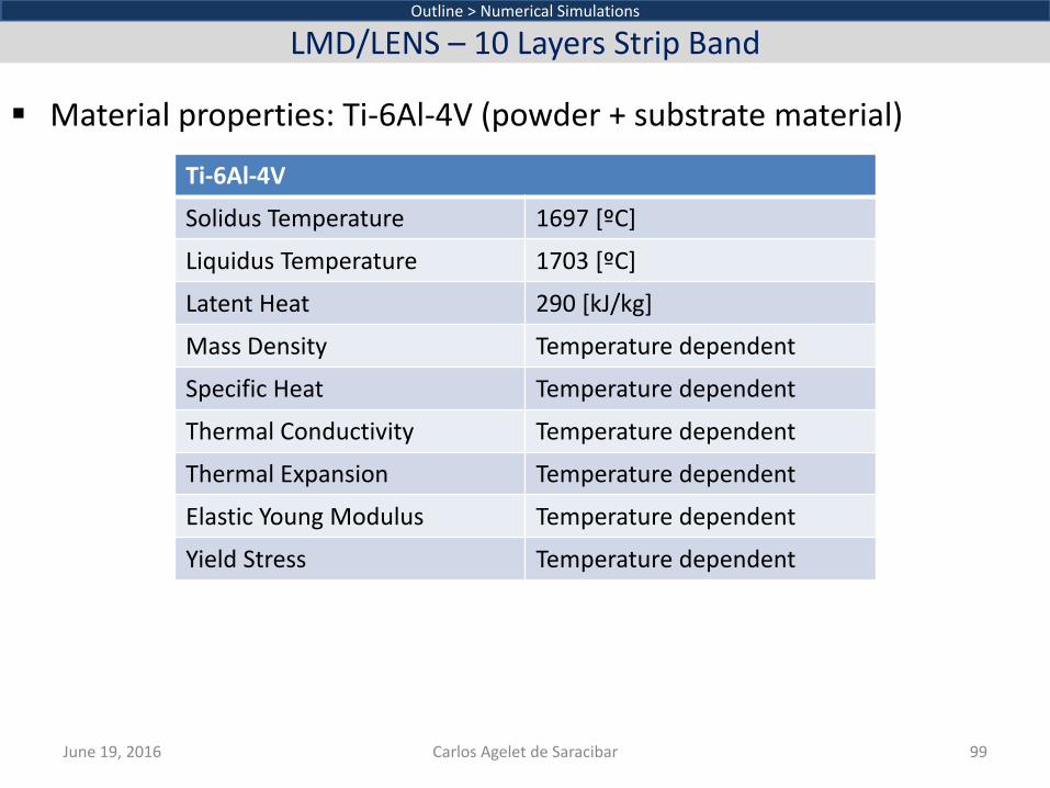
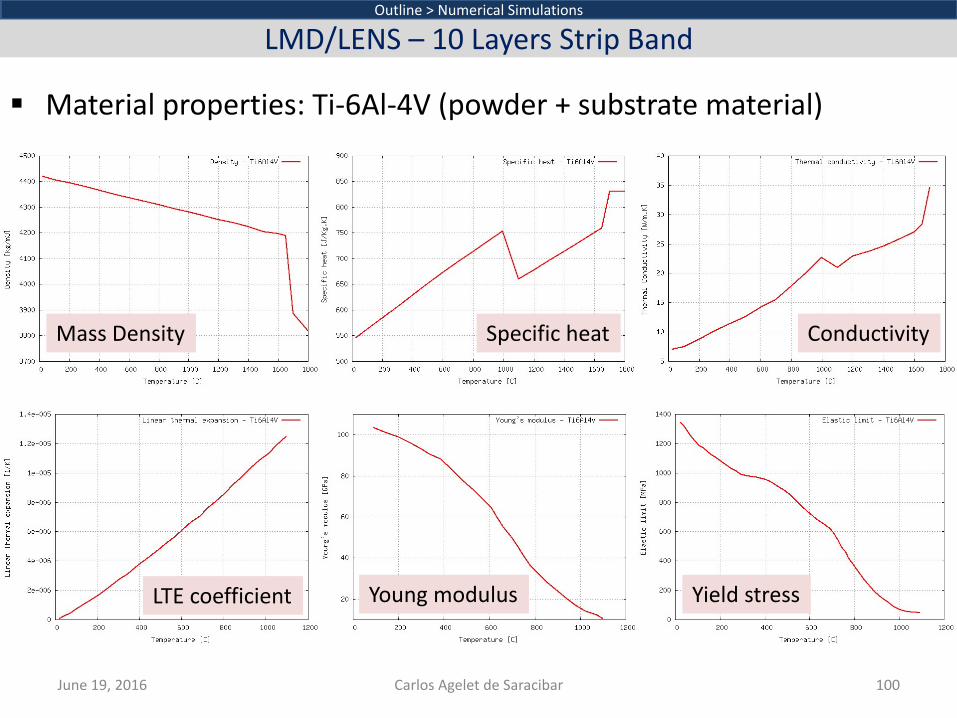
Material properties: Ti-6Al-4V (powder + substrate material)
June 19, 2016 Carlos Agelet de Saracibar 99
Outline > Numerical Simulations
LMD/LENS – 10 Layers Strip Band
Ti-6Al-4V
Solidus Temperature 1697 [ºC]
Liquidus Temperature 1703 [ºC]
Latent Heat 290 [kJ/kg]
Mass Density Temperature dependent
Specific Heat Temperature dependent
Thermal Conductivity Temperature dependent
Thermal Expansion Temperature dependent
Elastic Young Modulus Temperature dependent
Yield Stress Temperature dependent
Material properties: Ti-6Al-4V (powder + substrate material)
June 19, 2016 Carlos Agelet de Saracibar 100
Outline > Numerical Simulations
LMD/LENS – 10 Layers Strip Band
Mass Density Conductivity Specific heat
Yield stress LTE coefficient Young modulus
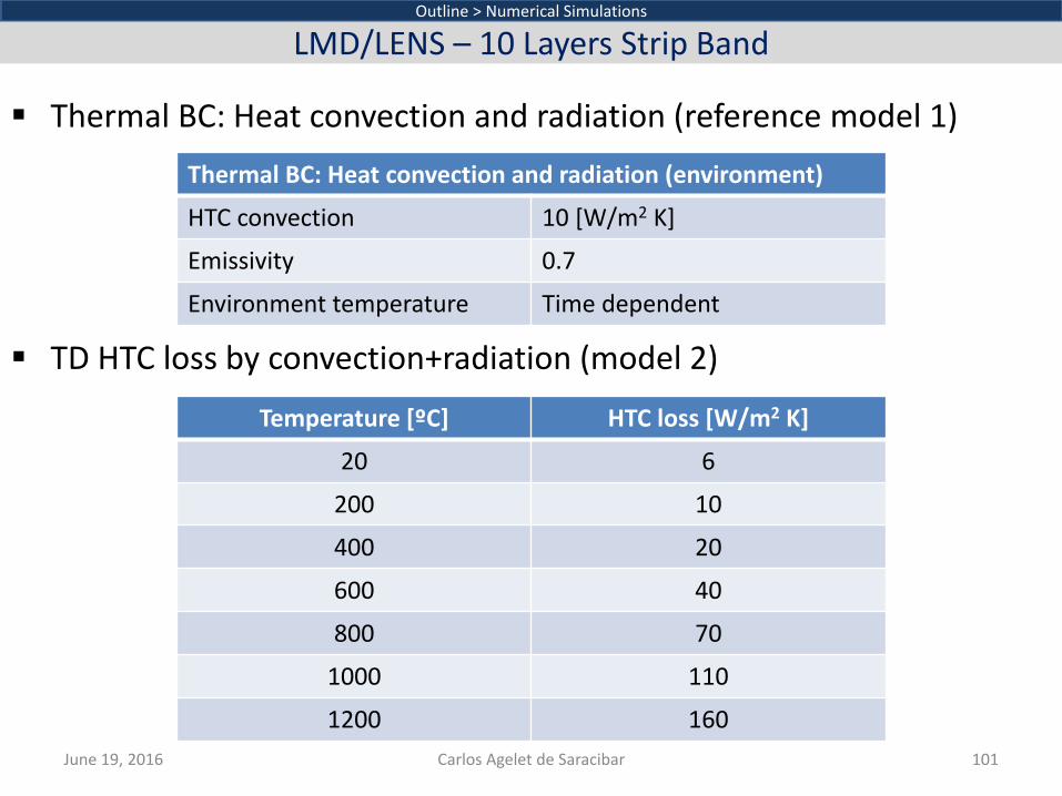
Thermal BC: Heat convection and radiation (reference model 1)
TD HTC loss by convection+radiation (model 2)
June 19, 2016 Carlos Agelet de Saracibar 101
Outline > Numerical Simulations
LMD/LENS – 10 Layers Strip Band
Thermal BC: Heat convection and radiation (environment)
HTC convection 10 [W/m2 K]
Emissivity 0.7
Environment temperature Time dependent
Temperature [ºC] HTC loss [W/m2 K]
20 6
200 10
400 20
600 40
800 70
1000 110
1200 160
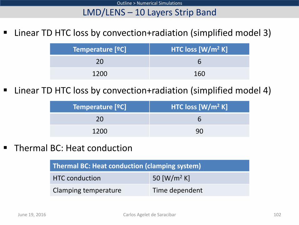
Linear TD HTC loss by convection+radiation (simplified model 3)
Linear TD HTC loss by convection+radiation (simplified model 4)
Thermal BC: Heat conduction
June 19, 2016 Carlos Agelet de Saracibar 102
Outline > Numerical Simulations
LMD/LENS – 10 Layers Strip Band
Temperature [ºC] HTC loss [W/m2 K]
20 6
1200 160
Temperature [ºC] HTC loss [W/m2 K]
20 6
1200 90
Thermal BC: Heat conduction (clamping system)
HTC conduction 50 [W/m2 K]
Clamping temperature Time dependent
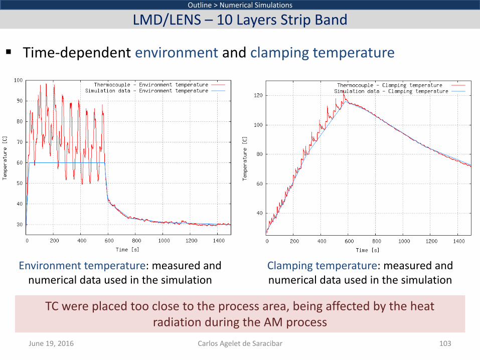
Time-dependent environment and clamping temperature
June 19, 2016 Carlos Agelet de Saracibar 103
Outline > Numerical Simulations
LMD/LENS – 10 Layers Strip Band
Environment temperature: measured and numerical data used in the simulation
Clamping temperature: measured and numerical data used in the simulation
TC were placed too close to the process area, being affected by the heat radiation during the AM process
FE mesh
June 19, 2016 Carlos Agelet de Saracibar 104
Outline > Numerical Simulations
LMD/LENS – 10 Layers Strip Band
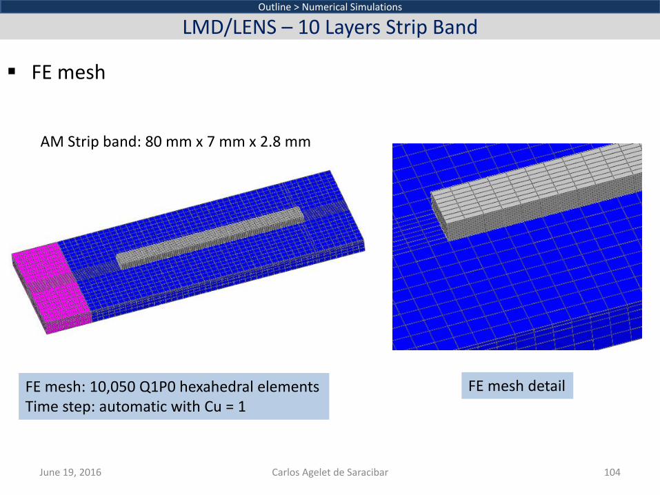
FE mesh detail
AM Strip band: 80 mm x 7 mm x 2.8 mm
FE mesh: 10,050 Q1P0 hexahedral elements Time step: automatic with Cu = 1
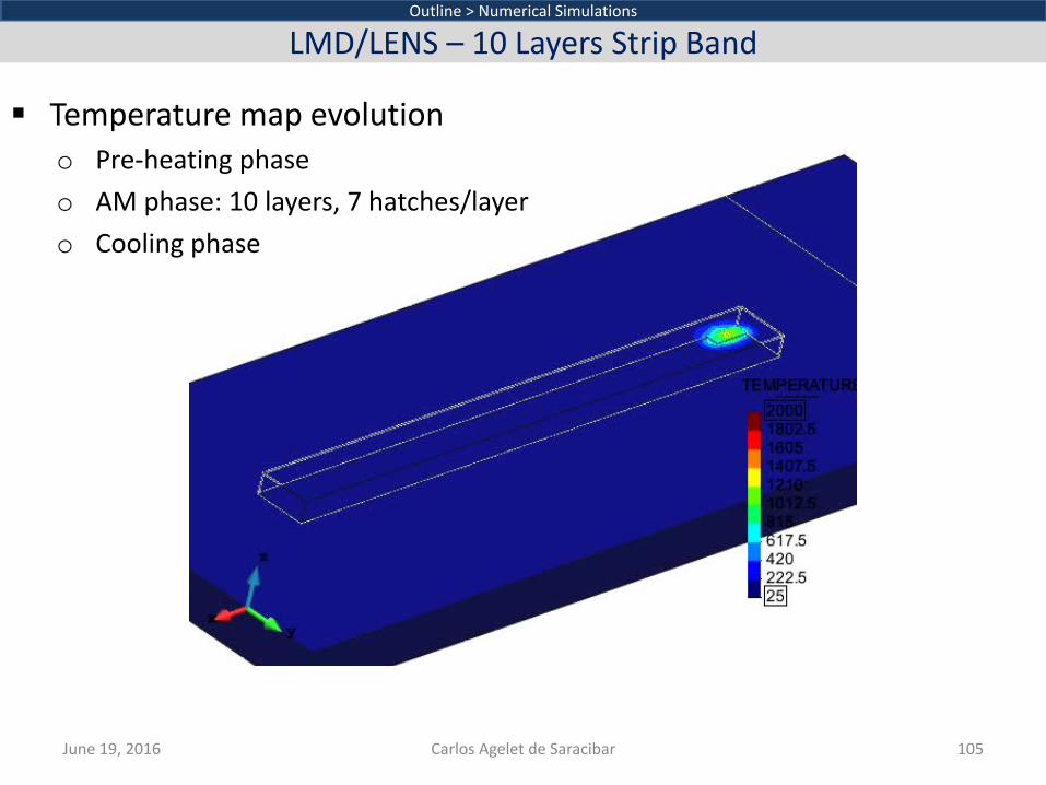
Temperature map evolution o Pre-heating phase o AM phase: 10 layers, 7 hatches/layer o Cooling phase
June 19, 2016 Carlos Agelet de Saracibar 105
Outline > Numerical Simulations
LMD/LENS – 10 Layers Strip Band
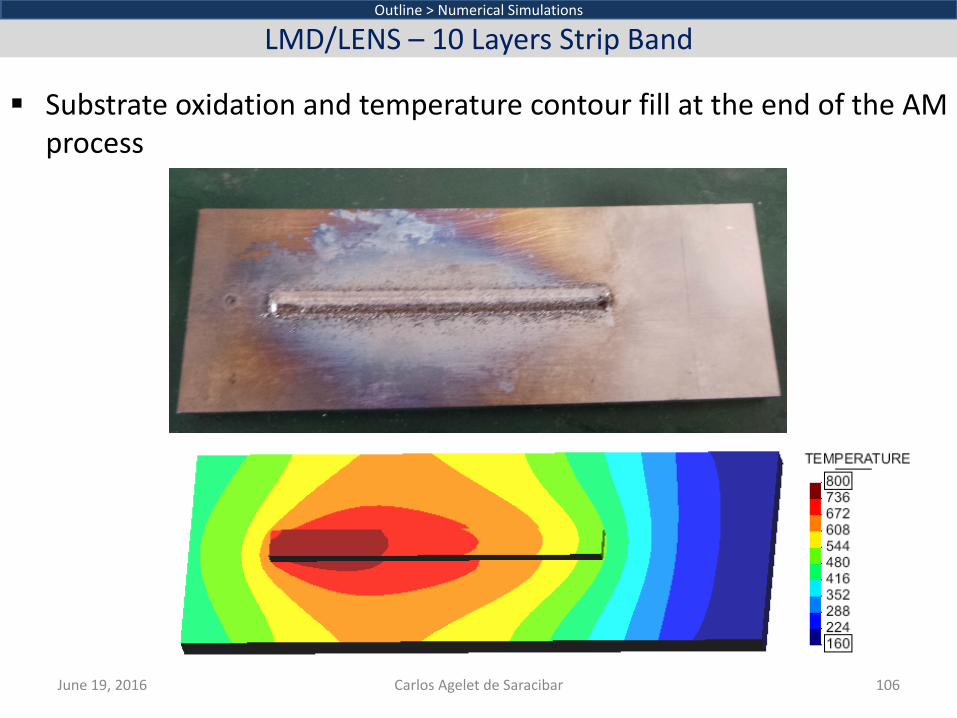
Substrate oxidation and temperature contour fill at the end of the AM process
June 19, 2016 Carlos Agelet de Saracibar 106
Outline > Numerical Simulations
LMD/LENS – 10 Layers Strip Band

Temperature evolution at TC CH1-CH3: lower surface
June 19, 2016 Carlos Agelet de Saracibar 107
Outline > Numerical Simulations
LMD/LENS – 10 Layers Strip Band
Zoom box Numerical
Experimental
Experimental Numerical
Very good agreement between numerical and experimental temperature evolution at TC
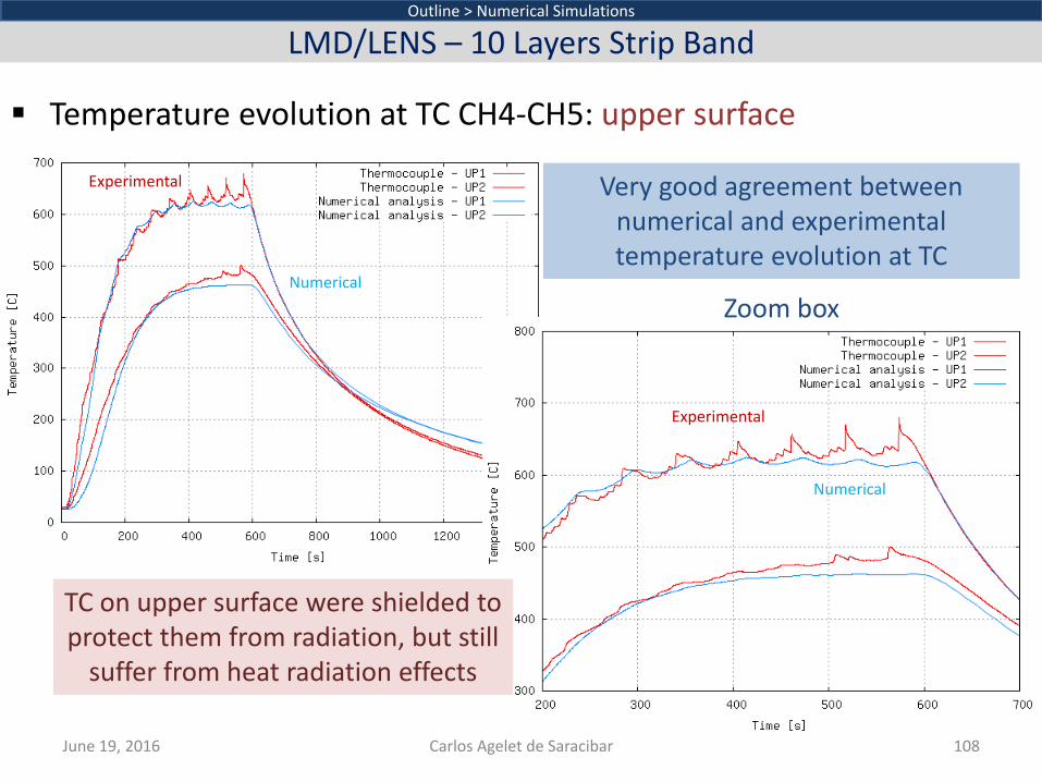
Temperature evolution at TC CH4-CH5: upper surface
June 19, 2016 Carlos Agelet de Saracibar 108
Outline > Numerical Simulations
LMD/LENS – 10 Layers Strip Band
Zoom box Numerical
Experimental
Experimental
Numerical
Very good agreement between numerical and experimental temperature evolution at TC
TC on upper surface were shielded to protect them from radiation, but still
suffer from heat radiation effects
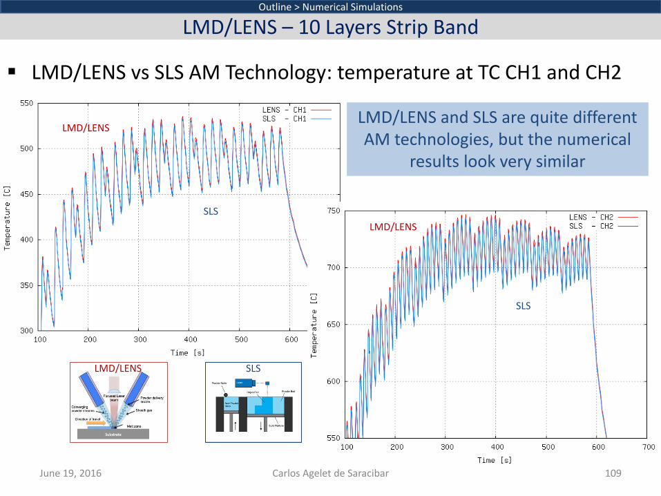
LMD/LENS vs SLS AM Technology: temperature at TC CH1 and CH2
June 19, 2016 Carlos Agelet de Saracibar 109
Outline > Numerical Simulations
LMD/LENS – 10 Layers Strip Band
SLS
LMD/LENS
LMD/LENS
SLS
LMD/LENS and SLS are quite different AM technologies, but the numerical
results look very similar
LMD/LENS SLS
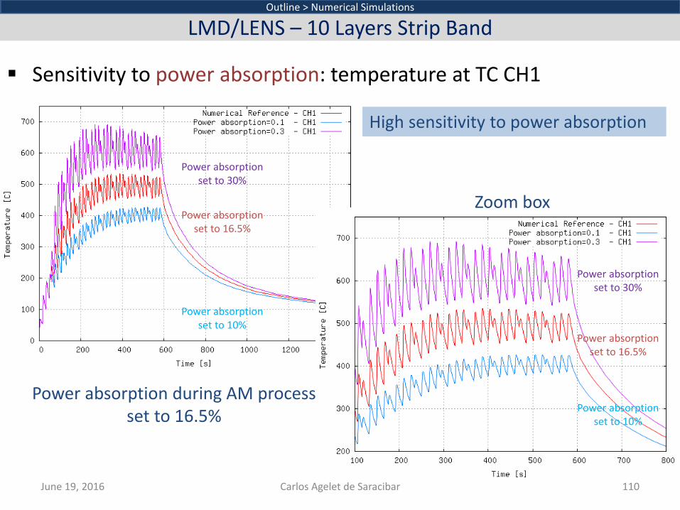
Sensitivity to power absorption: temperature at TC CH1
June 19, 2016 Carlos Agelet de Saracibar 110
Outline > Numerical Simulations
LMD/LENS – 10 Layers Strip Band
Power absorption during AM process set to 16.5%
Power absorption set to 30%
Power absorption set to 10%
Power absorption set to 10%
Power absorption set to 16.5%
Power absorption set to 30%
Power absorption set to 16.5%
Zoom box
High sensitivity to power absorption

Sensitivity to pre-heating phase: temperature at TC CH2
June 19, 2016 Carlos Agelet de Saracibar 111
Outline > Numerical Simulations
LMD/LENS – 10 Layers Strip Band
Power absorption during AM phase set to 16.5%, while during pre-
heating phase is set to 10%
Zoom box
Cooling
Without pre-heating
With pre-heating
AM
Pre-
heat
ing
Without pre-heating
With pre-heating
Pre-heating shows a lower power absorption
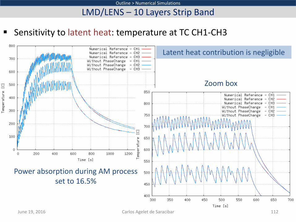
Sensitivity to latent heat: temperature at TC CH1-CH3
June 19, 2016 Carlos Agelet de Saracibar 112
Outline > Numerical Simulations
LMD/LENS – 10 Layers Strip Band
Latent heat contribution is negligible
Zoom box
Power absorption during AM process set to 16.5%
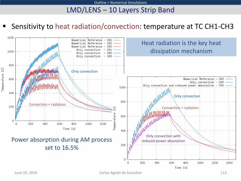
Sensitivity to heat radiation/convection: temperature at TC CH1-CH3
June 19, 2016 Carlos Agelet de Saracibar 113
Outline > Numerical Simulations
LMD/LENS – 10 Layers Strip Band
Power absorption during AM process set to 16.5%
Only convection
Convection + radiation
Only convection
Convection + radiation
Only convection with reduced power absorption
Heat radiation is the key heat dissipation mechanism
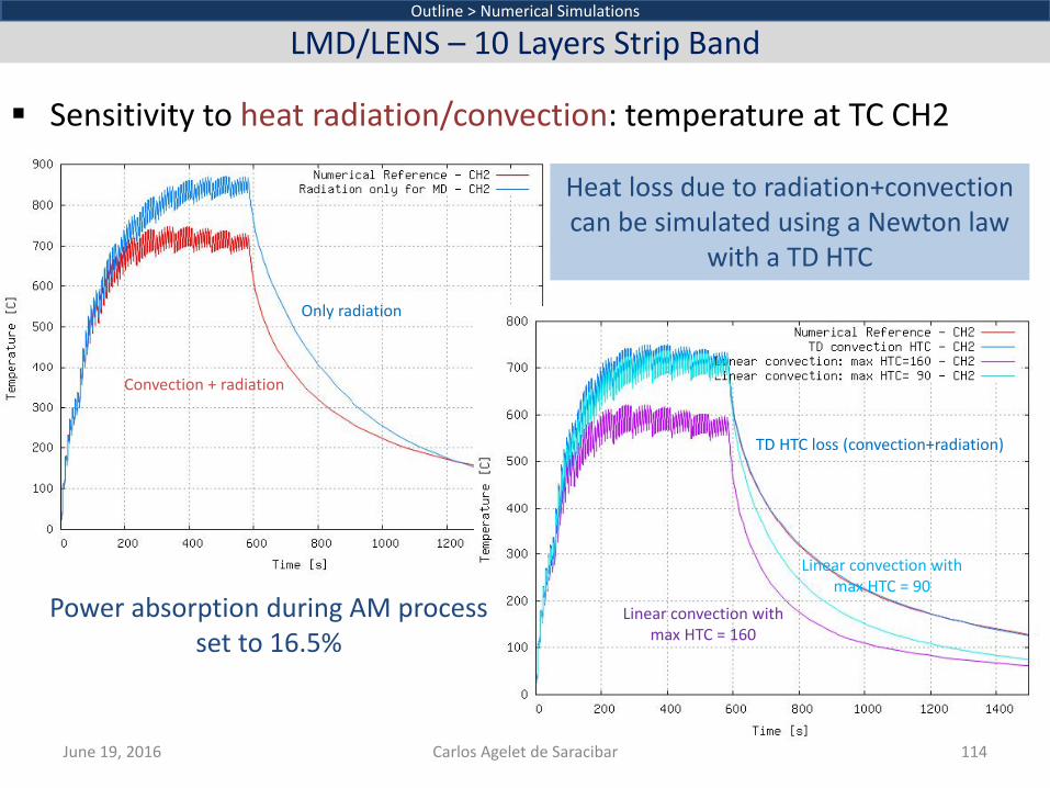
Sensitivity to heat radiation/convection: temperature at TC CH2
June 19, 2016 Carlos Agelet de Saracibar 114
Outline > Numerical Simulations
LMD/LENS – 10 Layers Strip Band
Only radiation
Convection + radiation
TD HTC loss (convection+radiation)
Linear convection with max HTC = 160
Linear convection with max HTC = 90
Heat loss due to radiation+convection can be simulated using a Newton law
with a TD HTC
Power absorption during AM process set to 16.5%
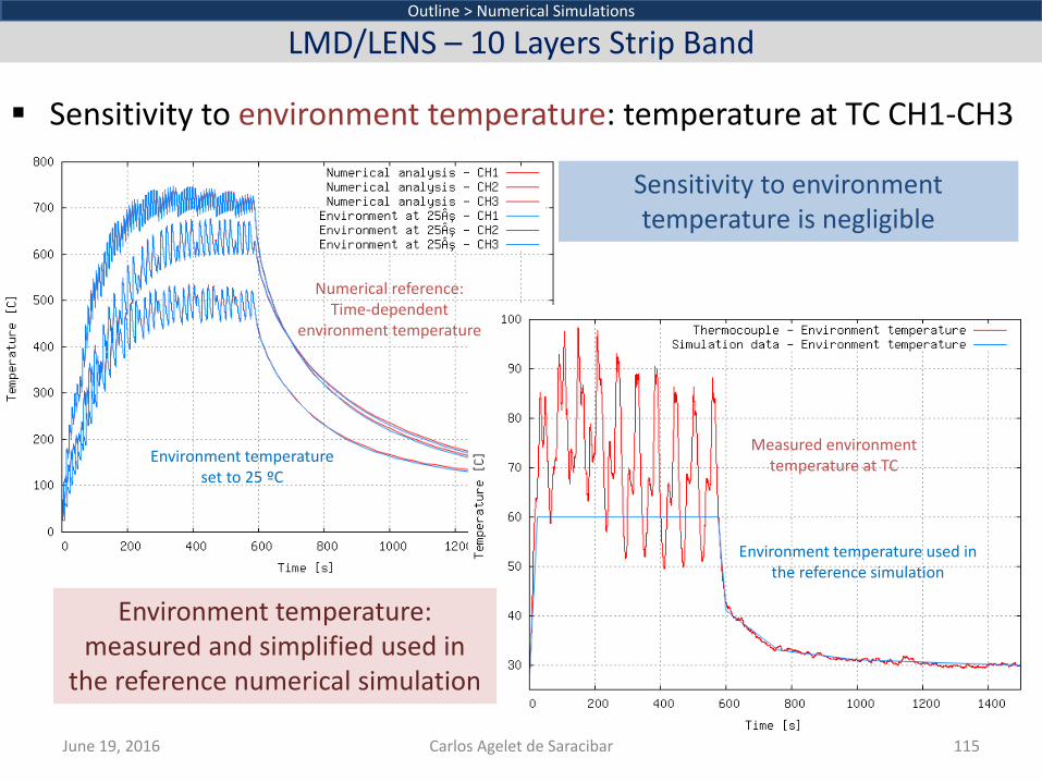
Sensitivity to environment temperature: temperature at TC CH1-CH3
June 19, 2016 Carlos Agelet de Saracibar 115
Outline > Numerical Simulations
LMD/LENS – 10 Layers Strip Band
Environment temperature set to 25 ºC
Measured environment temperature at TC
Environment temperature used in the reference simulation
Sensitivity to environment temperature is negligible
Environment temperature: measured and simplified used in
the reference numerical simulation
Numerical reference: Time-dependent
environment temperature
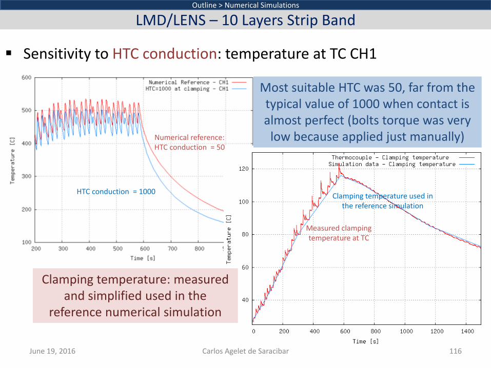
Sensitivity to HTC conduction: temperature at TC CH1
June 19, 2016 Carlos Agelet de Saracibar 116
Outline > Numerical Simulations
LMD/LENS – 10 Layers Strip Band
HTC conduction = 1000
Most suitable HTC was 50, far from the typical value of 1000 when contact is almost perfect (bolts torque was very
low because applied just manually)
Clamping temperature: measured and simplified used in the
reference numerical simulation
Numerical reference: HTC conduction = 50
Measured clamping temperature at TC
Clamping temperature used in the reference simulation
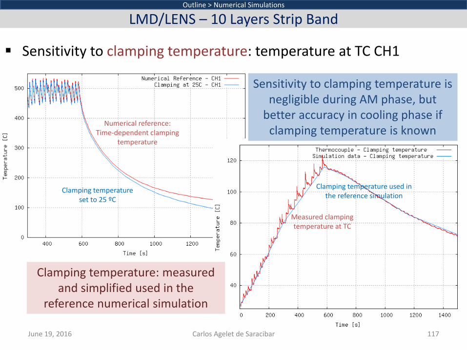
Sensitivity to clamping temperature: temperature at TC CH1
June 19, 2016 Carlos Agelet de Saracibar 117
Outline > Numerical Simulations
LMD/LENS – 10 Layers Strip Band
Clamping temperature set to 25 ºC
Measured clamping temperature at TC
Clamping temperature used in the reference simulation
Sensitivity to clamping temperature is negligible during AM phase, but
better accuracy in cooling phase if clamping temperature is known
Clamping temperature: measured and simplified used in the
reference numerical simulation
Numerical reference: Time-dependent clamping
temperature
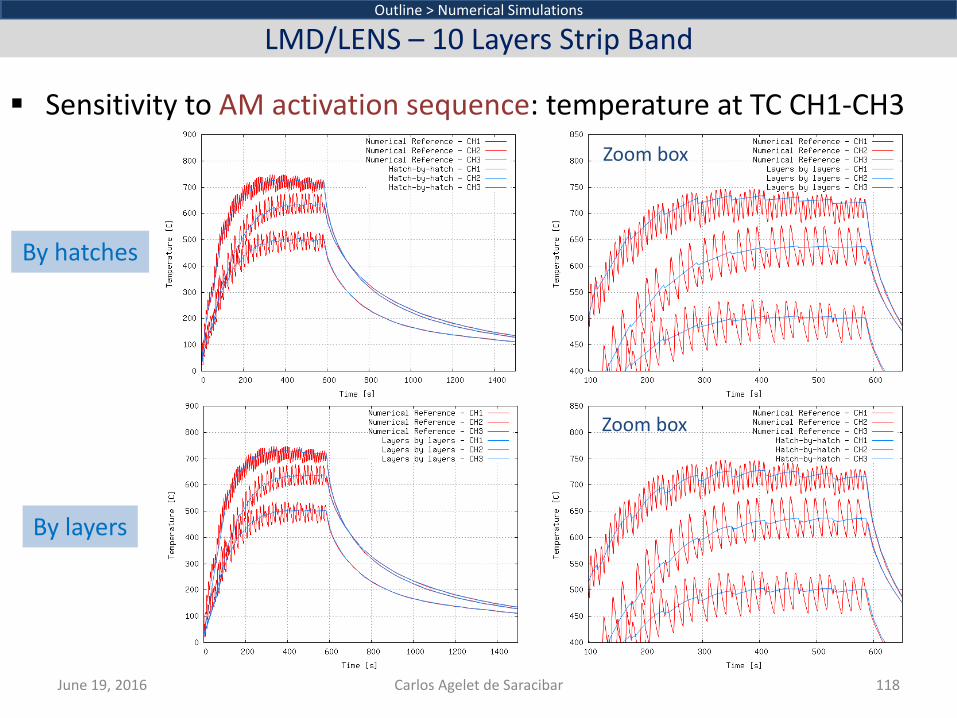
Sensitivity to AM activation sequence: temperature at TC CH1-CH3
June 19, 2016 Carlos Agelet de Saracibar 118
Outline > Numerical Simulations
LMD/LENS – 10 Layers Strip Band
By hatches
By layers
Zoom box
Zoom box
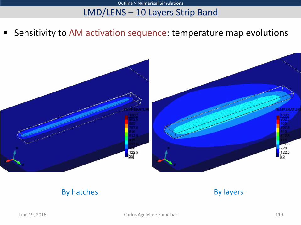
Sensitivity to AM activation sequence: temperature map evolutions
June 19, 2016 Carlos Agelet de Saracibar 119
Outline > Numerical Simulations
LMD/LENS – 10 Layers Strip Band
By hatches By layers
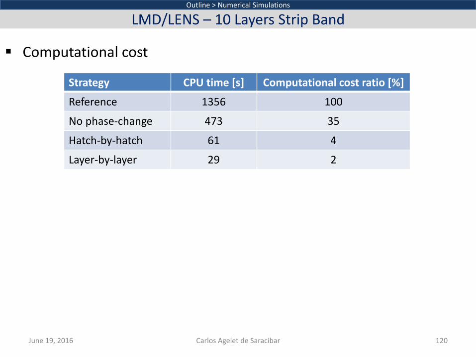
Computational cost
June 19, 2016 Carlos Agelet de Saracibar 120
Outline > Numerical Simulations
LMD/LENS – 10 Layers Strip Band
Strategy CPU time [s] Computational cost ratio [%]
Reference 1356 100
No phase-change 473 35
Hatch-by-hatch 61 4
Layer-by-layer 29 2
Introduction Problem statement Computational model Numerical simulations Concluding remarks
Outline > Concluding Remarks
Concluding Remarks
June 19, 2016 Carlos Agelet de Saracibar 121
Remarkable accuracy in the numerical simulation of DED AM technologies (wire-feed SMD and blown powder LMD/LENS), has been achieved
June 19, 2016 Carlos Agelet de Saracibar 122
Outline > Concluding Remarks
Concluding Remarks
High sensitivity to power absorption. Power absorption for blown powder (LMD/LENS) technology, is very low (around 15% of the power input). Pre-heating phase shows a lower power absorption (around 10% of the power input)
Latent heat of fusion contribution due to liquid-solid phase-change can be neglected, saving up to a 65% of the total CPU time
Heat radiation is the key mechanism to dissipate heat through the boundaries with the environment. It cannot be neglected, but Stefan-Boltzmann law can be replaced by a Newton law using a TD HTC. Total heat loss by convection + radiation can be conveniently simulated using a single Newton law with a TD HTC
Most suitable HTC by conduction at the clamping system was 50 W/m2 K, being far from the typical value of 1000 W/m2 K when contact is almost perfect. This can be explained by the fact that the bolts torque was very low because applied just manually
June 19, 2016 Carlos Agelet de Saracibar 123
Outline > Concluding Remarks
Concluding Remarks
Time variation of the environment (closed chamber) temperature and clamping system temperature can be neglected. Nevertheless, better accuracy can be achieved in the cooling phase if the time-dependent clamping temperature is available
CPU time can be drastically reduced using a hatch-by-hatch or even a layer-by-layer AM activation sequence. Average temperature evolution can be well captured, but the accuracy on the local thermal history is lost, and the mechanical response can be compromised
Efficient Manufacturing for Aerospace Components Using Additive Manufacturing, Net Shape HIP and Investment Casting (EMUSIC), H2020-MG-2015_SingleStage-A, Project no. 690725, EC
Computer Aided Technologies for Additive Manufacturing (CAxMan), H2020-FoF-2015_CNECT, Project no. 680448, EC
Computational Cloud Services and Workflows for Agile Engineering. HPC Workflow for Simulation of Additive Manufacturing for Improving the Production of Gearboxes (CLOUDFLOW), CloudFlow-2, Project no. 609100, EC
Virtual Engineering for Robust Manufacturing with Design Integration (VERDI), FP6-2003-AERO-1, AST4-CT-2005-516046, Project no. 516046, EC
State Administration of Foreign Experts Affairs of China through the High-end Experts Recruitment Program
National Natural Science Foundation of China, Grants 51323008 and 51271213 National Basic Research Program of China, Grant 2011CB610402 National High Technology Research and Development Program of China, Grant
2013AA031103 Specialized Research Fund for the Doctoral Program of Higher Education of China, Grant
20116102110016 Yasmine Lebbar
June 19, 2016 Carlos Agelet de Saracibar 124
Outline > Acknowledgments
Acknowledgments

June 19, 2016 Carlos Agelet de Saracibar 125
On the Numerical Simulation of AM Processes M. Chiumenti1,2, M. Cervera1, N. Dialami1, C. Agelet de Saracibar1 1 International Center for Numerical Methods in Engineering (CIMNE) UPC BarcelonaTech, Barcelona, Spain W. Huang2, X. Lin2, L. Wei2, Y. Zheng2, L. Ma2 2 State Key Laboratory of Solidification Processing (SKLSP) Northwestern Polytechnical University (NWPU), Xi’an, China
2nd International Conference on Computational Methods in Manufacturing Processes Liège, Belgium, 18-20 May 2016
ICOMP 2016