Mathematical Modeling With Maple

04/18/2023 SFR COLLEGE PRESENTATION 1

MATHEMATICAL MODELING WITH MAPLE

ByDr. V.GNANARAJ

ASSOCIATE PROFESSOR IN MATHEMATICSTHIAGARAJAR COLLEGE OF ENGINEERING

MADURAI


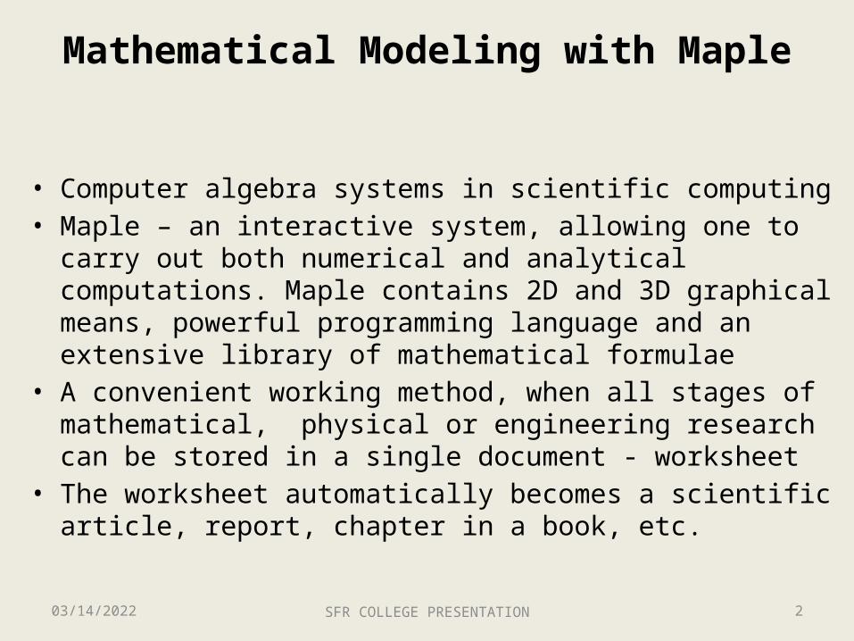
Mathematical Modeling with Maple

• Computer algebra systems in scientific computing • Maple – an interactive system, allowing one to carry out both

numerical and analytical computations. Maple contains 2D and 3D graphical means, powerful programming language and an extensive library of mathematical formulae

• A convenient working method, when all stages of mathematical, physical or engineering research can be stored in a single document - worksheet

• The worksheet automatically becomes a scientific article, report, chapter in a book, etc.


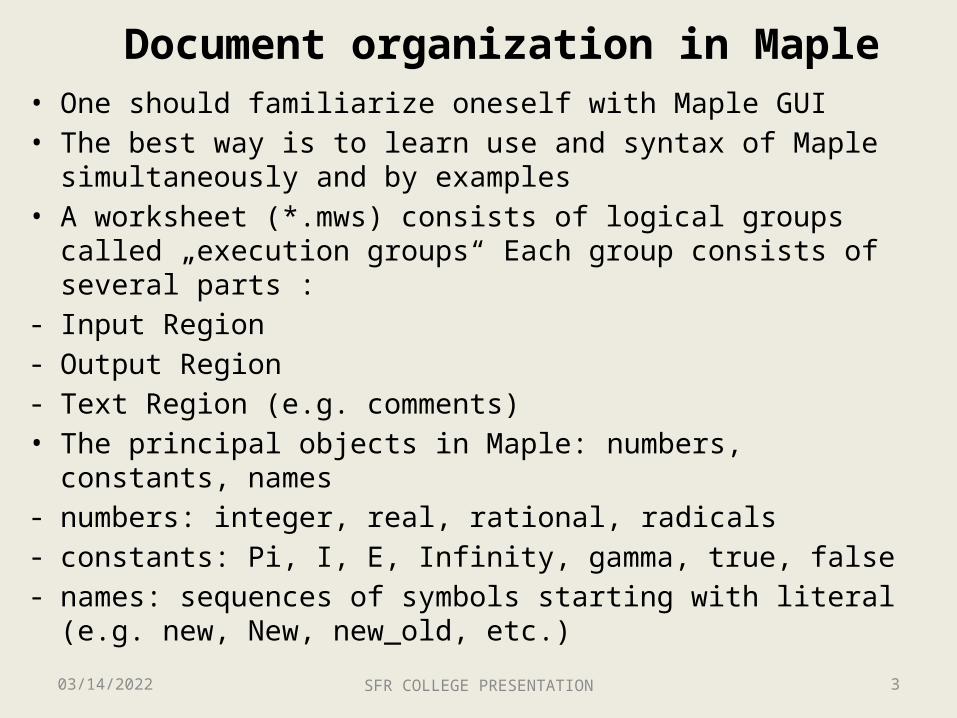
Document organization in Maple• One should familiarize oneself with Maple GUI• The best way is to learn use and syntax of Maple simultaneously

and by examples• A worksheet (*.mws) consists of logical groups called „execution

groups“ Each group consists of several parts :- Input Region - Output Region- Text Region (e.g. comments)• The principal objects in Maple: numbers, constants, names- numbers: integer, real, rational, radicals- constants: Pi, I, E, Infinity, gamma, true, false- names: sequences of symbols starting with literal (e.g. new, New,

new_old, etc.)


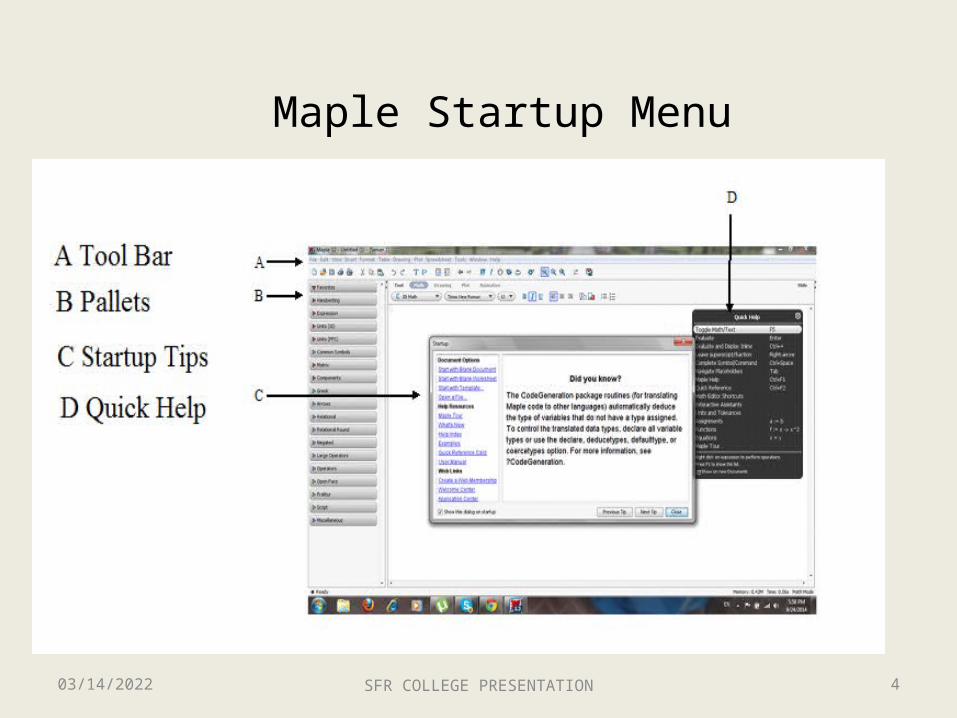
Maple Startup Menu


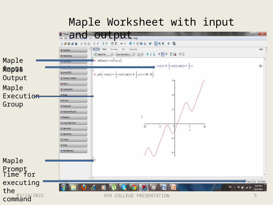
Maple Worksheet with input and output

Maple InputMaple Output

Maple Execution Group

Maple Prompt

Time for executing the command


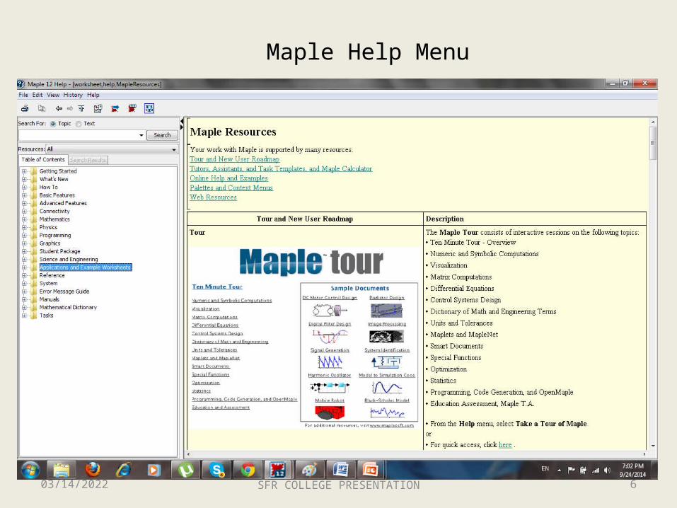
Maple Help Menu


Syntax and expressions

• After typing a command, you should inform the computer that the command has ended and must be accepted. There are two types of terminators: ; and : The colon is needed to suppress Return – the output is not printed

• The symbol % is called “ditto”, it is used to refer to previous return. Twofold ditto (%%) refers to the second last return, etc

• Expressions are the main object for the most of commands. Expressions are composed of constants, variables, signs of arithmetical and logical operations


Typical syntax errors and remedies

• Forgetting a bracket or an operator – the error message comes after Return (sometimes it appears meaningless)

• It is easier to type the brackets and some operators first, and then insert functions, variables and parameters, e.g.

> ( )*(sqrt( ) + ( )^( ) )* exp( );• It is better to start a new worksheet with the command restart –

this resets the system and variables used in a previous worksheet do not cast their value into the new one

• Not all combinations of symbols are allowed in Maple (e.g. Pi and I are already used by the system


Solving equations with Maple• Two different methods of finding roots:

1) analytical (symbolic); 2)numerical • Maple provides two respective built-in functions:

1) solve; 2) fsolve• Analytical approach: the equation is manipulated up to the form

when the unknown is expressed in terms of the knowns – solve operates in this way. The variety of equations to be analytically solved is determined by the set of techniques available in Maple

• Each new Maple version – new commands and packages. Multipurpose commands of the xsolve type: dsolve for ODE, pdsolve for PDE, rsolve for difference equations

• New libraries: DEtools, PDEtools, LREtools. Special packages for implicit solutions: DESol, RESol (difference), RootOf (algebra)


Analytical solutions

• The solve command – multipurpose, can be applied to systems of algebraic equations, inequalities, functional equations, identities. The form: solve (eqn, var), where eqn is an equation or a system of equations, var is a variable or a group of variables. If the latter parameter is absent, solve will look for solutions with respect to all symbolic variables

• The system of equations and the group of variables are given as sets (in curly brackets and separated by commas)

• Example: > s:=solve({6*x+y=8, 3*x-2*y=4},{x,y});• If the equation is written without the equality sign it is viewed as

one part of the equality, the other being considered zero:

> sl:=solve(x^7+8*x,x);


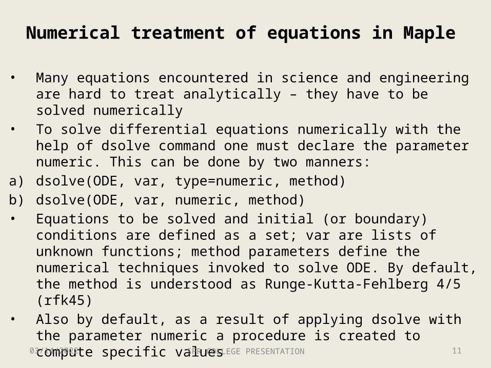
• Many equations encountered in science and engineering are hard to treat analytically – they have to be solved numerically

• To solve differential equations numerically with the help of dsolve command one must declare the parameter numeric. This can be done by two manners:

a) dsolve(ODE, var, type=numeric, method)b) dsolve(ODE, var, numeric, method)• Equations to be solved and initial (or boundary) conditions are

defined as a set; var are lists of unknown functions; method parameters define the numerical techniques invoked to solve ODE. By default, the method is understood as Runge-Kutta-Fehlberg 4/5 (rfk45)

• Also by default, as a result of applying dsolve with the parameter numeric a procedure is created to compute specific values

Numerical treatment of equations in Maple


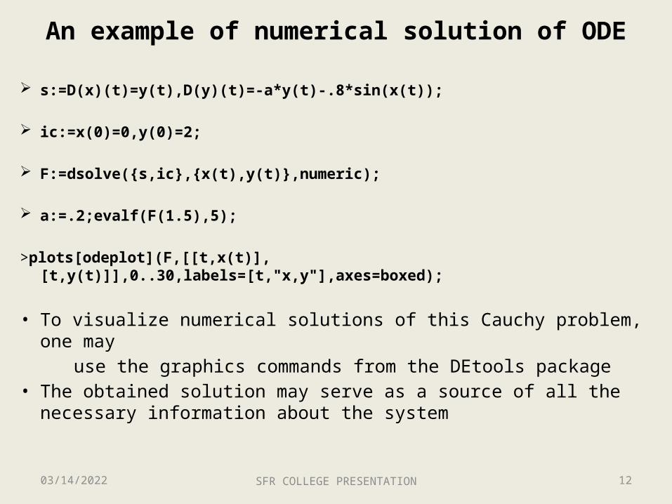
s:=D(x)(t)=y(t),D(y)(t)=-a*y(t)-.8*sin(x(t));

ic:=x(0)=0,y(0)=2;

F:=dsolve({s,ic},{x(t),y(t)},numeric);

a:=.2;evalf(F(1.5),5);

>plots[odeplot](F,[[t,x(t)],[t,y(t)]],0..30,labels=[t,"x,y"],axes=boxed);

• To visualize numerical solutions of this Cauchy problem, one may

use the graphics commands from the DEtools package• The obtained solution may serve as a source of all the necessary

information about the system

An example of numerical solution of ODE


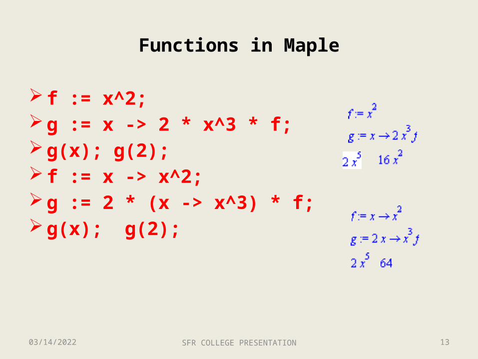
Functions in Maple

f := x^2; g := x -> 2 * x^3 * f; g(x); g(2); f := x -> x^2; g := 2 * (x -> x^3) * f; g(x); g(2);


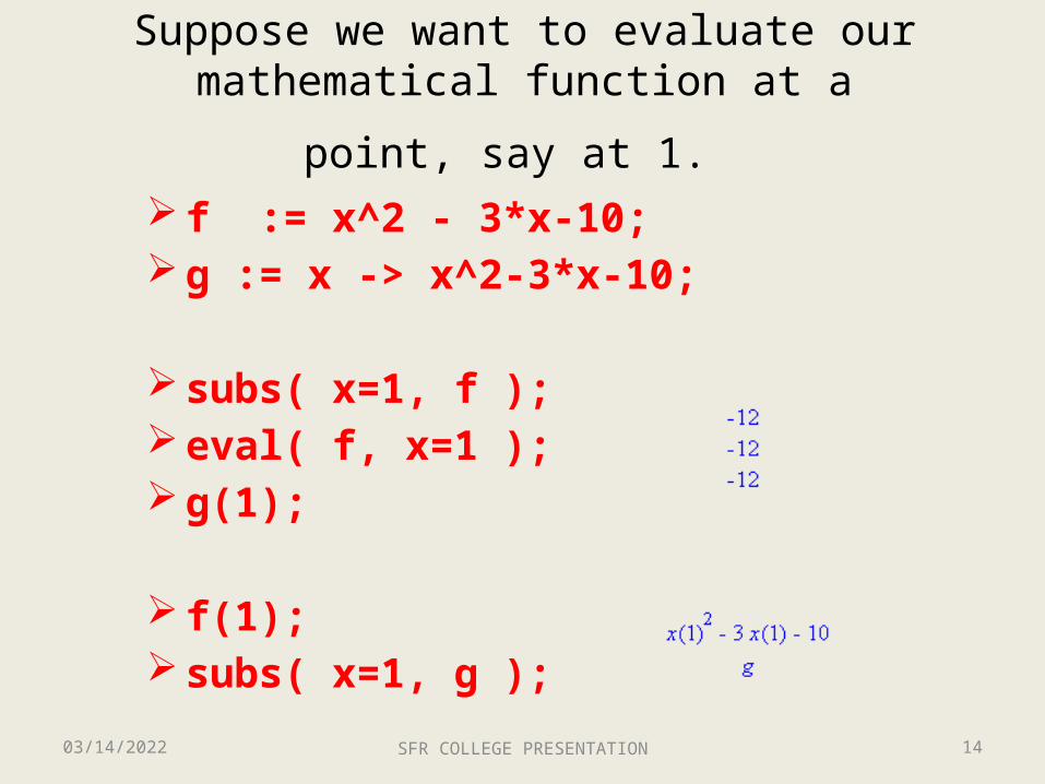
Suppose we want to evaluate our

mathematical function at a point, say at 1. f := x^2 - 3*x-10; g := x -> x^2-3*x-10;

subs( x=1, f ); eval( f, x=1 ); g(1);

f(1); subs( x=1, g );


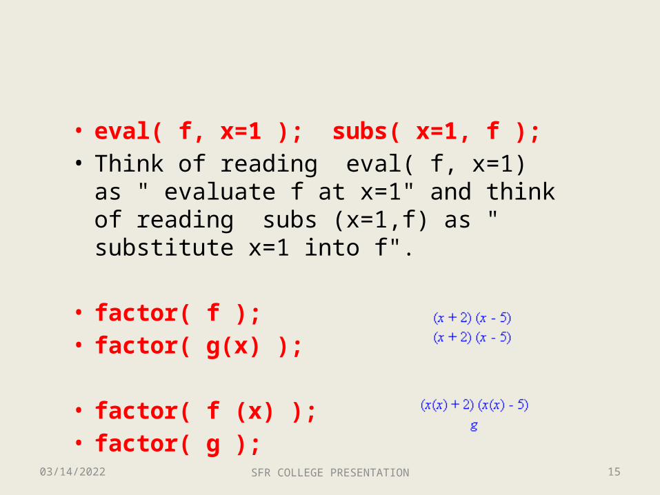
• eval( f, x=1 ); subs( x=1, f ); • Think of reading eval( f, x=1) as " evaluate f

at x=1" and think of reading subs (x=1,f) as " substitute x=1 into f".

• factor( f );• factor( g(x) );

• factor( f (x) );• factor( g );


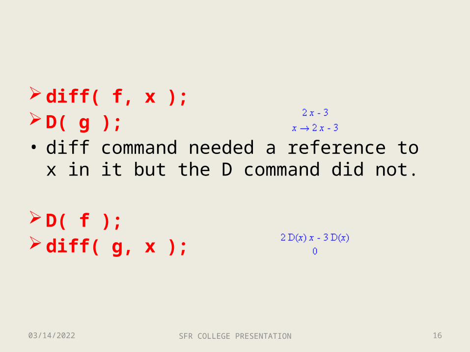
diff( f, x ); D( g );• diff command needed a reference to x in it but the D

command did not.

D( f ); diff( g, x );


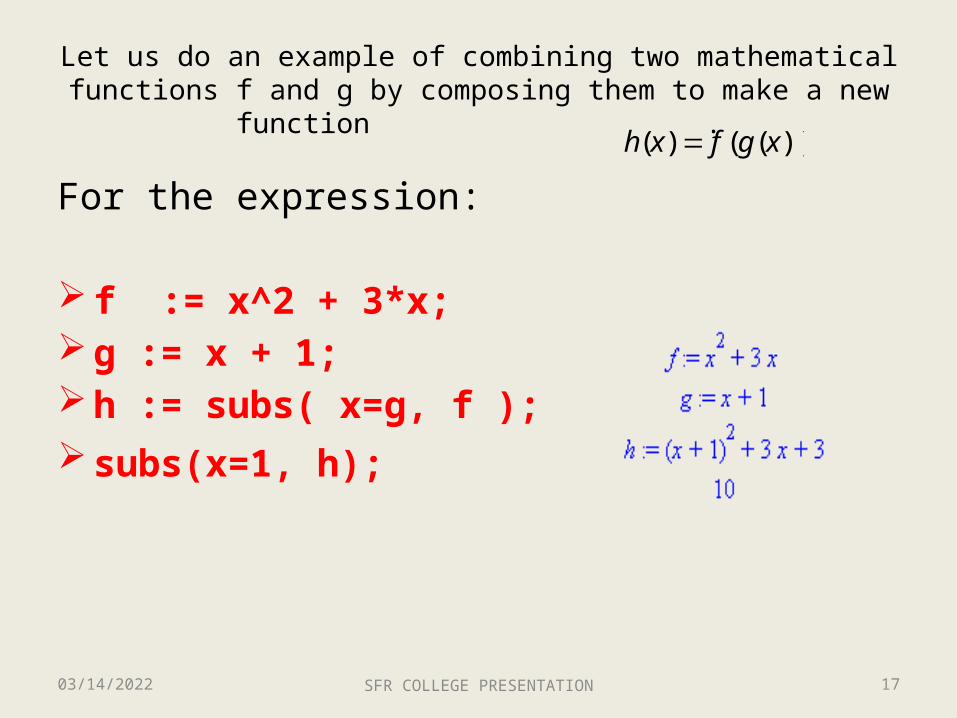
Let us do an example of combining two mathematical functions f and g by composing them to make a new function .

For the expression:

f := x^2 + 3*x; g := x + 1; h := subs( x=g, f ); subs(x=1, h);

))(()( xgfxh


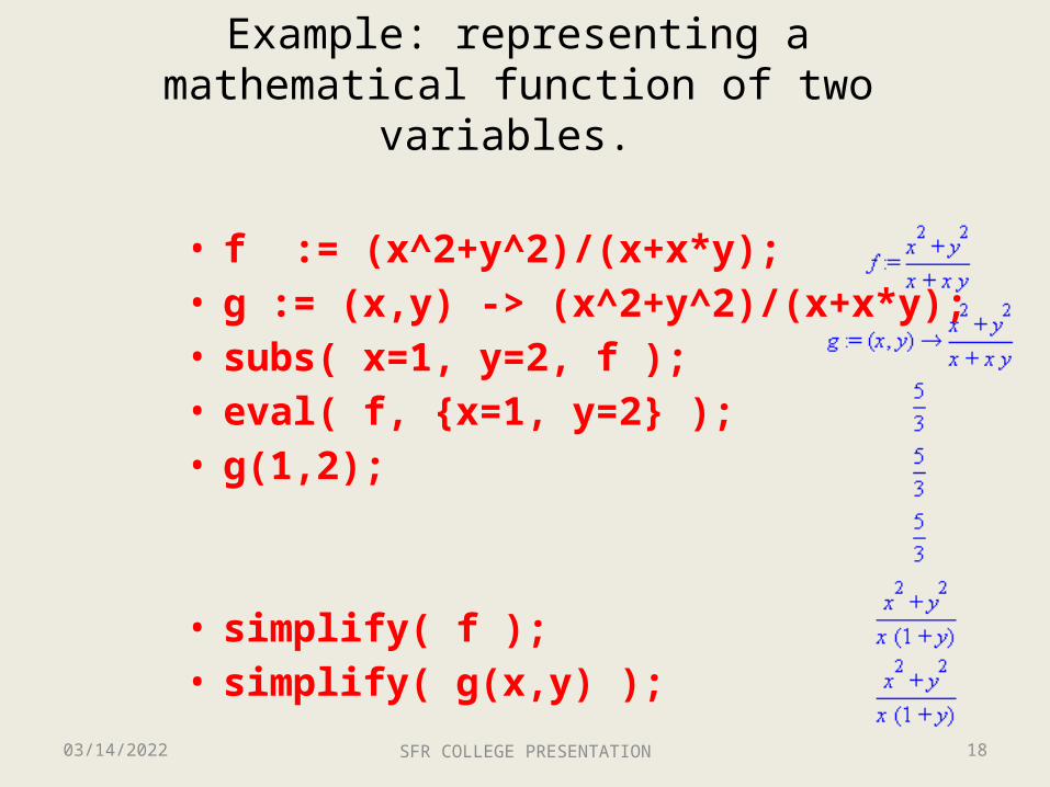
Example: representing a mathematical function of two variables.

• f := (x^2+y^2)/(x+x*y);• g := (x,y) -> (x^2+y^2)/(x+x*y);• subs( x=1, y=2, f );• eval( f, {x=1, y=2} );• g(1,2);

• simplify( f );• simplify( g(x,y) );


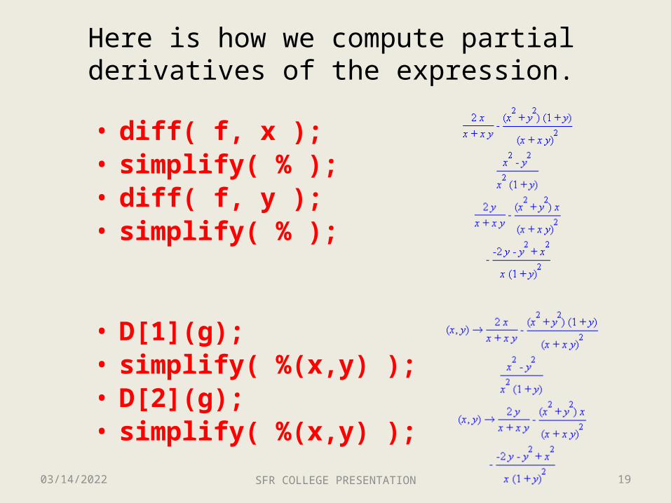
Here is how we compute partial derivatives of the expression.

• diff( f, x );• simplify( % );• diff( f, y );• simplify( % );

• D[1](g);• simplify( %(x,y) );• D[2](g);• simplify( %(x,y) );




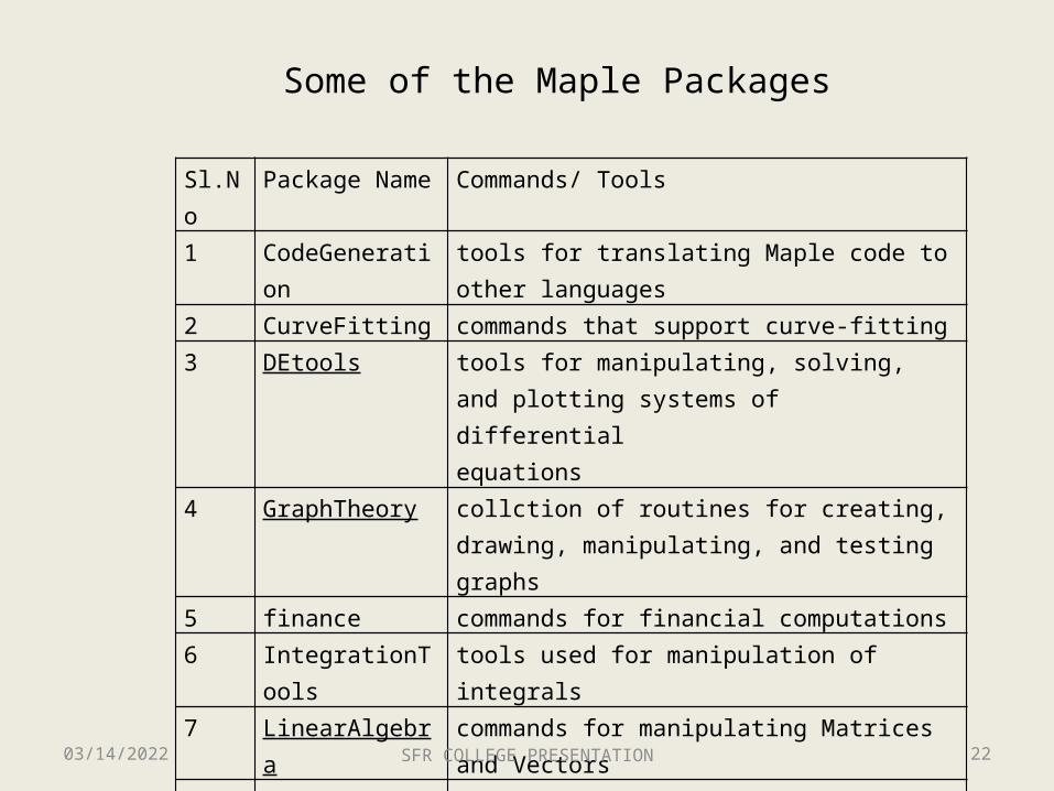
Sl.No Package Name Commands/ Tools

1 CodeGeneration tools for translating Maple code to other languages

2 CurveFitting commands that support curve-fitting

3 DEtools tools for manipulating, solving, and plotting systems of differential equations

4 GraphTheory collction of routines for creating, drawing, manipulating, and testing graphs

5 finance commands for financial computations

6 IntegrationTools tools used for manipulation of integrals

7 LinearAlgebra commands for manipulating Matrices and Vectors

8 IntegrationTools tools used for manipulation of integrals

9 numtheory commands for classic number theory

10 Optimization commands for numerically solving optimization theory problems

11 PDEtools tools for solving partial differential equations

12 Statistics tools for mathematical statistics and data analysis

Some of the Maple Packages


Differential Package

Graph Theory Package

Optimization Package

EXPLORING THE PACKAGES

Thank you for your

attention

Engineering

Mathematical Modeling With Maple