School of Electrical and Computer Engineering

Introduction to ElectronicsModule 1: Overview and Background

An introduction to electronic components and a study of circuits containing such devices.

Dr. Bonnie H. FerriProfessor and Associate ChairSchool of Electrical and Computer Engineering

School of Electrical and Computer Engineering

Review of Circuit Elements

Review linear circuit components and properties

Review Resistors, capacitors, inductors

i-v characteristics of these elements Sources, nodes

Lesson Objectives

3

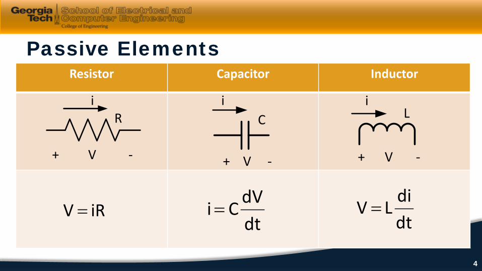
Passive ElementsResistor Capacitor Inductor

+ V -

iR

iRV =

+ V -

Ci

dtdVCi=

+ V -

Li

dtdiLV =

4

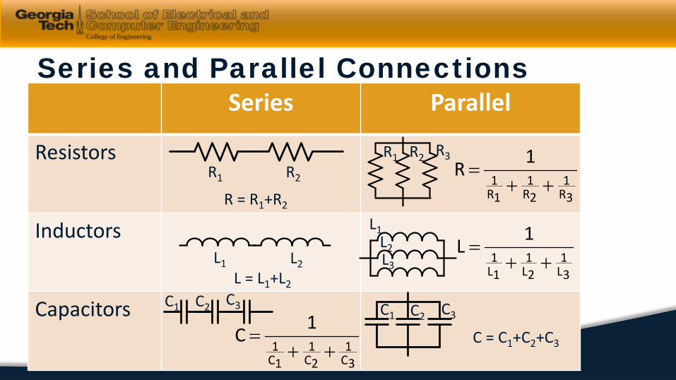
Series and Parallel ConnectionsSeries Parallel

Resistors

Inductors

Capacitors

R1 R2

R = R1+R2

R1 R2 R3

3R1

2R1

1R1

1R++

=

3C1

2C1

1C1

1C++

=

C1 C2 C3 C1 C2 C3

C = C1+C2+C3

3L1

2L1

1L1

1L++

=L = L1+L2

L1 L2

L1L2L3

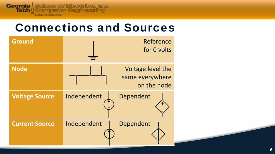
Connections and SourcesGround Reference

for 0 volts

Node Voltage level the same everywhere

on the node

Voltage Source Independent Dependent

Current Source Independent Dependent

+-

6

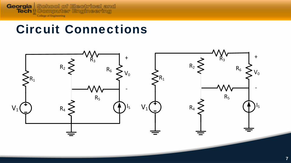
Circuit Connections

V1

R1

R2

R3

R4

R5

+

V0

-

R6

IS V1

R1

R2

R3

R4

R5

+

V0

-

R6

IS

7

Dr. Bonnie H. FerriProfessor and Associate ChairSchool of Electrical and Computer Engineering

School of Electrical and Computer Engineering

Review of Kirchoff’s Laws

Review of KVL and KCL

Review Kirchhoff’s Current Law (KCL) Kirchhoff’s Voltage Law (KVL)

Lesson Objectives

9

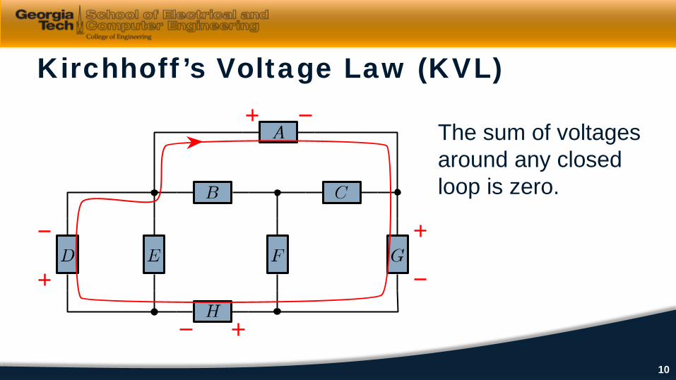
Kirchhoff’s Voltage Law (KVL)

The sum of voltages around any closed loop is zero.

10

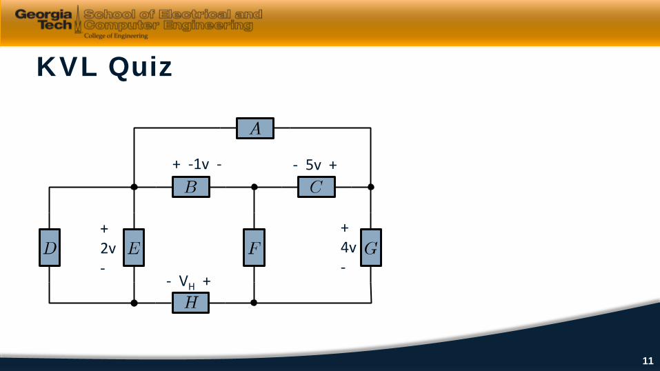
KVL Quiz

+2v-

+4v-

- 5v ++ -1v -

- VH +

11

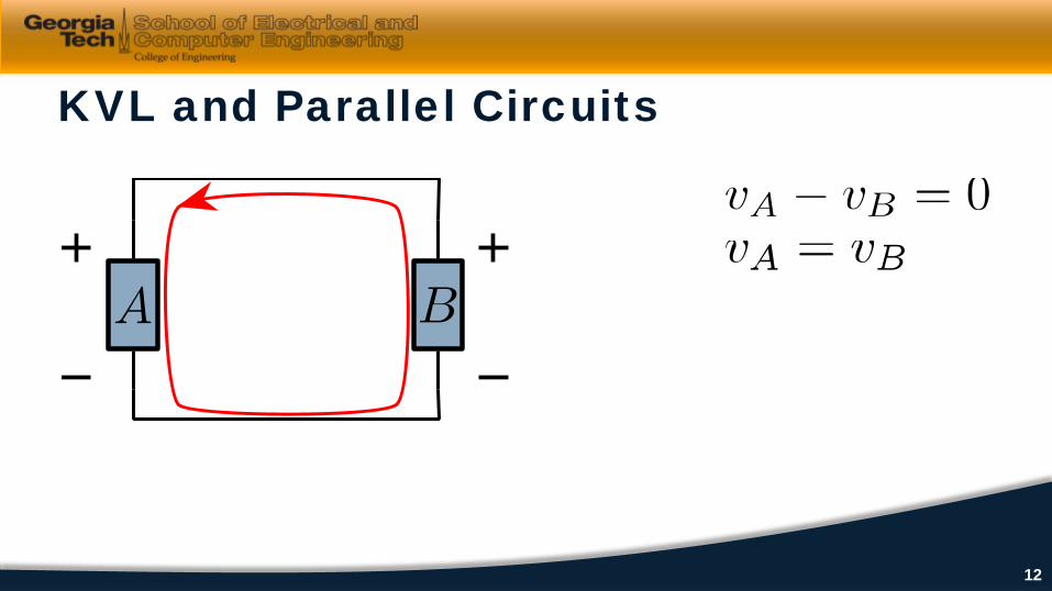
KVL and Parallel Circuits

12

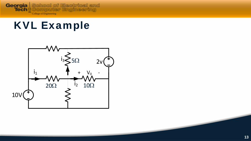
KVL Example

10V

2v

+ V0 -i1

i2

i3

20Ω 10Ω

5Ω

13

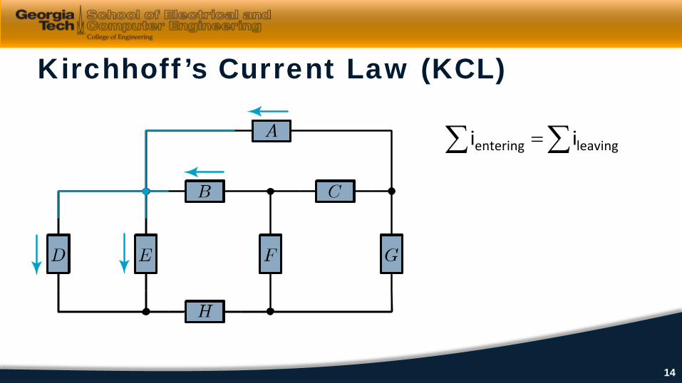
Kirchhoff’s Current Law (KCL)

∑ ∑= leavingentering ii

14

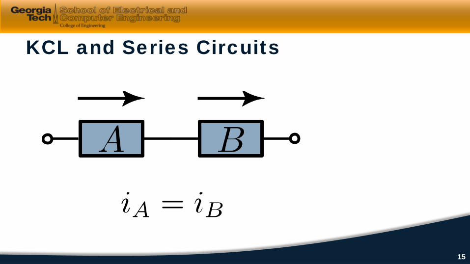
KCL and Series Circuits

15

KCL Example

10V

2v

+ V0 -i1

i2

i3

20Ω 10Ω

5Ω

16

Introduced KVL and KCL Applied KVL to parallel elements Applied KCL to series elements Solved a simple circuit using

Kirchhoff’s Laws

Summary

17

Dr. Bonnie H. FerriProfessor and Associate ChairSchool of Electrical and Computer Engineering

School of Electrical and Computer Engineering

Review of Impedance

Review of Impedance for Analyzing AC Circuits

Review Impedances for steady-state sinusoidal inputs (AC)

Lesson Objectives

19

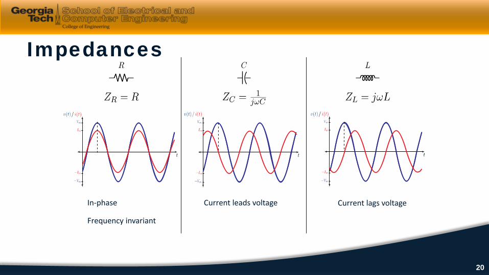
Impedances

In-phase Current leads voltage Current lags voltage

Frequency invariant

20

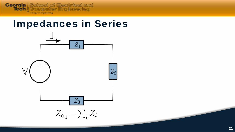
Impedances in Series

21

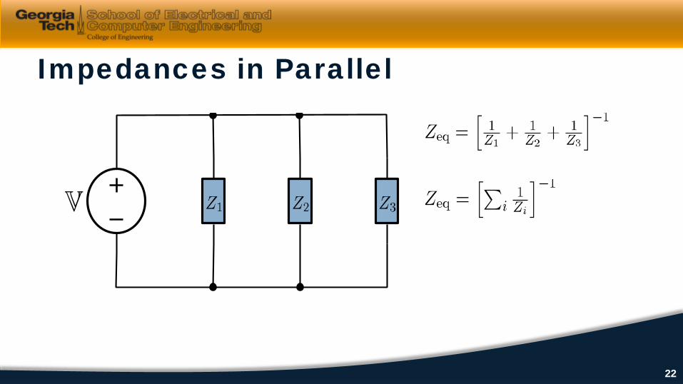
Impedances in Parallel

22

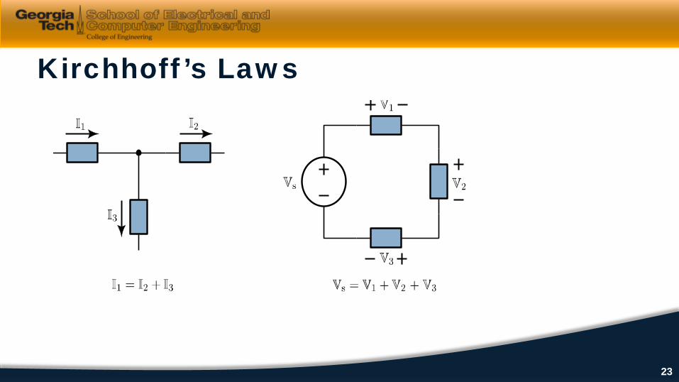
Kirchhoff’s Laws

23

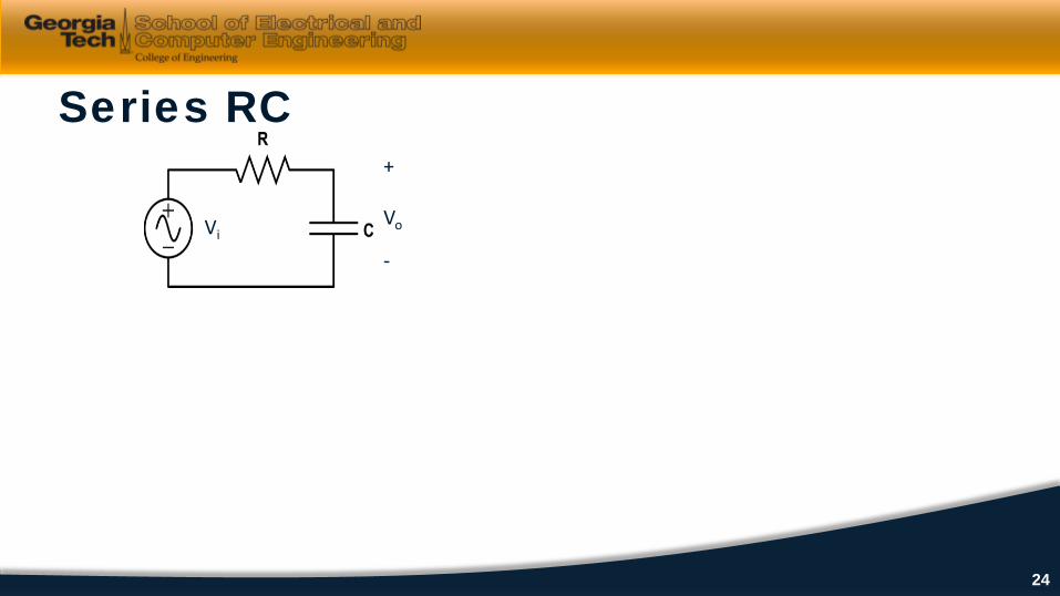
Series RC+

Vo

-Vi

24

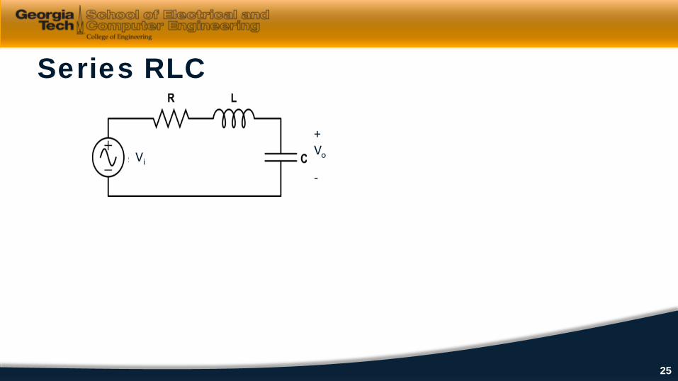
Series RLC

Vi

+Vo

-

25

Introduced KVL and KCL Applied KVL to parallel elements Applied KCL to series elements Solved a simple circuit using

Kirchhoff’s Laws

Summary

26

Dr. Bonnie H. FerriProfessor and Associate ChairSchool of Electrical and Computer Engineering

School of Electrical and Computer Engineering

Review of Transfer Functions

Review of transfer functions for characterizing circuits

Review transfer functions To characterize a circuit To find frequency response curves

Lesson Objectives

28

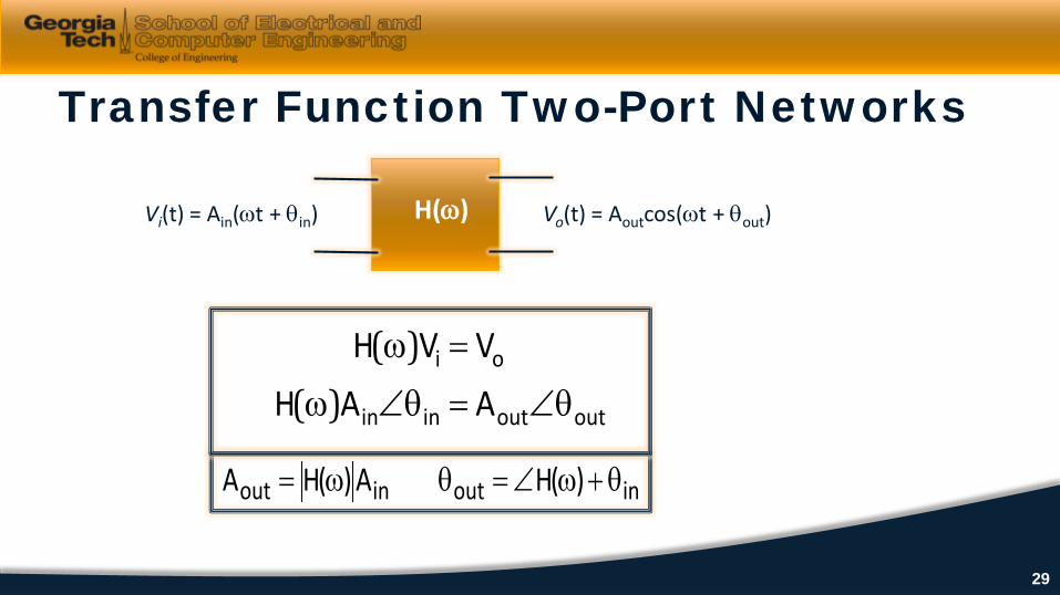
Transfer Function Two-Port Networks

Vi(t) = Ain(ωt + θin) H(ω) Vo(t) = Aoutcos(ωt + θout)

inoutinout )(HA)(HA θ+ω∠=θω=

outoutinin

oi

AAHVVH

θ∠=θ∠ω

=ω

)()(

29

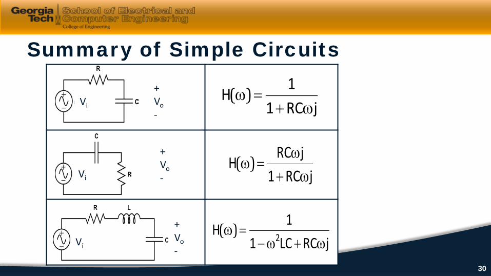
Summary of Simple Circuits

jRC11Hω+

=ω)(

+Vo-Vi

+Vo-

Vi

+Vo-

Vi jRCLC11H 2 ω+ω−

=ω)(

jRC1jRCHω+

ω=ω)(

30

Defined transfer function for Two-Port Networks Showed transfer functions of simple circuits

Summary

31

Dr. Bonnie H. FerriProfessor and Associate ChairSchool of Electrical and Computer Engineering

School of Electrical and Computer Engineering

Review of Frequency Response Plots (Bode)

Review of linear plots and Bode plots to show the frequency characteristics of signals and circuits

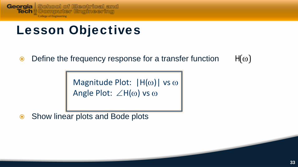
Define the frequency response for a transfer function

Show linear plots and Bode plots

Lesson Objectives

)(ωH

Magnitude Plot: |H(ω)| vs ωAngle Plot: ∠H(ω) vs ω

33

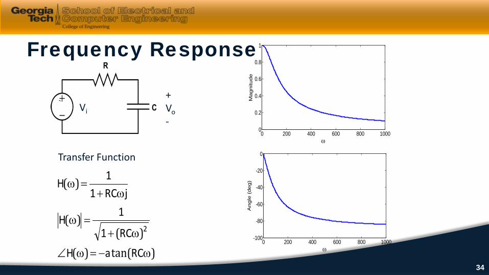
Frequency Response

0 200 400 600 800 10000

0.2

0.4

0.6

0.8

1

ω

Magnitu

de

0 200 400 600 800 1000-100

-80

-60

-40

-20

0

ωA

ngle

(deg)

Transfer Function

)tan()()(

)(

)(

ω−=ω∠

ω+=ω

ω+=ω

RCaHRC1

1H

jRC11H

2

+Vo-

Vi

34

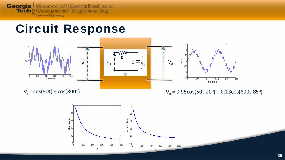
Circuit Response

Vi Vo

0 0.05 0.1 0.15 0.2 0.25-2

-1

0

1

2

Time (sec)

v(t)

0 0.05 0.1 0.15 0.2 0.25-1.5

-1

-0.5

0

0.5

1

1.5

Time (sec)

v(t)

0 200 400 600 800 10000

0.2

0.4

0.6

0.8

1

ω

Magnitude

Vi = cos(50t) + cos(800t) Vo = 0.95cos(50t-20o) + 0.13cos(800t-85o)

0 200 400 600 800 1000-100

-80

-60

-40

-20

0

ω

Angle

(deg)

35

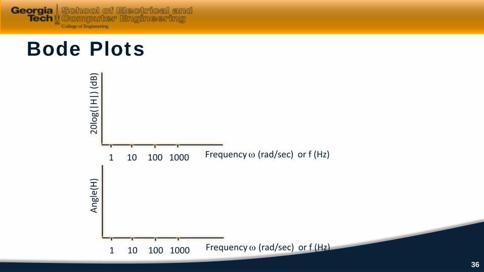
Bode Plots

Frequency ω (rad/sec) or f (Hz)1 10 100 1000

Frequency ω (rad/sec) or f (Hz)1 10 100 100036

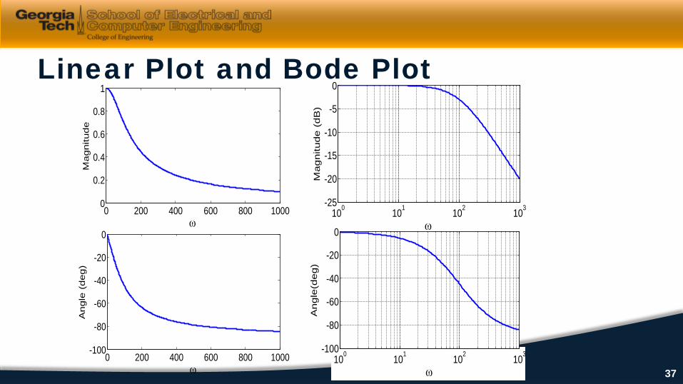
Linear Plot and Bode Plot

100 101 102 103-100

-80

-60

-40

-20

0

ω

Angle

(deg)

100 101 102 103-25

-20

-15

-10

-5

0

ω

Magnitu

de (

dB

)

0 200 400 600 800 1000-100

-80

-60

-40

-20

0

ω

Angle

(deg)

0 200 400 600 800 10000

0.2

0.4

0.6

0.8

1

ω

Magnitu

de

37

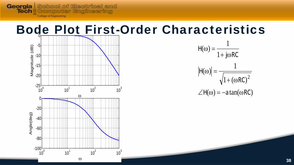
Bode Plot First-Order Characteristics

100 101 102 103-100

-80

-60

-40

-20

0

ω

Angle

(deg)

100 101 102 103-25

-20

-15

-10

-5

0

ω

Magnitu

de (

dB

)

)tan()()(1

1)(

11)(

2

RCaH

RCH

RCjH

ω−=ω∠

ω+=ω

ω+=ω

38

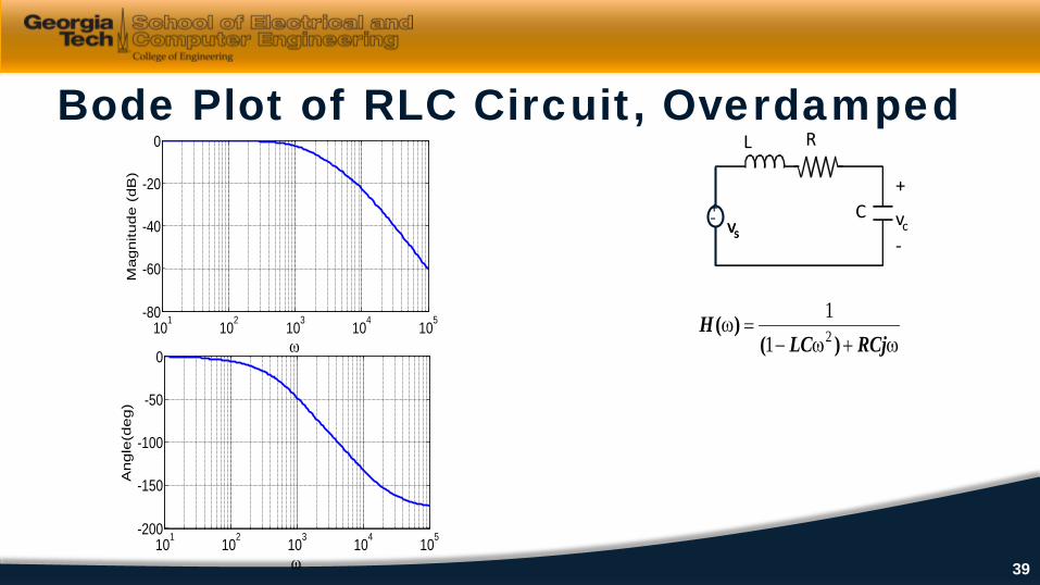
Bode Plot of RLC Circuit, Overdamped

101 102 103 104 105-80

-60

-40

-20

0

ω

Magnitu

de (

dB

)

101 102 103 104 105-200

-150

-100

-50

0

ω

Angle

(deg)

vs

+

-vc

C

L

vs

+-

-

R

ω+ω−=ω

RCjLCH

)()( 21

1

39

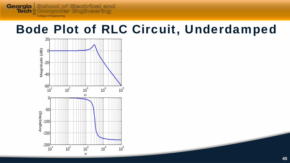
Bode Plot of RLC Circuit, Underdamped

101 102 103 104 105-60

-40

-20

0

20

ω

Magnitu

de (

dB

)

101 102 103 104 105-200

-150

-100

-50

0

ω

Angle

(deg)

40

A is a plot of the transfer function versus frequency

The frequency response can be used to determine the steady-state sinusoidal response of a circuit at different frequencies

Summary

41