Optical scanning holography with matlab ting chung poon

OPTICAL SCANNING HOLOGRAPHY WITH MATLAB®

OPTICAL SCANNING HOLOGRAPHYWITH MATLAB®

TING-CHUNG POON Bradley Department of Electrical and Computer Engineering, Virginia Tech, Blacksburg,Virginia 24061.

Dr. Ting-Chung Poon Virginia Tech Bradley Dept. Electrical and Computer Engineering Blacksburg, VA 24061 USA [email protected]

Library of Congress Control Number: 2007921127

ISBN-10: 0-387-36826-4 e-ISBN-10: 0-387-36826-4 ISBN-13: 978-0-387-36826-9 e-ISBN-13: 978-0-387-68851-0

Printed on acid-free paper.

© 2007 Springer Science+Business Media, LLC

9 8 7 6 5 4 3 2 1 springer.com

The use in this publication of trade names, trademarks, service marks and similar terms, even if they are not identified as such, is not to be taken as an expression of opinion as to whether or not they are subject to proprietary rights.

permission of the publisher (Springer Science+Business Media, LLC, 233 Spring Street, New York, All rights reserved. This work may not be translated or copied in whole or in part without the written

NY 10013, USA), except for brief excerpts in connection with reviews or scholarly analysis. Use in connection with any form of information storage and retrieval, electronic adaptation, computer software, or by similar or dissimilar methodology now know or hereafter developed is forbidden.

Dedication

This book is dedicated to

Eliza (M.S., Iowa 1980), Christina (B.S., Cornell 2004), and Justine (B.S., Virginia Tech 2007).

Contents

Preface ix

1 1

1.2 Linear and Invariant Systems . . . . . . . . . . . . . . . . . . . . . . . . . . . . . . 10

1.2.2 Convolution and Correlation Concept. . . . . . . . . . . . . . . . . . . 14

21 21 25

2.2.1 Plane Wave Solution . . . . . . . . . . . . . . . . . . . . . . . . . . . . . . . 25 2.2.2 Spherical Wave Solution . . . . . . . . . . . . . . . . . . . . . . . . . . . . 27

29 2.3.1 Fresnel Diffraction . . . . . . . . . . . . . . . . . . . . . . . . . . . . . . . . . 33

2.4 Ideal Lens, Imaging Systems, Pupil Functions

40 43 45 49 49

2.3 Scalar Diffraction Theory . . . . . . . . . . . . . . . . . . . . . . . . . . . . . . . .

2.2 Three-Dimensional Scalar Wave Equation . . . . . . . . . . . . . . . . . . .

1. Mathematical Background and Linear System. . . . . . . . . . . . . . . . . . . . . . . . . . . 1.1 Fourier Transformation . . . . . . . . . . . . . . . . . . . . . . . . . . . . . . . . . . . . . . . . .

. . . . . .

1.2.1 Linearity and Invariance . . . . . . . . . . . . . . . . . . . . . . . . . . . . . . . . . . . 1 0 . . . . . .

. . . . . .2. Wave Optics and Holography . . . . . . . . . . . . . . . . . . . . . . . . . . . . . . . . .

. . . . . . . . . . . . . . . . . . . . . . . . . . . . . . 2.3.2 Diffraction of a Square Aperture. . . . . . . . . . . . . . . . . . . . . . . . . . . . . 36

2.5.3 Digital Holography . . . . . . . . . . . . . . . . . . . . . . . . . . . . . . . . . . . . . . . 60 2.5.2 Off-Axis Holography . . . . . . . . . . . . . . . . . . . . . . . . . . . . . . . . . . . . . 57 2.5.1 Fresnel Zone Plate as a Point-Source Hologram . . . . . . . . . . . . . . . . 2.5 Holography . . . . . . . . . . . . . . . . . . . . . . . . . . . . . . . . . . . . . . . . . . . . . . . . . . 2.4.3 Incoherent Image Processing . . . . . . . . . . . . . . . . . . . . . . . . . . . . . . . 2.4.2 Coherent Image Processing . . . . . . . . . . . . . . . . . . . . . . . . . . . . . . . . 2.4.1 Ideal Lens and Optical Fourier Transformation . . . . . . . . . . . . . . . . .

and Transfer Functions. . . . . . . . . . . . . . . . . . . . . . . . . . . . . . . . . . . . . . . . 40

2.1 Maxwell’s Equations and Homogeneous Vector Wave Equation . . . . . . . .

65

72 75 81 92

97 97

141 143

149

viii Optical Scanning Holography with MATLAB

3.1 Principle of Optical Scanning . . . . . . . . . . . . . . . . . . . . . . . . . . . . . . . . . . . 3. Optical Scanning Holography: Principles . . . . . . . . . . . . . . . . . . . . . . . . . . . . . . 65

3.2 Optical Heterodyning. . . . . . . . . . . . . . . . . . . . . . . . . . . . . . . . . . . . . . . . . 69 3.3 Acousto-Optic Frequency Shifting . . . . . . . . . . . . . . . . . . . . . . . . . . . . . . . 3.4 Two-Pupil Optical Heterodyne Scanning Image Processor . . . . . . . . . . . . 3.5 Scanning Holography . . . . . . . . . . . . . . . . . . . . . . . . . . . . . . . . . . . . . . . . . 3.6 Physical Intuition to Optical Scanning Holography . . . . . . . . . . . . . . . . . .

4. Optical Scanning Holography: Applications . . . . . . . . . . . . . . . . . . . . . . . . . . . . 4.1 Scanning Holographic Microscopy . . . . . . . . . . . . . . . . . . . . . . . . . . . . . . .

4.3 Optical Scanning Cryptography . . . . . . . . . . . . . . . . . . . . . . . . . . . . . . . . . 117

5.3 PSF Engineering . . . . . . . . . . . . . . . . . . . . . . . . . . . . . . . . . . . . . . . . . . . . . 5.2 Single-Beam Scanning vs. Double-Beam Scanning . . . . . . . . . . . . . . . . . . 5.1 Coherent and Incoherent Holographic Processing . . . . . . . . . . . . . . . . . . . 1355. Optical Scanning Holography: Advances . . . . . . . . . . . . . . . . . . . . . . . . . . . . . . 135

Index . . . . . . . . . . . . . . . . . . . . . . . . . . . . . . . . . . . . . . . . . . . . . . . . . . . . . . . . . . . . .

4.2 Three-Dimensional Holographic TV and 3-D Display . . . . . . . . . . . . . . . . 106

Preface

This book serves two purposes. The first is to succinctly cover the necessary mathematical background and wave optics that pertain to Fourier optics and holography. The second is to introduce optical scanning holography (OSH) - a form of electronic (or digital) holography - to the readers, and to provide them with experience in modeling the theory and applications utilizing MATLAB®. Optical Scanning Holography with MATLAB® consists of tutorials (with numerous MATLAB examples throughout the text), research material, as well as new ideas and insights that are useful for engineering or physics students, scientists, and engineers working in the fields of Fourier optics, optical scanning imaging and holography. The book is self-contained and covers the basic principles of OSH. Thus, this book will be relevant for years to come. The writing style of this book is geared towards undergraduate seniors or first-year graduate-level students in the fields of engineering and physics. The material covered in this book is suitable for a one-semester course in Fourier optics, optical scanning imaging and holography. Optical scanning holography is a highly sophisticated technology that consists of numerous facets and applications. It is a real-time (or on-the-fly) holographic recording technique that is based on active optical heterodyne scanning. It is a relatively new area in electronic holography and will potentially lead science and technology to many novel applications such as cryptography, 3-D display, scanning holographic microscopy, 3-D pattern recognition and 3-D optical remote sensing. The main purpose of this book is to introduce optical scanning holography to the readers in a manner that will allow them to feel comfortable enough to explore the technology on

x

their own - possibly even encourage them to begin implementing their own set-ups in order to create novel OSH applications. Optical scanning holography is generally a simple yet powerful technique for 3-D imaging, and it is my aspiration that this book will stimulate further research of optical scanning holography and its various novel applications. I have incorporated some of the material from this book into my short course entitled Optical Scanning Holography at SPIE Photonics West, in lectures given at the Institute of Optical Sciences (IOS), which is now known as the Department of Optics and Photonics, National Central University (NCU), Taiwan, and also at the Department of Electronics and Computer Science, Nihon University, Japan. The book was finally completed during my time as a visiting professor at Nihon University. I want to take this opportunity to thank my host, Professor Hiroshi Yoshikawa, for his hospitality and arranging a spacious office for me that allowed me to concentrate on the last phase of this book. I would also like to thank Professor Hon-Fai Yau of NCU for providing me with some early opportunities (when the book was still in its infancy) to “rehearse” my optical scanning holography lectures at IOS. I would like to thank my wife, Eliza, and my children, Christina and Justine, for their encouragement, patience, and love. This book is dedicated to them. In addition, I would also like to thank Christina Poon for reading the manuscript and providing comments and suggestions for improvement.

“ ”

Optical Scannning Holography with MATLAB

Chapter 1

Mathematical Background andLinear Systems

1.1 Fourier Transformation

In electrical engineering, we are most concerned with a signal as a functionof time, . The signal in question could be a voltage or a current. The0Ð>Ñforward temporal Fourier transform of is given as0Ð>Ñ

Y Ö0Ð>Ñ× œ JÐ Ñ œ 0Ð>Ñ Ð 4 >Ñ .>= =(_

_

exp , (1.1-1a)

where the transform variables are time, [second], and temporal radian>

frequency, [radian/second]. In Eq. (1.1a), . The inverse Fourier= 4 œ "Ètransform is

Y "ÖJ Ð Ñ× œ 0Ð>Ñ œ JÐ Ñ Ð4 >Ñ ."

#= = = =

1(_

_

exp . (1.1-1b)

In optics, we are most interested in dealing with a two-dimensional (2-D)

.Hence, the two-dimensional spatial of a signal isFourier transform 0ÐBß CÑgiven as [Banerjee and Poon (1991), Poon and Banerjee (2001)]

YBCÖ0ÐBß CÑ× œ JÐ5 5 Ñ œ 0ÐBß CÑ Ð45 B 45 CÑ .B.CB C B C_ _

_ _

, exp ,( ((1.1-2a)

and the inverse Fourier transform is

, YBC"ÖJ Ð5 5 Ñ×B C

œ 0ÐBß CÑ

, exp , (1.1-2b)œ JÐ5 5 Ñ Ð 45 B 45 CÑ .5 .5"

%1#_ _

_ _

B C B C B C( (where the transform variables are spatial variables, [meter], and spatialBß Cradian frequencies, , [radian/meter]. and , are a Fourier5 5 ÐBß CÑ J Ð5 5 ÑB C B C0

signal. Examples include images or the transverse profile of an electro-magnetic or optical field at some plane of spatial variables B C and

transform pair and the statement is symbolically represented by

,0ÐBß CÑ Í JÐ5 5 ÑÞB C

Note that the definitions for the forward and inverse transforms [see Eqs.(1.1-2a) and (1.1-2b)] are consistent with the engineering convention for atraveling wave, as explained in [Banerjee andPrinciples of Applied Optics Poon (1991)]. Common properties and examples of 2-D Fourier transformappear in the Table below.

Table 1.1 Properties and examples of some two-dimensional Fourier Transforms. Function in Fourier transform in ( )ÐBß CÑ 5 ß 5B C

. ,1 0ÐBß CÑ J Ð5 5 ÑB C

. , exp2 0ÐB B ß C C Ñ J Ð5 5 Ñ Ð45 B 45 C Ñ! ! B C B ! C !

complex constants ,3Þ 0 Ð+Bß ,CÑà +ß , J Ð Ñ"+,

5+ ,

5¸ ¸ B C

. ,4 0 ÐBß CÑ J Ð 5 5 Ñ‡ ‡B C

/ ,5Þ `0ÐBß CÑ `B 45 JÐ5 5 ÑB B C

. / ,6 ` 0ÐBß CÑ `B`C 5 5 JÐ5 5 Ñ#B C B C

. 7 delta function $ÐBß CÑ œ / .5 .5 ""

% _ __ _ „45 B„45 C

B C1#B C' '

. 1 ,8 % Ð5 5 Ñ1 $# B C

. 9 rectangle function sinc function rect rect rect , sinc sinc sinc ,ÐBß CÑ œ ÐBÑ ÐCÑ Ð ß Ñ œ Ð Ñ Ð Ñ5 5

# # # #

5 5B BC C

1 1 1 1

where rect where sincÐBÑ œ ÐBÑ œŠ ‹"ß B "Î#!ß

Ð BÑB

otherwise

sin¸ ¸ 11

. 10 Gaussian function Gaussian function exp ] expÒ ÐB C Ñ Ò Ó! # # 5 5

%1! !

B C# #

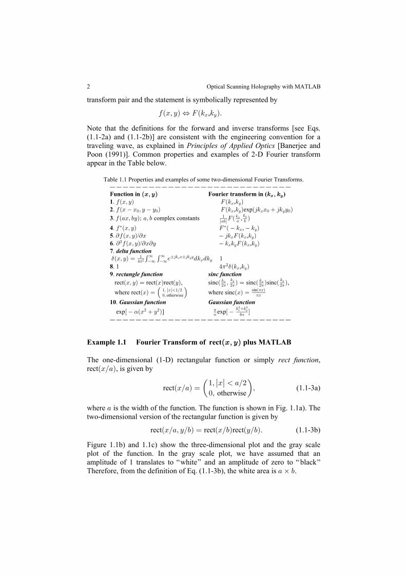
Example 1.1 Fourier Transform of rect plus MATLAB ÐBß CÑ

The one-dimensional (1-D) rectangular function or simply ,rect functionrect , is given byÐBÎ+Ñ

rect (1.1-3a)otherwise

ÐBÎ+Ñ œ ß"ß B +Î#

!ßŒ ¸ ¸

where is the width of the function. The function is shown in Fig. 1.1a). The+two-dimensional version of the rectangular function is given by

rect rect rect . (1.1-3b)ÐBÎ+ß CÎ,Ñ œ ÐBÎ,Ñ ÐCÎ,Ñ

Figure 1.1b) and 1.1c) show the three-dimensional plot and the gray scaleplot of the function. In the gray scale plot, we have assumed that anamplitude of 1 translates to white and an amplitude of zero to blackTherefore, from the definition of Eq. (1.1-3b), the white area is .+ ‚ ,

2

“ ” “ ”

Optical Scanning Holography with MATLAB

3

Fig. 1.1 Rect function.

To find the Fourier transform of the 2-D rectangular function, we simplyevaluate the integral given by Eq. (1.1-2a) by recognizing that 0ÐBß CÑ œrect . Therefore, we writeÐBÎ+ß CÎ,Ñ

Y YBC BCÖ0 ÖÐBß CÑ× œ ÐBÎ+ß CÎ,Ñ×rect

œ ÐBÎ+ß CÎ,Ñ Ð45 B 45 CÑ.B.C( (_ _

_ _

B Crect exp . (1.1-4)

Since rect is a [see Eq. 1.1-3b)], we re-writeÐBÎ+ß CÎ,Ñ separable function Eq. (1.1-4) as follows:

YBCÖrectÐBÎ+ß CÎ,Ñ×

œ ÐBÎ+Ñ Ð45 BÑ.B ‚ ÐCÎ,Ñ Ð45 CÑ.C( (_ _

_ _

B Crect exp rect exp

exp exp . (1.1-5)œ " Ð45 BÑ.B ‚ " Ð45 CÑ.C( (+Î# ,Î#

+Î# ,Î#

B C

Mathematical Background and Linear Systems

4

By writing the last step, Eq. (1.1-5), we have used the definition of therectangular function given by Eq. (1.1-3a). We can now evaluate Eq. (1.1-5)by using

exp exp . (1.1-6)( Ð-BÑ.B œ Ð-BÑ"

-

Therefore,

exp sinc , (1.1-7)(+Î#

+Î#

BB

" Ð45 BÑ.B œ + Ð Ñ+5

#1

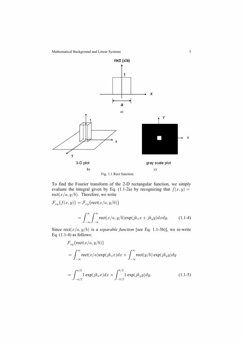
where is defined as the . Table 1.2 shows thesincÐBÑ œ sinÐ BÑ11B sinc function

m-file for plotting the sinc function and its output is shown in Fig. 1.2. Notethat the sinc function has zeros at ...B œ „ "ß „ #ß „ $ß

Table 1.2 Plot_sinc.m: m-file for plotting the sinc function.-----------------------------------------------------%Plot_sinc.m Plotting of sinc(x) functionx= -5.5:0.01:5.5;sinc=sin(pi*x)./(pi*x);plot(x,sinc)axis([-5.5 5.5 -0.3 1.1])grid onxlabel('x')ylabel('sinc (x)')------------------------------------------------------

Fig. 1.2 Sinc function.

To complete the original problem of determining the Fourier transform of arect function, we take advantage of the result of Eq. (1.1-7); Eq. (1.1-5)

−5 −4 −3 −2 −1 0 1 2 3 4 5

−0.2

0

0.2

0.4

0.6

0.8

1

x

sinc

(x)


5

becomes

rect sinc sincYBCÖ ÐBÎ+ß CÎ,Ñ× œ +, Ð Ñ Ð Ñ+5

# #

,5B C

1 1

œ +, Ð ß Ñ+5

# #

,5 sinc . (1.1-8a)B C

1 1Hence, we may write

rect sinc . (1.1-8b)ÐBÎ+ß CÎ,Ñ Í +, Ð ß Ñ+5

# #

,5B C

1 1

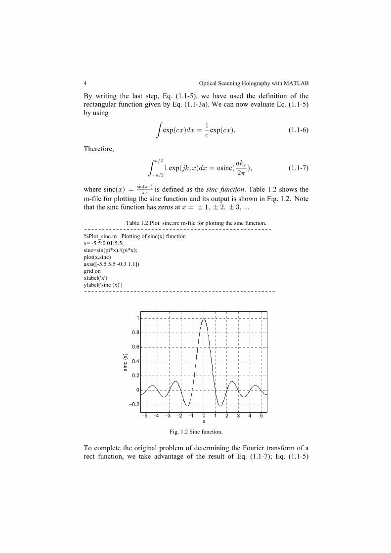
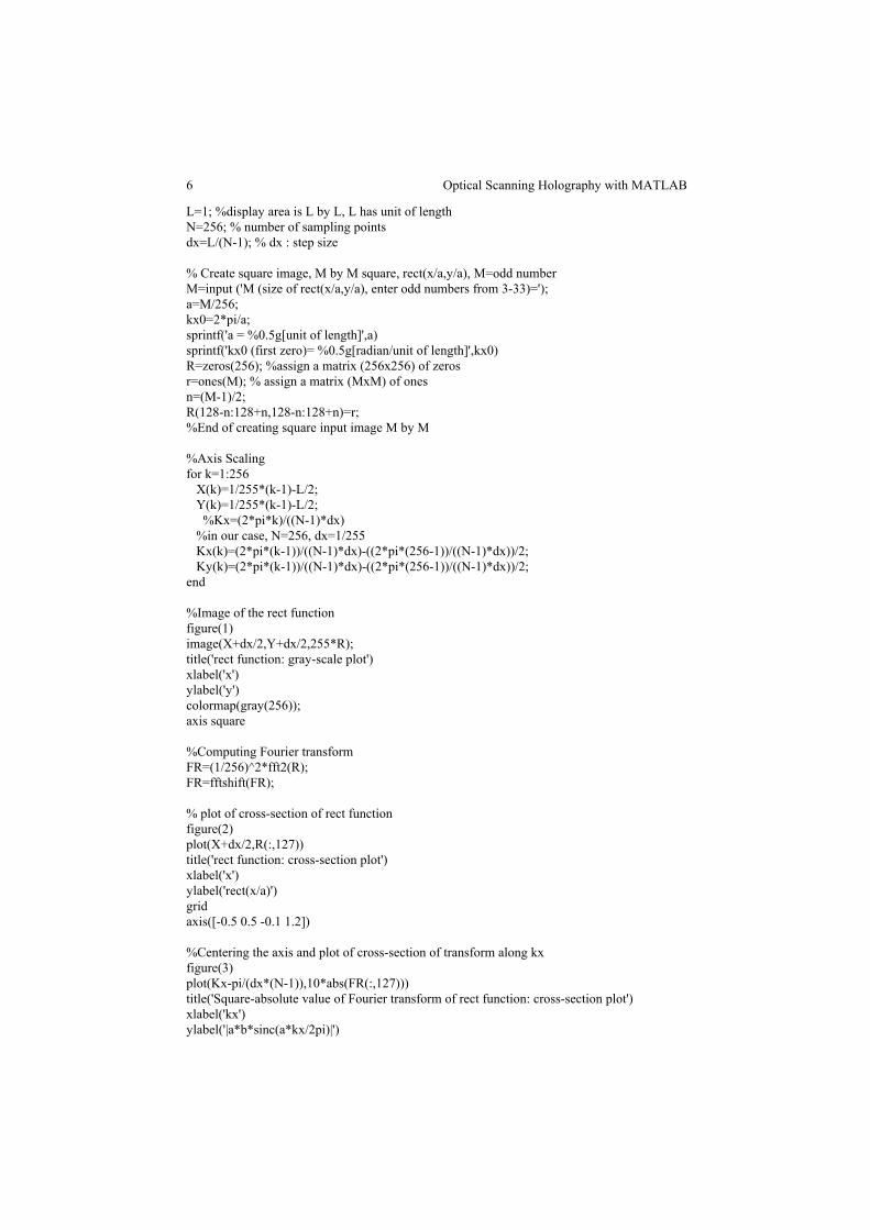
Note that when the width of the rect function along is , the first zero alongB +5 5 œ # Î+ÞB Bß! is Figure 1.3 shows the transform pair of Eq. (1.1-8b). The1top figures are 2-D gray-scale plots, and the bottom figures are line tracesalong the horizontal axis through the center of the top figures. These figuresare generated using the m-file shown in Table 1.3 where M 11. For thisœvalue of M, units of length and the first zero + œ !Þ!%#* 5 œ "%'Þ#$Bß!

radian/ unit of length . Note that the area of display in the - plane has beenÐ Ñ B Cscaled to 1 unit of length by 1 unit of length.

Fig. 1.3 Rect function and its Fourier transform.

Table 1.3 fft2Drect.m: m-file for 2-D Fourier transform of rect . ÐBÎ+ß CÎ,Ñ------------------------------------------------------%fft2Drect.m %Simulation of Fourier transformation of a 2-D rect function%clear


6

L=1; %display area is L by L, L has unit of lengthN=256; % number of sampling pointsdx=L/(N-1); % dx : step size

% Create square image, M by M square, rect(x/a,y/a), M=odd numberM=input ('M (size of rect(x/a,y/a), enter odd numbers from 3-33)=');a=M/256;kx0=2*pi/a;sprintf('a = %0.5g[unit of length]',a)sprintf('kx0 (first zero)= %0.5g[radian/unit of length]',kx0)R=zeros(256); %assign a matrix (256x256) of zerosr=ones(M); % assign a matrix (MxM) of onesn=(M-1)/2;R(128-n:128+n,128-n:128+n)=r;%End of creating square input image M by M

%Axis Scalingfor k=1:256 X(k)=1/255*(k-1)-L/2; Y(k)=1/255*(k-1)-L/2; %Kx=(2*pi*k)/((N-1)*dx) %in our case, N=256, dx=1/255 Kx(k)=(2*pi*(k-1))/((N-1)*dx)-((2*pi*(256-1))/((N-1)*dx))/2; Ky(k)=(2*pi*(k-1))/((N-1)*dx)-((2*pi*(256-1))/((N-1)*dx))/2;end

%Image of the rect functionfigure(1)image(X+dx/2,Y+dx/2,255*R);title('rect function: gray-scale plot')xlabel('x')ylabel('y')colormap(gray(256));axis square

%Computing Fourier transformFR=(1/256)^2*fft2(R);FR=fftshift(FR);

% plot of cross-section of rect functionfigure(2)plot(X+dx/2,R(:,127))title('rect function: cross-section plot')xlabel('x')ylabel('rect(x/a)')gridaxis([-0.5 0.5 -0.1 1.2])

%Centering the axis and plot of cross-section of transform along kxfigure(3)plot(Kx-pi/(dx*(N-1)),10*abs(FR(:,127)))title('Square-absolute value of Fourier transform of rect function: cross-section plot')xlabel('kx')ylabel('|a*b*sinc(a*kx/2pi)|')


7

axis([-800 800 0 max(max(abs(FR)))*10.1])grid

%Mesh the Fourier transformationfigure(4);mesh(Kx,Ky,(abs(FR)).^2)title('Square-absolute value of Fourier transform of rect function: 3-D plot,scalearbitrary')xlabel('kx')ylabel('ky')axis square

%Image of the Fourier transformation of rectangular functionfigure(5);gain=10000;image(Kx,Ky,gain*(abs(FR)).^2/max(max(abs(FR))).^2)title('Square-absolute value of Fourier transform of the rect function: gray-scale plot')xlabel('kx')ylabel('ky')axis squarecolormap(gray(256))------------------------------------------------------

Example 1.2 MATLAB Example:Fourier Transform of Bitmap Images

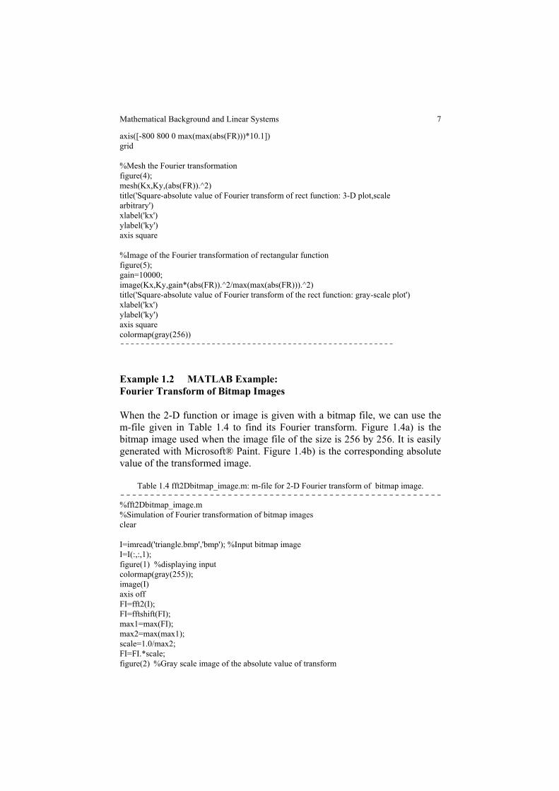
When the 2-D function or image is given with a bitmap file, we can use them-file given in Table 1.4 to find its Fourier transform. Figure 1.4a) is thebitmap image used when the image file of the size is 256 by 256. It is easilygenerated with Microsoft® Paint. Figure 1.4b) is the corresponding absolutevalue of the transformed image.

Table 1.4 fft2Dbitmap_image.m: m-file for 2-D Fourier transform of bitmap image.------------------------------------------------------%fft2Dbitmap_image.m%Simulation of Fourier transformation of bitmap imagesclear

I=imread('triangle.bmp','bmp'); %Input bitmap imageI=I(:,:,1);figure(1) %displaying inputcolormap(gray(255));image(I)axis offFI=fft2(I);FI=fftshift(FI);max1=max(FI);max2=max(max1);scale=1.0/max2;FI=FI.*scale;figure(2) %Gray scale image of the absolute value of transform


8

colormap(gray(255));image(10*(abs(256*FI)));axis off------------------------------------------------------

Fig. 1.4 Bitmap image and its transform generated using the m-file in Table 1.4.

Example 1.3 Delta Function and its Transform

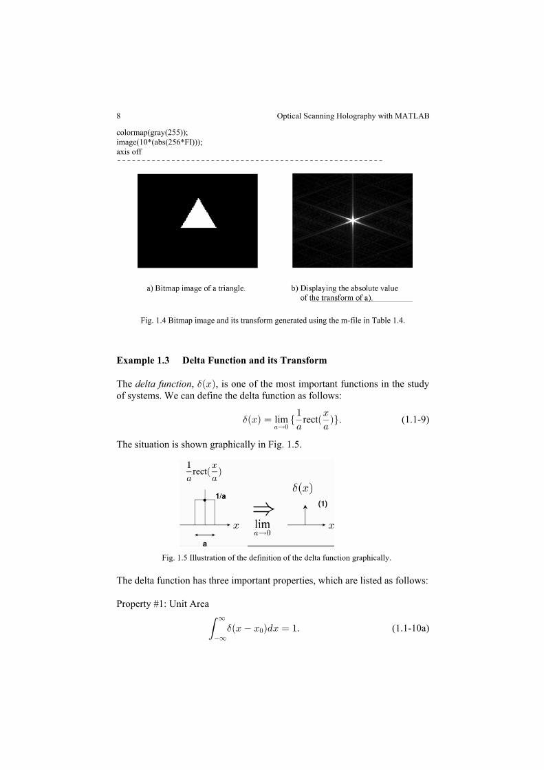
The , , is one of the most important functions in the studydelta function $ÐBÑof systems. We can define the delta function as follows:

$ÐBÑ œ Ö Ð Ñ×" B

+ +lim+Ä!

rect . (1.1-9)

The situation is shown graphically in Fig. 1.5.

Fig. 1.5 Illustration of the definition of the delta function graphically.

The delta function has three important properties, which are listed as follows:

Property #1: Unit Area

(_

_

!$ÐB B Ñ.B œ ". (1.1-10a)


9

The delta function has a unit area (or strength), which is denoted by a (1)beside the arrow, as shown in Fig. 1.5. This unit area property is clearlydemonstrated by the definition illustrated on the left hand side of Fig. 1.5.The area is always a unity regardless of the value of .+

Property #2: Product Property

0ÐBÑ ÐB B Ñ œ 0ÐB Ñ ÐB B Ñ$ $! ! ! . (1.1-10b)

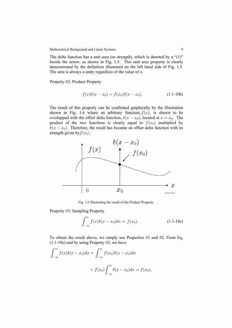
The result of this property can be confirmed graphically by the illustrationshown in Fig. 1.6 where an arbitrary function, , is shown to be0ÐBÑoverlapped with the offset delta function, , located at . The$ÐB B Ñ B œ B! !

product of the two functions is clearly equal to multiplied by0ÐB Ñ!$ÐB B ÑÞ! Therefore, the result has become an offset delta function with itsstrength given by .0ÐB Ñ!

Fig. 1.6 Illustrating the result of the Product Property.

Property #3: Sampling Property

. (1.1-10c)(_

_

! !0ÐBÑ ÐB B Ñ.B œ 0ÐB Ñ$

To obtain the result above, we simply use Properties #1 and #2. From Eq.(1.1-10c) and by using Property #2, we have

( (_ _

_ _

! ! !0ÐBÑ ÐB B Ñ.B œ 0ÐB Ñ ÐB B Ñ.B$ $

,œ 0ÐB Ñ ÐB B Ñ.B œ 0ÐB Ñ! ! !_

_( $

“ ”


10

where we have used Property #1 to obtain the last step of the result. Equation(1.1-10c) is known as the because the delta functionsampling propertyselects, or samples, a particular value of the function, , at the location of0ÐBÑthe delta function (i.e., ) in the integration process.B!

While a 1-D delta function is called an impulse function in electrical

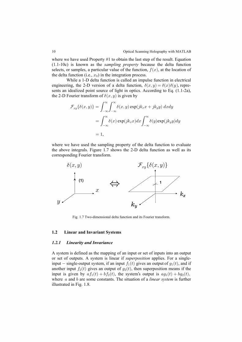
YBCÖ$ $ÐBß CÑ× œ ÐBß CÑ Ð45 B 45 CÑ .B.C( (_ _

_ _

B Cexp

exp expœ ÐBÑ Ð45 BÑ.B ÐCÑ Ð45 CÑ.C( (_ _

_ _

B C$ $

,œ "

where we have used the sampling property of the delta function to evaluatethe above integrals. Figure 1.7 shows the 2-D delta function as well as itscorresponding Fourier transform.

Fig. 1.7 Two-dimensional delta function and its Fourier transform.

1.2 Linear and Invariant Systems

1.2.1 Linearity and Invariance

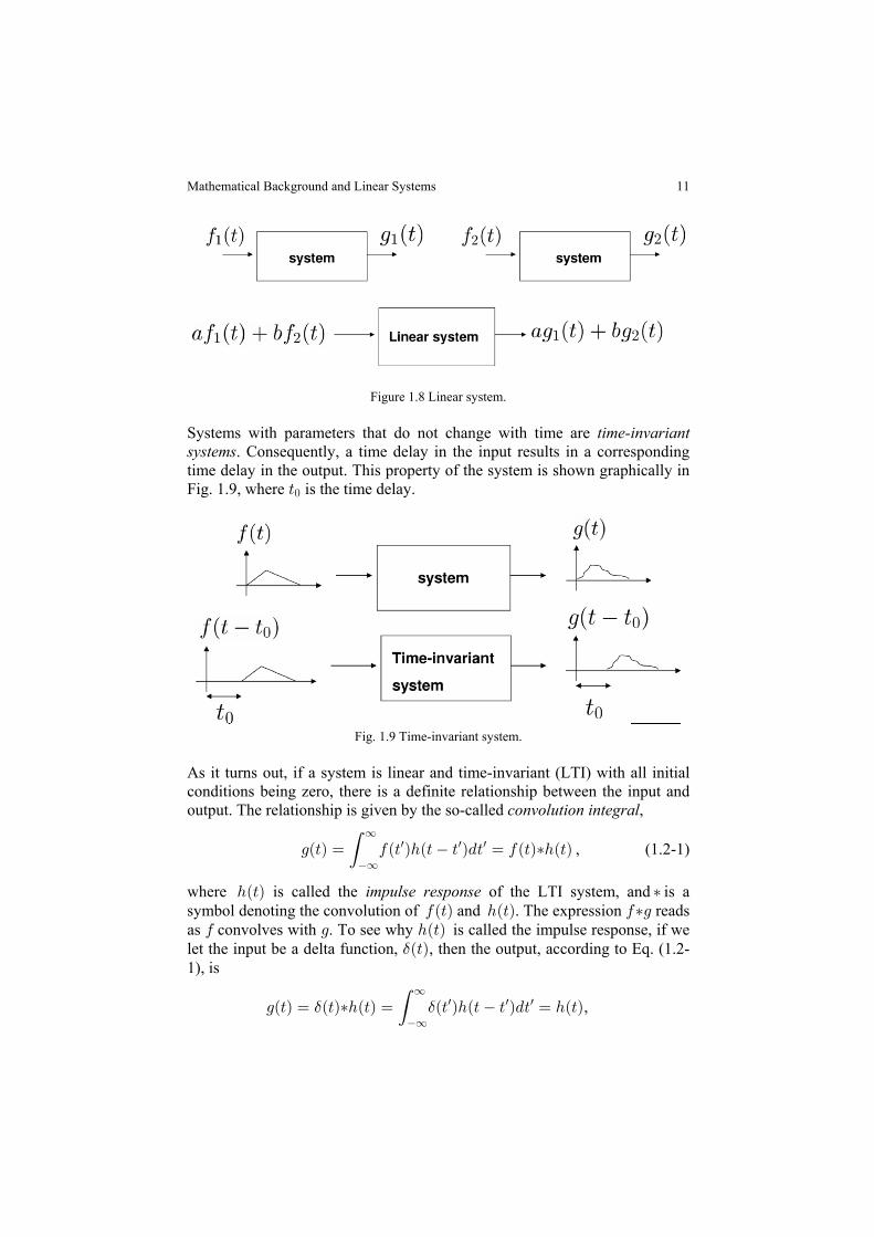
A system is defined as the mapping of an input or set of inputs into an outputor set of outputs. A system is linear if applies. For a single-superpositioninput single-output system, if an input gives an output of 0 Ð>Ñ" 1 Ð>Ñ" , and ifanother input , then superposition means if the0 Ð>Ñ# gives an output of 1 Ð>Ñ#

input is given by + +10 Ð>Ñ ,0 Ð>Ñ Ð>Ñ ,1 Ð>Ñß" # " #, the system s output is where and are some constants. The situation of a is further+ , linear systemillustrated in Fig. 1.8.

sents an idealized point source of light in optics. According to Eq. (1.1-2a),the 2-D Fourier transform of $ÐBß CÑ is given by

’


engineering, the 2-D version of a delta function, $ÐBß CÑ œ $ÐBÑ$ÐCÑ, repre-

11

Figure 1.8 Linear system.

Systems with parameters that do not change with time are time-invariantsystems. Consequently, a time delay in the input results in a correspondingtime delay in the output. This property of the system is shown graphically inFig. 1.9, where is the time delay.>!

Fig. 1.9 Time-invariant system.

As it turns out, if a system is linear and time-invariant (LTI) with all initialconditions being zero, there is a definite relationship between the input andoutput. The relationship is given by the so-called convolution integral,

1Ð>Ñ œ 0Ð> Ñ2Ð> > Ñ.> œ 0Ð>Ñ‡2Ð>Ñ(_

_w w w , (1.2-1)

where is called the of the LTI system, and is a2Ð>Ñ ‡impulse response symbol denoting the convolution of and . The expression reads0Ð>Ñ 2Ð>Ñ 0‡1as convolves with . To see why is called the impulse response, if we0 1 2Ð>Ñlet the input be a delta function, , then the output, according to Eq. (1.2-$Ð>Ñ1), is

1Ð>Ñ œ Ð>Ñ‡2Ð>Ñ œ Ð> Ñ2Ð> > Ñ.> œ 2Ð>Ñ$ $(_

_w w w ,


12

where we use the sampling property of the delta function to obtain the laststep of the result. Once we know of the LTI system, which can be2Ð>Ñdetermined experimentally by simply applying an impulse to the input of thesystem, we can find the response to any arbitrary input, say, to the0Ð>Ñßsystem through the calculation of Eq. (1.2-1).

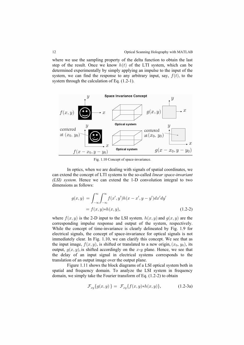
Fig. 1.10 Concept of space-invariance.

In optics, when we are dealing with signals of spatial coordinates, wecan extend the concept of LTI systems to the so-called linear space-invariant(LSI) system. Hence we can extend the 1-D convolution integral to twodimensions as follows:

1ÐBß CÑ œ 0ÐB ß C Ñ2ÐB B ß C C Ñ.B .C( (_ _

_ _w w w w w w

, (1.2-2)œ 0ÐBß CÑ‡2ÐBß CÑ

where is the 2-D input to the LSI system. and are the0ÐBß CÑ 2ÐBß CÑ 1ÐBß CÑcorresponding impulse response and output of the system, respectively.While the concept of time-invariance is clearly delineated by Fig. 1.9 forelectrical signals, the concept of space-invariance for optical signals is notimmediately clear. In Fig. 1.10, we can clarify this concept. We see that asthe input image, , is shifted or translated to a new origin, , , its0ÐBß CÑ ÐB C Ñ! !

output, , is shifted accordingly on the - plane. Hence, we see that1ÐBß CÑ B Cthe delay of an input signal in electrical systems corresponds to thetranslation of an output image over the output plane. Figure 1.11 shows the block diagrams of a LSI optical system both inspatial and frequency domain. To analyze the LSI system in frequencydomain, we simply take the Fourier transform of Eq. (1.2-2) to obtain

, (1.2-3a)Y YBC BCÖ Ö1ÐBß CÑ × œ 0ÐBß CÑ‡2ÐBß CÑ×


13

which is shown to be

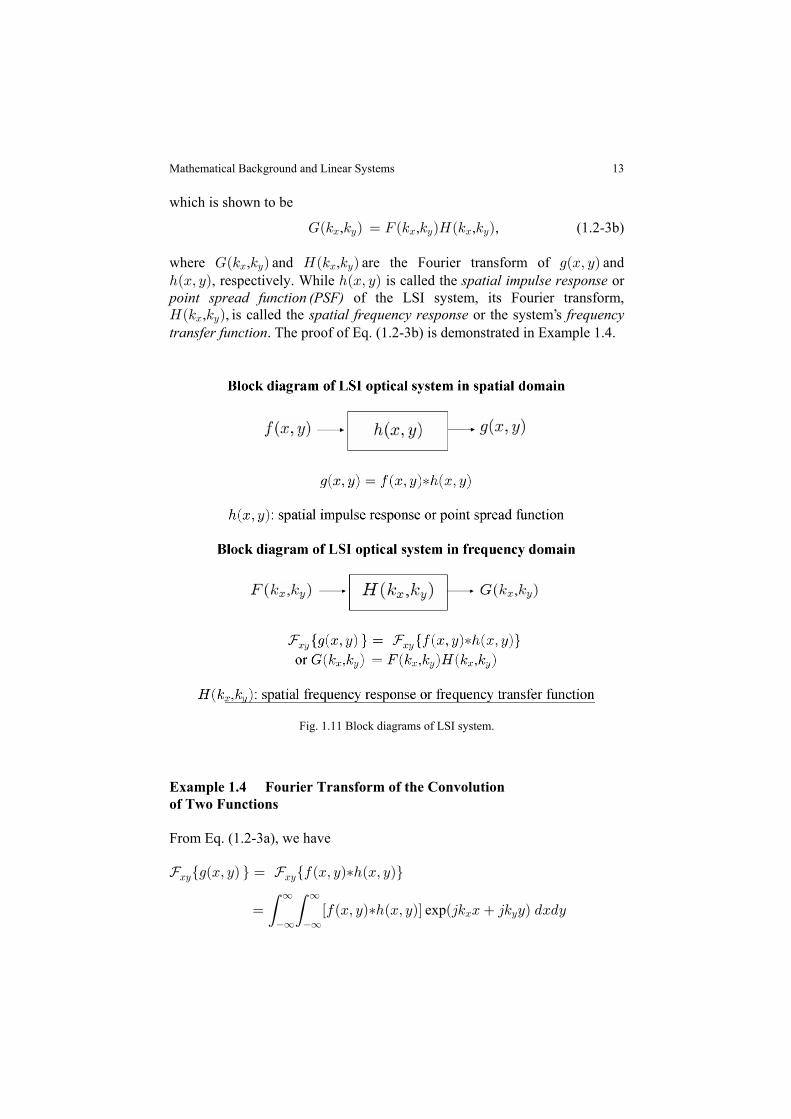
KÐ5 5 Ñ œ JÐ5 5 ÑLÐ5 5 ÑB C B C B C, , , , (1.2-3b)

where , and , are the Fourier transform of andKÐ5 5 Ñ LÐ5 5 Ñ 1ÐBß CÑB C B C

2ÐBß CÑ 2ÐBß CÑ, respectively. While is called the orspatial impulse responsepoint spread function (PSF) of the LSI system, its Fourier transform,LÐ5 5 ÑB C, , is called the or the system sspatial frequency response frequencytransfer function. The proof of Eq. (1.2-3b) is demonstrated in Example 1.4.

Fig. 1.11 Block diagrams of LSI system.

Example 1.4 Fourier Transform of the Convolutionof Two Functions

From Eq. (1.2-3a), we have

Y YBC BCÖ Ö1ÐBß CÑ × œ 0ÐBß CÑ‡2ÐBß CÑ×

œ Ò0ÐBß CÑ‡2ÐBß CÑÓ Ð45 B 45 CÑ .B.C( (_ _

_ _

B Cexp

’


14

œ 0ÐB ß C Ñ2ÐB B ß C C Ñ.B .C( ( ( (’ “_ _ _ _

_ _ _ _w w w w w w

exp ,‚ Ð45 B 45 CÑ .B.CB C

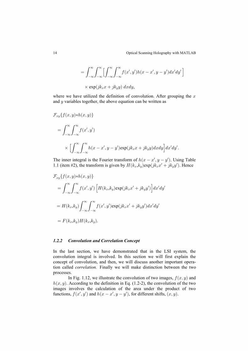
where we have utilized the definition of convolution. After grouping the Band variables together, the above equation can be written asC

YBCÖ ×0ÐBß CÑ‡2ÐBß CÑ

œ 0ÐB ß C Ñ( (_ _

_ _w w

‚ 2ÐB B ß C C Ñ Ð45 B 45 CÑ.B.C .B .C’ “( (_ _

_ _w w w w

B Cexp .

The inner integral is the Fourier transform of . Using Table2ÐB B ß C C Ñw w

1.1 (item #2), the transform is given by , exp . HenceLÐ5 5 Ñ Ð45 B 45 C ÑB C B Cw w

YBCÖ0ÐBß CÑ‡2ÐBß CÑ×

œ 0ÐB ß C Ñ LÐ5 5 Ñ Ð45 B 45 C Ñ .B .C( ( ’ “_ _

_ _w w w w w w

B C B C, exp

œ LÐ5 5 Ñ 0ÐB ß C Ñ Ð45 B 45 C Ñ.B .CB C B C_ _

_ _w w w w w w, exp( (

œ JÐ5 5 ÑLÐ5 5 ÑB C B C, , .

1.2.2 Convolution and Correlation Concept

In the last section, we have demonstrated that in the LSI system, theconvolution integral is involved. In this section we will first explain the

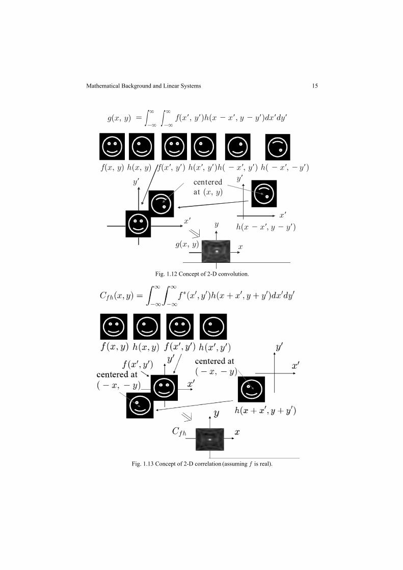
In Fig. 1.12, we illustrate the convolution of two images, and0ÐBß CÑ2ÐBß CÑ. According to the definition in Eq. (1.2-2), the convolution of the twoimages involves the calculation of the area under the product of twofunctions, and , for different shifts, .0ÐB ß C Ñ 2ÐB B ß C C Ñ ÐBß CÑw w w w

concept of convolution, and then, we will discuss another important opera-tion called correlation. Finally we will make distinction between the twoprocesses.


15

Fig. 1.12 Concept of 2-D convolution.

Fig. 1.13 Concept of 2-D correlation (assuming is real).0


g(x, y)

g(x, y)

f(x, y) h(x, y) f(x9, y9) h(x9, y9)h( 2 x9, y9) h( 2 x9, 2 y9)

f(x9, y9)h(x 2 x9, y 2 y9)dx9dy9

h(x 2 x9, y 2 y9)

= ∫ ∫`

2`

`

2`

x9x9

y9

y

x

y9 centeredat (x, y)

16

The first row of figures in Fig. 1.12 shows the construction of and0ÐB ß C Ñw w

2Ð B ß C Ñ 0ÐBß CÑ 2ÐBß CÑw w from the original images and . We thenconstruct as shown in Fig. 1.12 by translating2ÐB B ß C C Ñw w

2Ð B ß C Ñ ÐBß CÑ 2ÐB B ß C C Ñw w w w to a center at to form . Once we have0ÐB ß C Ñ 2ÐB B ß C C Ñ B Cw w w w w w and , we superimpose them on the - plane asillustrated in Fig. 1.12. Finally, we need to calculate the area of the productof and for different shifts to obtain a 2-D0ÐB ß C Ñ 2ÐB B ß C C Ñ ÐBß CÑw w w w

gray-scale plot of .1ÐBß CÑ Another important integral is called the . correlation integral Thecorrelation, , of two functions and , is defined asG ÐBß CÑ 0ÐBß CÑ 2ÐBß CÑ02

G ÐBß CÑ œ 0 ÐB ß C Ñ2ÐB B ß C C Ñ.B .C02_ _

_ _‡ w w w w w w( (

. (1.2-4)œ 0ÐBß CÑ Œ 2ÐBß CÑ

This integral is useful when comparing the similarity of two functions, and ithas been knowingly used for applications in pattern recognition. Forsimplicity, if we assume in Fig. 1.13 that is real,0ÐBß CÑ we can illustrate thecorrelation of the two images, and . Similar to the convolution0ÐBß CÑ 2ÐBß CÑof the two images, the correlation involves the calculation of the area underthe product of two functions, and , for different0ÐB ß C Ñ 2ÐB B ß C C Ñw w w w

shifts, . The first row of images in Fig. 1.13 shows the construction ofÐBß CÑ0ÐB ß C Ñ 2ÐB ß C Ñ 0ÐBß CÑ 2ÐBß CÑw w w w and from the original images, and . Unlikeconvolution, to calculate he area of the product of and0ÐB ß C Ñw w

2ÐB B ß C C Ñ ÐBß CÑw w for different shifts , , there is no need to flip the image,2ÐB ß C Ñ B Cw w w w, upon the - axis and the -axis to obtain the 2-D plot of .G ÐBß CÑ02

Example 1.5 Relationship between Convolution and Correlation

In this example, we will show that correlation can be expressed in terms ofconvolution through the following relationship:

0ÐBß CÑ Œ 2ÐBß CÑ œ 0 Ð Bß CÑ‡2ÐBß CÑ‡ . (1.2-5)

According to the definition of convolution [see Eq. (1.2-2)], we write

0 Ð Bß CÑ‡2ÐBß CÑ‡

œ 0 Ð B ß C Ñ2ÐB B ß C C Ñ.B .C( (_ _

_ _‡ w w w w w w


17

œ 0 ÐB Bß C CÑ2ÐB ß C ÑÐ .B ÑÐ .C Ñ( (_ _

_ _‡ ww ww ww ww ww ww ,

where we have made the substitutions and to obtainB B œ B C C œ Cw ww w ww

the last step of the equation. By re-arranging the last step and substituting theequivalents for and , we obtain B B œ B C C œ Cww wwμ μ

0 Ð Bß CÑ‡2ÐBß CÑ‡

œ 0 ÐBß CÑ2ÐB Bß C CÑ.B.C( (_ _

_ _‡ μ μ μ μ μ μ,

œ 0ÐBß CÑ Œ 2ÐBß CÑ

by the definition of correlation. Therefore, we have proven Eq. (1.2-5).

With reference to Eq. (1.2-4), when , the result is known as 0 Á 2 cross-correlation auto-correlation, When , the result is known as , G G02 00Þ 0 œ 2 ,of the function As it turns out, we can show that0Þ

l lG Ð!ß !Ñl G ÐBß CÑl00 00 , (1.2-6)

i.e., autocorrelation always has a central maximum. The use of this fact hasbeen employed by pattern recognition. Pioneering schemes of optical patternrecognition, implementing Eq. (1.2-5), are due to Vander Lugt [1964], andWeaver and Goodman [1966]. The book, ,Optical Pattern Recognitionprovides a comprehensive review of optical pattern recognition, coveringtheoretical aspects and details of some practical implementations [Yu andJutamulia (1998)]. For some of the most novel approaches to optical patternrecognition, the reader is encouraged to refer to the article by Poon and Qi[2003].

Example 1.6 MATLAB Example: Pattern Recognition

For pattern recognition applications, one implements correlation given by Eq.(1.2-4). In this example, we implement the equation in the frequency domain.To do this, we realize that

YBCÖ0ÐBß CÑ Œ 2ÐBß CÑ× œ J Ð5 5 ÑLÐ5 5 Ñ‡B C B C, , , (1.2-7)

which can be shown using the procedure similar to Example 1.4. For thegiven images and , we first find their corresponding 2-D Fourier0 2


18

transforms, and then the correlation is evident when we take the inversetransform of Eq. (1.2-7):

0ÐBß CÑ Œ 2ÐBß CÑ œ J Ð5 5 ÑLÐ5 5 Ñ×YBC"Ö ‡

B C B C, , . (1.2-8)

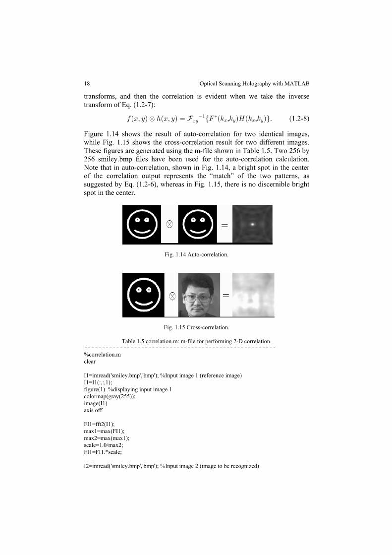
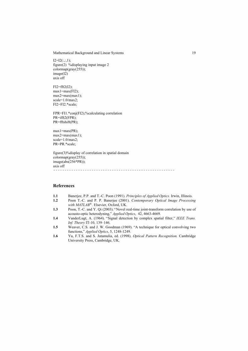
Figure 1.14 shows the result of auto-correlation for two identical images,while Fig. 1.15 shows the cross-correlation result for two different images.These figures are generated using the m-file shown in Table 1.5. Two 256 by256 smiley.bmp files have been used for the auto-correlation calculation.Note that in auto-correlation, shown in Fig. 1.14, a bright spot in the centerof the correlation output represents the match of the two patterns, assuggested by Eq. (1.2-6), whereas in Fig. 1.15, there is no discernible brightspot in the center.

Fig. 1.14 Auto-correlation.

Fig. 1.15 Cross-correlation.

Table 1.5 correlation.m: m-file for performing 2-D correlation.------------------------------------------------------%correlation.mclear

I1=imread('smiley.bmp','bmp'); %Input image 1 (reference image)I1=I1(:,:,1);figure(1) %displaying input image 1colormap(gray(255));image(I1)axis off

FI1=fft2(I1);max1=max(FI1);max2=max(max1);scale=1.0/max2;FI1=FI1.*scale;

I2=imread('smiley.bmp','bmp'); %Input image 2 (image to be recognized)

“ ”


19

I2=I2(:,:,1);figure(2) %displaying input image 2colormap(gray(255));image(I2)axis off

FI2=fft2(I2);max1=max(FI2);max2=max(max1);scale=1.0/max2;FI2=FI2.*scale;

FPR=FI1.*conj(FI2);%calculating correlationPR=ifft2(FPR);PR=fftshift(PR);

max1=max(PR);max2=max(max1);scale=1.0/max2;PR=PR.*scale;

figure(3)%display of correlation in spatial domain colormap(gray(255));image(abs(256*PR));axis off------------------------------------------------------

References

1.1 Banerjee, P.P. and T.-C. Poon (1991). Irwin, Illinois.Principles of Applied Optics.1.2 Poon T.-C. and P. P. Banerjee (2001). Contemporary Optical Image Processing

with MATLAB . ® Elsevier, Oxford, UK.1.3 Poon, T.-C. and Y. Qi (2003). Novel real-time joint-transform correlation by use of

acousto-optic heterodyning, , 42, 4663-4669.Applied Optics1.4 VanderLugt, A. (1964). Signal detection by complex spatial filter, IEEE Trans.

Inf. Theory IT-10, 139–146.1.5 Weaver, C.S. and J. W. Goodman (1969). A technique for optical convolving two

functions, , 5, 1248-1249.Applied Optics1.6 Yu, F.T.S. and S. Jutamulia, ed. (1998). CambridgeOptical Pattern Recognition.

University Press, Cambridge, UK.

“”

“ ”

“”


Chapter 2

Wave Optics and Holography

In Chapter 1, we presented some mathematical background of Fourier opticsas well as some important systems properties including linearity and spaceinvariance. In this chapter, we present some fundamentals of wave optics bystarting from Maxwell s equations and deriving the vector wave equation. We

response in Fourier optics. In the context of diffraction, we will also developwavefront transformation by using a lens, show the Fourier transformingproperties of the lens, and discuss how spatial filtering is obtained by using astandard two-lens system, leading to the distinction between coherent andincoherent image processing. In the last section of this chapter, we willdiscuss the basics of holography and show that a Fresnel zone plate is thehologram of a point source object, leading to the concept that the hologramof an arbitrary 3-D object can be considered as a collection of Fresnel zoneplates. Finally, we will discuss electronic holography (often called digitalholography in literature). This will culminate with the next chapter, which wewill discuss a unique holographic recording technique called optical scanningholography.

2.1 Maxwell s Equations and Homogenous Vector Wave Equation

Generally, in the study of optics, we are concerned with four vectorquantities called electromagnetic (EM) fields: the electric field strength X(V/m), the electric flux density (C/m ), the magnetic field strength W # [(A/m), and the magnetic flux density (Wb/m ). The fundamental theory ofU #

electromagnetic fields is based on Maxwell s Equations. In differential form,these equations are expressed as

f † œW 3@ , (2.1-1)

f † œ !U , (2.1-2)

we will develop diffraction theory by using the Fresnel diffraction for-will then discuss some simple solutions of the scalar wave equation. Next,

mula, which is uniquely derived by using Fourier transforms. In the process, we will define the spatial frequency transfer function and the spatial impulse

’

’

’

f‚ X œ

U

t , (2.1-3)

, (2.1-4)f‚[ œ œ ] ]W

-

t

where is the current density [A/m ] and denotes the electric charge] 3-#

@ density [C/m ]. and are the sources generating the electromagnetic3 ] 3- @

fields. Maxwell s equations express the physical laws governing the electricfields magnetic fields sources , and the and . FromX [ U and and , W ] 3 - @

Eqs. (2.1-3) and (2.1-4), we see that a time-varying magnetic field produces atime-varying electric field. Conversely, a time-varying electric field producesa time-varying magnetic field. It is precisely this coupling between theelectric and magnetic fields that generate electromagnetic waves capable ofpropagating through a medium or even in free space.

For any given current and charge density distribution, we can solveMaxwell s equations. However, we need to note that Eq. (2.1-1) is notindependent of Eq. (2.1-4). Similarly, Eq. (2.1-2) is a consequence of Eq.(2.1-3). By taking the divergence on both sides of Eqs. (2.1-3) and (2.1-4)and using the continuity equation:

f † œ]3

- +

@

t0, (2.1-5)

which is the we can show thatprinciple of conservation of charge,f †W œ 3

@ . Similarly, Eq. (2.1-2) is a consequence of Eq. (2.1-3). Hence, from Eqs. (2.1-1) to (2.1-4), we really have six independent scalar equations(three scalar equations for each curl equation) and twelve unknowns. Theunknowns are the and components of , , , and . The six moreBß Cß D X [ UWscalar equations required are provided by the :constitutive relations

, (2.1-6a)W Xœ %and U [œ . , (2.1-6b)

where denotes the permittivity [F/m] and denotes the permeability [H/m]% . of the medium. In this book, we take and to be scalar constants. Indeed,% .this is true for a , , and medium. A medium islinear homogeneous isotropiclinear if its properties do not depend on the amplitude of the fields in themedium. It is if its properties are not functions of space. Andhomogeneousthe medium is if its properties are the same in all direction from anyisotropicgiven point. Returning our focus to linear, homogeneous, and isotropic media,constants worth remembering are the values of and for free space (or% .vacuum): (1/36 ) 10 F/m and 4 10 H/m.% 1 . 1! !

* œ ‚ œ ‚ 7

22

’

’


23

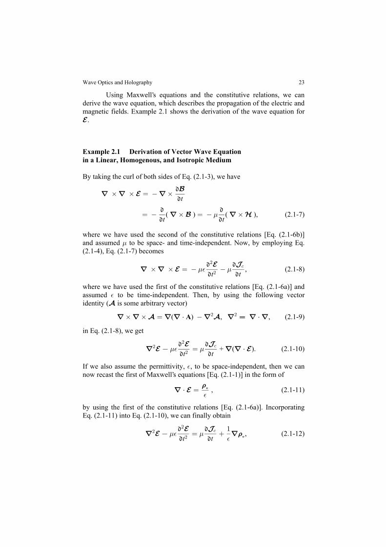
Using Maxwell s equations and the constitutive relations, we canderive the wave equation, which describes the propagation of the electric andmagnetic fields. Example 2.1 shows the derivation of the wave equation forX .

Example 2.1 Derivation of Vector Wave Equationin a Linear, Homogenous, and Isotropic Medium

By taking the curl of both sides of Eq. (2.1-3), we have

f f f‚ ‚ œ ‚X

U

t

( ) ( ), (2.1-7)œ œ

.

t tf f‚ ‚U [

where we have used the second of the constitutive relations [Eq. (2.1-6b)]and assumed to be space- and time-independent. Now, by employing Eq..(2.1-4), Eq. (2.1-7) becomes

f f ‚ ‚ œ X .% .

#-X ]

t t#, (2.1-8)

where we have used the first of the constitutive relations [Eq. (2.1-6a)] andassumed to be time-independent. Then, by using the following vector%identity ( is some arbitrary vector)T

f f f f † f f œ f †f‚ ‚ œ T T( ) , , (2.1-9)A # #

in Eq. (2.1-8), we get

f f f †#X X.%

.

#-X ]

t t#œ + ( ). (2.1-10)

If we also assume the permittivity, , to be space-independent, then we can%now recast the first of Maxwell s equations [Eq. (2.1-1)] in the form of

f † X œ3

@

%, (2.1-11)

by using the first of the constitutive relations [Eq. (2.1-6a)]. IncorporatingEq. (2.1-11) into Eq. (2.1-10), we can finally obtain

f f#X .%

%.

#-X ]

3t t#

œ "

@, (2.1-12)

’

’


24

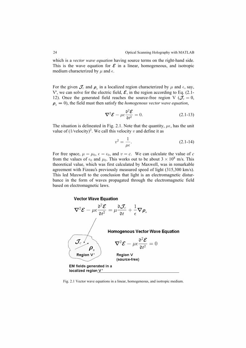
which is a having source terms on the right-hand side.vector wave equationThis is the wave equation for in X a linear, homogeneous, and isotropicmedium characterized by . % and .

For the given and in a localized region and , say,] 3- @ characterized by . %

we can solve for the electric field, , in the region according to Eq. (2.1-X 12). Once the generated field reaches the source-free region V 0,(]- œ3

@œ 0), the field must then satisfy the homogenous vector wave equation,

f #X .%

#X

t#œ !. (2.1-13)

The situation is delineated in Fig. 2.1. Note that the quantity, , has the unit.%value of (1/velocity) . We call this velocity # @ and define it as

@# œ"

.%. (2.1-14)

For free space, , , and . We can calculate the value of . . % %œ œ! ! @ œ c cfrom the values of and . This works out to be about 3 10 m/s. This% .! ! ‚ 8

theoretical value, which was first calculated by Maxwell, was in remarkableagreement with Fizeau s previously measured speed of light (315,300 km/s).

Fig. 2.1 Vector wave equations in a linear, homogeneous, and isotropic medium.

’This led Maxwell to the conclusion that light is an electromagnetic distur-bance in the form of waves propagated through the electromagnetic fieldbased on electromagnetic laws.

V',


25

2.2 Three-Dimensional Scalar Wave Equation

Equation (2.1-13) is equivalent to three scalar equations - one for everycomponent of . to be of the formX XWe shall let the field

X œ X X XB B C C D Da a a + , (2.2-1)

where a a aB C D, , and denote the unit vectors in the , , and directions,B C Drespectively. Now, the expression for the Laplacian ( ) operator inf#

Cartesian ( ) coordinates is given byBß Cß D

f# œ

# # #

B C# # # + + .

D(2.2-2)

Using the above equation, Equation (2.1-13) becomes

Ð Ð Ñ

# # #

B C D# # # + + Ñ X X XB B C C D Da a a +

œ Ð Ñ.% X X X

#

t# B B C C D Da a a + . (2.2-3)

Comparing the -component on both sides of the equation, we haveaB

# # # #X X X X.%

B B B B

B C D# # # # + + œ

t.

Similarly, we end up with the same type of equation shown above for the XCand component by comparing the other components in Eq. (2.2-3).XDTherefore, we can write

f#< œ"

@#

#

<

t# (2.2-4),

where may represent a component, , or , of the electric field , and< X X XB C D X

Equation (2.2-4) is called the We shall look at3-D scalar wave equation.some of its simplest solutions in the next section.

2.2.1 Plane Wave Solution

For waves oscillating at the , (rad/s), one of theangular frequency =!

simplest solutions to Eq. (2.2-4) is

, , , exp< =Ð Ò4Ð B C D Ñt tœ 5! ! † VÑÓ


where @ is the velocity of the wave in the medium by using Eq. (2.1-14).

26

exp , (2.2-5)œ Ò4Ð =! !B !C !Dt k k kB C DÑÓ

where + + is the position vector, V œ B C Da a a a aB C D B C5! !B !Cœ k k + +k propagation vector k propagation!D ! !aD is the , and | | is called the 5 œconstant [rad/m]. With the condition that

= =2 2

2 2 2 2! !

!B !C !D !

#

k k k k+ + , (2.2-6)œ œ @

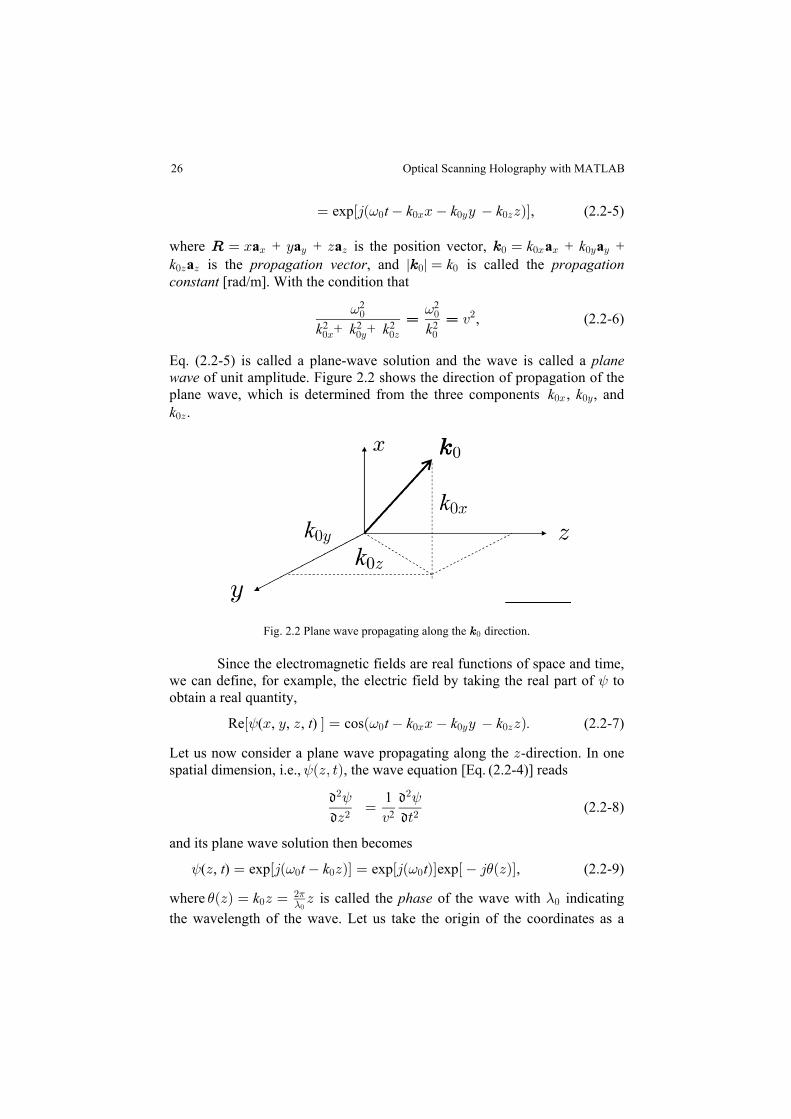
Eq. (2.2-5) is called a plane-wave solution and the wave is called a planewave of unit amplitude. Figure 2.2 shows the direction of propagation of theplane wave, which is determined from the three components , , andk k!B !C

k!D .

Fig. 2.2 Plane wave propagating along the 5! direction.

Since the electromagnetic fields are real functions of space and time,we can define, for example, the electric field by taking the real part of to<obtain a real quantity,

Re ( , , , ) cos (2.2-7)Ò Ó œ Ð < =B C D B C DÑt t k k k .! !B !C !D

Let us now consider a plane wave propagating along the -direction. In oneDspatial dimension, i.e.,<ÐDß >Ñ, the wave equation [Eq. (2.2-4)] reads

(2.2-8)1 < <

# #

D @ ># #œ 2

and its plane wave solution then becomes

, (2.2-9)< = = )( , ) exp exp expD DÑÓ œ ÑÓt t k tœ Ò4Ð Ò4Ð Ò 4 ÐDÑÓ! ! !

where is called the of the wave with indicating)ÐDÑ œ k phase !D œ D#!

1-!

-

the wavelength of the wave. Let us take the origin of the coordinates as a


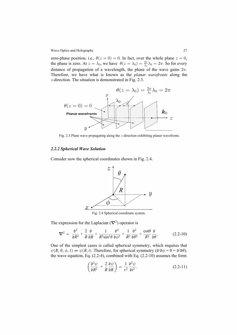
27

zero-phase position, i.e., In fact, over the whole plane ,)Ð D œ !D œ !Ñ œ !. the phase is zero. At , we have So for everyD œ D œ Ñ œ œ #- - - 1! ! !

# . )Ð 1-!

distance of propagation of a wavelength, the phase of the wave gains #1.

D

Fig. 2.3 Plane wave propagating along the -direction exhibiting planar wavefronts.D

2.2.2 Spherical Wave Solution

Consider now the spherical coordinates shown in Fig. 2.4.

Fig. 2.4 Spherical coordinate system.

The expression for the Laplacian ( ) operator isf#

(2.2-10)f# œ )

)

# # #

# #R R R R R R# # # # # + + + + .

2 cotsin" "

9 ) )

One of the spherical symmetrysimplest cases is called , which requires that< ) 9 < 9 )Ð >Ñ ÐR R t, , , , . Therefore, for spherical symmetry ( / = 0 = / ),œ Ñthe wave equation, Eq. (2.2-4), combined with Eq. (2.2-10) assumes the form

+ . (2.2-11)2 1Œ < < <

2 2

2 2 2R R R tœ

@

-direction. The situation is demonstrated in Fig. 2.3.Therefore, we have what is known as the planar wavefronts along the


28

Since

RR R R R

RŒ < < <

2 2

2 2 + ,2

œÐ Ñ

we can re-write Eq. (2.2-11) to become

< <

2 2

2 2 2Ð Ñ Ð Ñ

œR RR t

1. (2.2-12)

@

Now, the above equation is of the same form as that of Eq. (2.2-8). Since Eq.(2.2-9) is the solution to Eq. (2.2-8), we can therefore construct a simplesolution to Eq. (2.2-12) as

< =Ð œ Ò4Ð R t t k R, exp , (2.2-13)Ñ ÑÓ"

V! !

which is called a Again, we can writespherical wave.

< = = )( , ) exp exp exp ,R t t k R t Rœ Ò4Ð œ Ð4 Ò 4 Ð ÑÓ" "

V VÑÓ Ñ! ! !

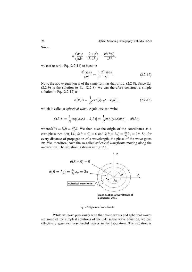
where We then take the origin of the coordinates as a)Ð Ñ œR k R R.! œ #1-!

zero-phase position, i.e., and So, for) )Ð ÐR R . œ !Ñ œ ! œ Ñ œ œ #- - 1! !#1-!

every distance of propagation of a wavelength, the phase of the wave gains#1. spherical wavefrontsWe, therefore, have the so-called moving along theR-direction. The situation is shown in Fig. 2.5.

Fig. 2.5 Spherical wavefronts.

While we have previously seen that plane waves and spherical wavesare some of the simplest solutions of the 3-D scalar wave equation, we caneffectively generate these useful waves in the laboratory. The situation is


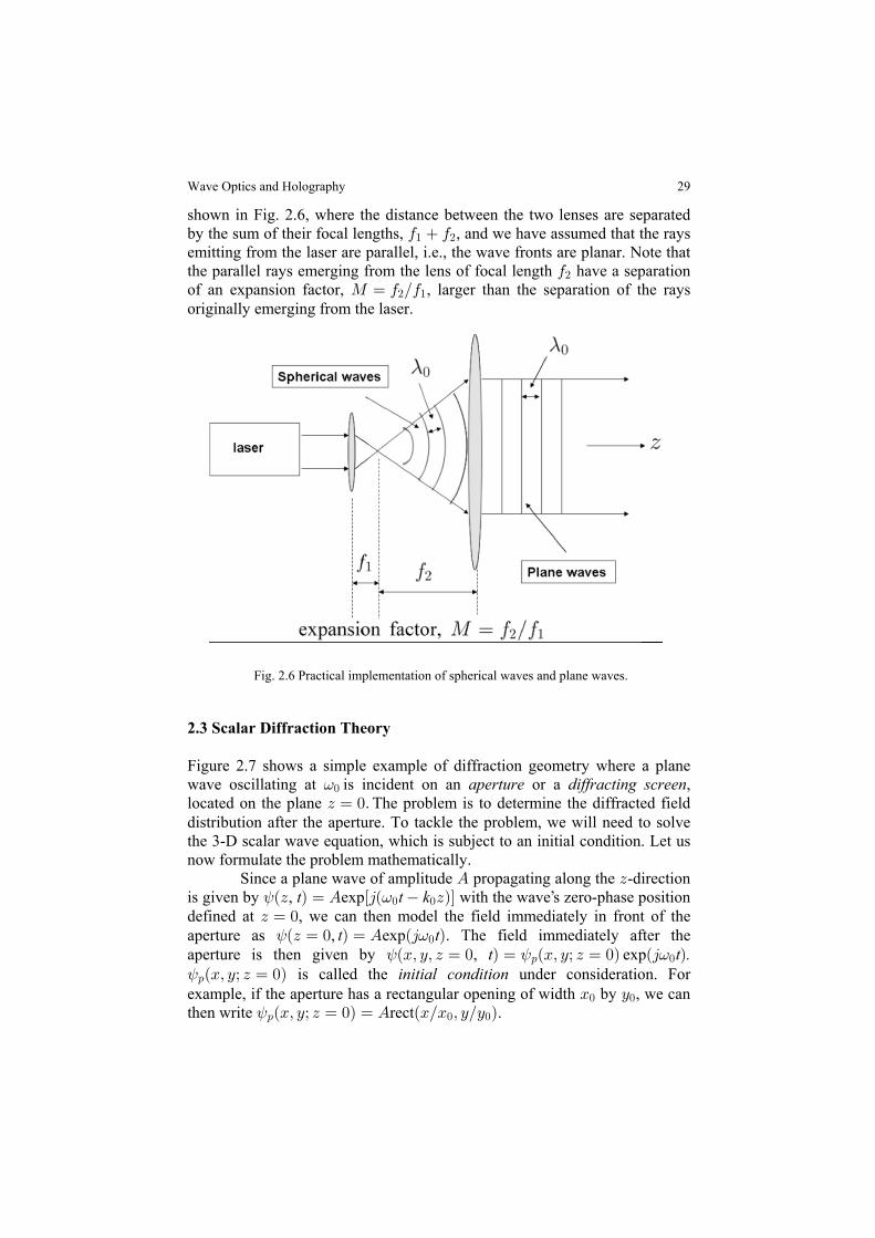
29

shown in Fig. 2.6, where the distance between the two lenses are separatedby the sum of their focal lengths, , and we have assumed that the rays0 0" #

emitting from the laser are parallel, i.e., the wave fronts are planar. Note thatthe parallel rays emerging from the lens of focal length have a separation0#of an expansion factor, , larger than the separation of the raysQ œ 0 Î0# "

originally emerging from the laser.

Fig. 2.6 Practical implementation of spherical waves and plane waves.

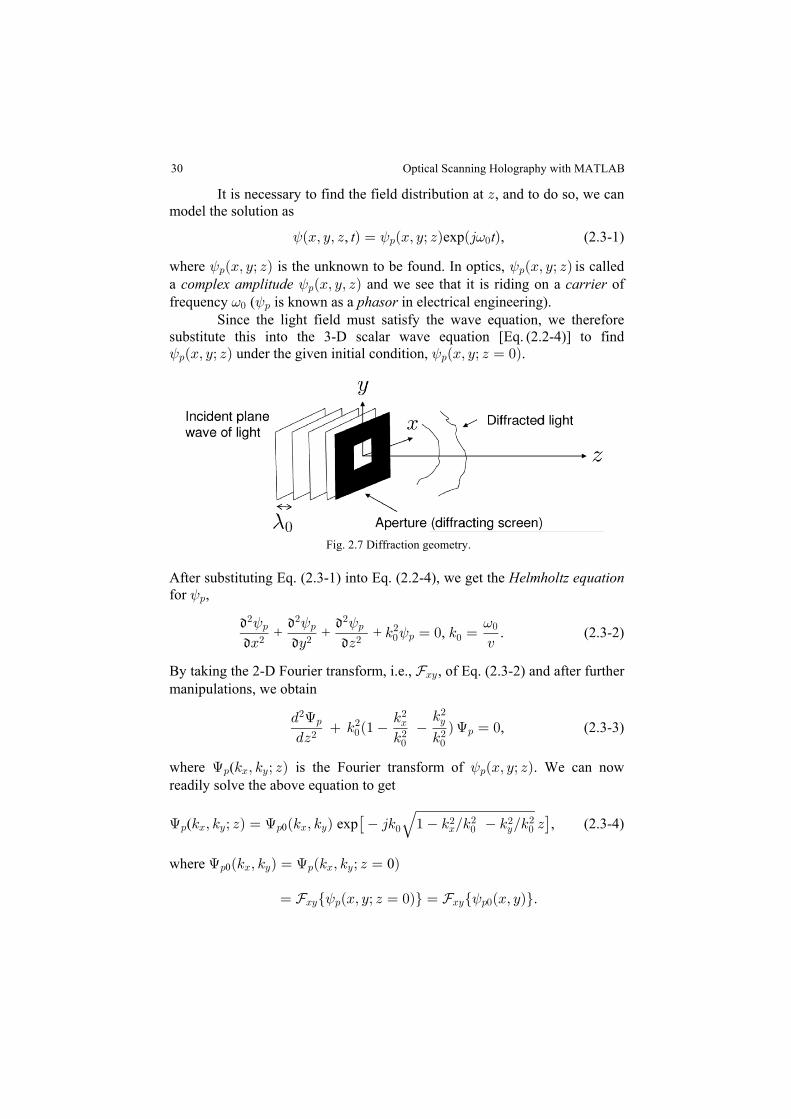
2.3 Scalar Diffraction Theory

Figure 2.7 shows a simple example of diffraction geometry where a planewave oscillating at is incident on an or a ,=! aperture diffracting screenlocated on the plane The problem is to determine the diffracted fieldD œ !Þdistribution after the aperture. To tackle the problem, we will need to solvethe 3-D scalar wave equation, which is subject to an initial condition. Let usnow formulate the problem mathematically. Since a plane wave of amplitude propagating along the -directionE Dis given by < =Ð œ E Ò4Ð D Ñ DÑÓ, exp with the wave s zero-phase positiont t k ! !

defined at , we can then model the field immediately in front of theD œ !aperture as , exp . The field immediately after the< =Ð œ E Ð4D œ ! Ñ Ñt t!aperture is then given by , exp< < =ÐBß Cß œ ÐBß Cà Ð4D œ ! Ñ D œ !Ñ Ñt t .: !

<:ÐBß Cà D œ !Ñ is called the under consideration. Forinitial conditionexample, if the aperture has a rectangular opening of width by , we canB C! !

then write rect .<: ! !ÐBß Cà œ E ÐBÎB ß CÎC ÑD œ !Ñ

’


30

It is necessary to find the field distribution at , and to do so, we canDmodel the solution as

< < =ÐBß Cß œ ÐBß Cà Ð4D Ñ DÑ Ñ, exp , (2.3-1)t t: !

where is the unknown to be found. In optics, is called< <: :ÐBß Cà ÐBß CàDÑ DÑ a and we see that it is riding on a ofcomplex amplitude carrier <:ÐBß Cß DÑfrequency ( is known as a in electrical engineering).= <! : phasor Since the light field must satisfy the wave equation, we thereforesubstitute this into the 3-D scalar wave equation [Eq. (2.2-4)] to find< <: :ÐBß Cà ÐBß CàDÑ D œ !Ñ under the given initial condition, .

Fig. 2.7 Diffraction geometry.

After substituting Eq. (2.3-1) into Eq. (2.2-4), we get the Helmholtz equationfor <:,

,

# # ##! !

< < < =<

: : : !:

B C D @5 5 œ

# # # + + + . (2.3-2)œ !

By taking the 2-D Fourier transform, i.e., , of Eq. (2.3-2) and after furtherYBC

manipulations, we obtain

. 5

.D 5 Ð" Ñ

5 5

5# ##!

B# #! !

#CGG

::#

(2.3-3)œ !,

where ( is the Fourier transform of . We can nowG <: B C :5 ß 5 à DÑ ÐBß Cà DÑreadily solve the above equation to get

G G: B C : B C( exp5 ß 5 à DÑ œ Ð5 ß 5 Ñ 40 5 " 5 Î5 5 Î5 D!# #B C

# #! !É ‘, (2.3-4)

where 0G G: B C : B C0Ð5 ß 5 Ñ œ Ð5 ß 5 à D œ Ñ

.œ ÐBß Cà D œ !Ñ× œ ÐBß CÑ×Y YBC BCÖ Ö< <: :!


31

We can interpret Eq. (2.3-4) by considering a linear system with (G: B C0 5 ß 5 Ñas its input spectrum (i.e., at ) and where the output spectrum isD œ !G: B CÐ5 ß 5 à DÑ. Conclusively, the spatial frequency response of the system is

G

G[

: B C

: B CB C

Ð5 ß 5 à DÑ

Ð5 ß 5 Ñœ Ð5 ß 5 à DÑ

0

exp œ 4 5 " 5 Î5 5 Î5 D!# #B C

# #! !É ‘ . (2.3-5)

We call the [ Ð5 ß 5 à DÑB C spatial frequency transfer function of propagationof light through a distance in the medium. Figure 2.8 shows theDrelationship between the input spectrum and the output spectrum.

Fig. 2.8 Spatial frequency transfer function of propagationrelating input spectrum to output spectrum.

Example 2.2 Derivation of the Helmholtz Equation

When we substitute into the 3-D scalar< < =ÐBß Cß œ ÐBß Cà Ð4D Ñ DÑ Ñ, expt t: !

wave equation given by Eq. (2.2-4), we have

Ò Ó œÐ4

@

=

= < =

# # # #

! : !!

#

< < <: : :

B C DÐ4 ÐBß Cà Ð4

Ñ# # #

+ + exp exp t tÑ DÑ Ñ

or

Ò Ó œ œ

@

=

< <

# # # #!

# : :#!

< < <: : :

B C DÐBß Cà 5

# # # + + DÑ

which is the Helmholtz equation [Eq. (2.3-2)], where we have incorporatedthe fact that . Note that the Helmholtz equation contains no time5 œ @! =!/variable.

Example 2.3 Derivation of Eq. (2.3-3) and its Solution

By taking the 2-D Fourier transform, i.e., , of Eq. (2.3-2) and by usingYBC

item #5 of Table 1.1, we can obtain


given by

32

Y

BC

# # ##!Ö 5

B C D

< < <<

: : ::# # #

+ + +

× œ !

or

Ð5 5 Ñ Ð5 ß 5 à DÑ Ð5 ß 5 à DÑ œ !Ð5 ß 5 à DÑ# #

B C : B C : B C: B C

G GG.

.D 5

##!

,

#

which can then be re-arranged to become

. 5

.D 5 Ð" Ñ

5 5

5# ##!

B# #! !

#CGG

::#

œ !. (2.3-6)

This equation is of the form

.

.D C

##C

œ !#

! ,

which has the solution exp where is givenCÐDÑ œ C Ð 4 DÑ C œ CÐD œ !Ñ! !!as the initial condition. Using this result, the solution to Eq. (2.3-6) becomes

G G: B C B CÐ5 ß 5 à DÑ œ Ð5 ß 5 à D œ !Ñ 4exp 5 " 5 Î5 5 Î5 D!# #B C

# #! !É ‘

expœ Ð5 ß 5 Ñ 4G: B C0 5 " 5 Î5 5 Î5 D!# #B C

# #! !É ‘, (2.3-7)

which is Eq. (2.3-4).

To find the field distribution at in the spatial domain, we take the inverseDFourier transform of Eq. (2.3-7):

< G: : B CÐBß Cà DÑ œ Ð5 ß 5 à DÑY"BC š ›

œ 5 " 5 Î5 5 Î5 DÓ"

%Ð5 ß 5 Ñ 4

1G

# : B C( ( 0 exp ! B C# ## #

! !É exp . (2.3-8)‚ Ð 45 B 45 CÑ .5 .5B C B C

Now, by substituting we canG <: B C :!0( = into Eq. (2.3-8), 5 ß 5 Ñ ÐBß CÑYBCš ›


33

express as<:ÐBß Cà DÑ

< <: :!w w w w w wÐBß Cà DÑ œ ÐB ß C ÑKÐB B ß C C à DÑ .B .C ( (

, (2.3-9)œ ÐBß CÑ ‡KÐBß Cà DÑ<:!

where

KÐBß Cà DÑ œ 4"

%1#( ( exp 5 " 5 Î5 5 Î5 D! B C# ## #

! !É ‘

‚ Ð 45 B 45 CÑ .5 .5exp .B C B C

The result of Eq. (2.3-9) indicates that can be considered as theKÐBß Cà DÑspatial impulse response of propagation of light, which can be evaluated tobecome [Poon and Banerjee (2001)]

KÐBß Cà DÑ œ45 Ð 4 Ñ!exp

25 B C D

B C D!

# # #

# # #

ÈÈ1‚

B C D B C D

D "Ð" Ñ

45È È# # # # # #!

. (2.3-10)

2.3.1 Fresnel Diffraction

Equation (2.3-10) is complicated to use as is, and we shall need to make thefollowing approximations to obtain the well-known Fresnel diffractionformula commonly used in Fourier optics:

(1) For i.e., we observe the field distribution manyD ¦ œ # Î5 ß- 1! !

wavelengths away from the diffracting aperture, and we have

Ð" Ñ ¸"

45!ÈB C D# # # 1 .

(2) Using the binomial expansion, the factor

ÈB C D ¸ D B C

#D# # #

# #

,

provided that << . This condition is called the B C D# # # paraxialapproximation. If this approximation is used in the more sensitive phase termand only used the first expansion term in the less sensitive denominators of


34

the first and second terms of becomes the so-Eq. (2.3-10), then KÐBß Cà DÑcalled spatial impulse response in Fourier optics, [Poon and2ÐBß Cà DÑBanerjee (2001), Goodman (2005)]:

2ÐBß Cà DÑ œ Ð 45 DÑ45

# Dexp exp . (2.3-11)!

!

1’ 45 ÐB C Ñ

#D!

# # “If Eq. (2.3-11) is now used in Eq. (2.3-9), we obtain

< <: :!ÐBß Cà DÑ œ ÐBß CÑ ‡ 2ÐBß Cà DÑ

œ Ð 45 DÑ ÐB ß C Ñ45

# Dexp ! :!

! w w

1<( (

‚ Ö B B Ñ C C Ñ .B .Cexp . (2.3-12) 45

#DÒÐ Ð Ó×! # #w w w w+

Equation (2.3-12) is called the and describes theFresnel diffraction formula Fresnel diffraction of a beam during propagation and having an arbitraryinitial complex profile, <:!ÐBß CÑ. To obtain the output field distribution<:ÐBß Cà DÑ D at a distance away from the input (the location of the diffractingscreen), we would simply convolve the input field distribution, ,<:!ÐBß CÑ

with the spatial impulse response, .2ÐBß Cà DÑ By taking the 2-D , we obtain Fourier transform of 2ÐBß Cà DÑ

LÐ5 ß 5 à DÑ œ 2ÐBß Cà DÑB C YBCš ›œ Ð 45 DÑexp exp (2.3-13)! ’4 Ð5 5 ÑD

#5Þ

B C# #

!

“LÐ5 ß 5 à DÑB C is known as the spatial frequency transfer function in Fourieroptics. Indeed, we can derive Eq. (2.3-13) directly if we assume that5 5 ¥ 5 B CB C# # #

! , meaning that the and components of the propagationvector of a wave are relatively small, from Eq. (2.3-5), we have

G

G[

: B C

: B CB C

((5 ß 5 à DÑ

5 ß 5 Ñœ Ð5 ß 5 à DÑ

0

œ 4exp 5 " Ð5 5 ÑÎ5 D!# #B C

#!É ‘

¶4 Ð5 5 ÑD

#5 exp expÐ 45 DÑ! ’ B C

# #

!

“œ LÐ5 ß 5 à DÑB C


35

or

G G: B C : B C B C( ( . (2.3-14)5 ß 5 à DÑ œ 5 ß 5 ÑLÐ5 ß 5 à DÑ0

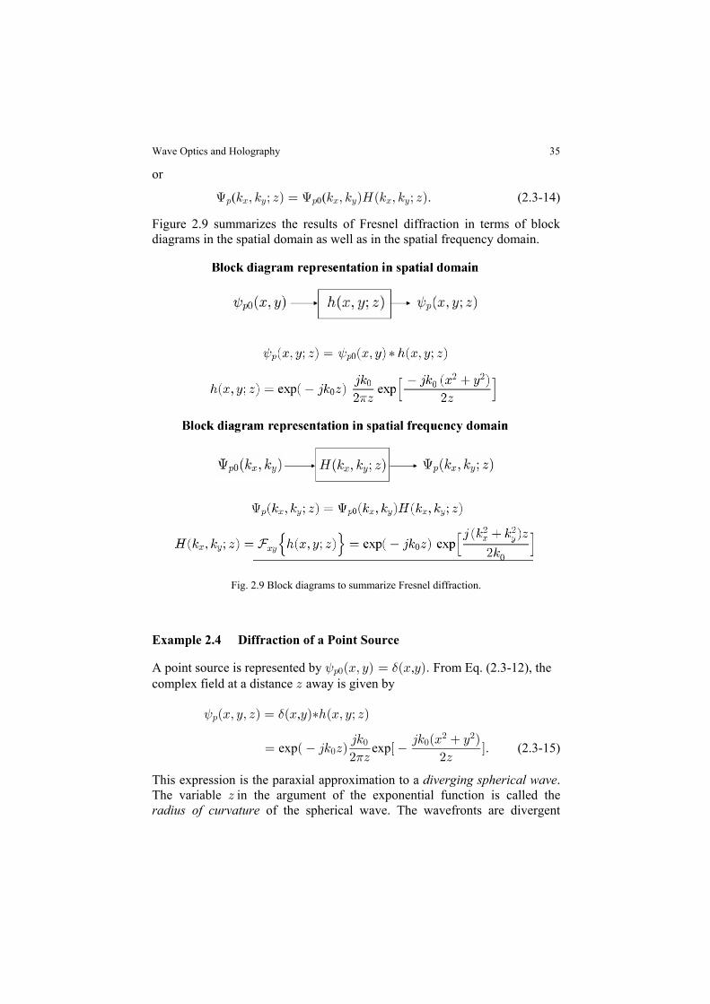
Figure 2.9 summarizes the results of Fresnel diffraction in terms of blockdiagrams in the spatial domain as well as in the spatial frequency domain.

Fig. 2.9 Block diagrams to summarize Fresnel diffraction.

Example 2.4 Diffraction of a Point Source

A point source is represented by , From Eq. (2.3-12), the< $:!ÐBß CÑ œ ÐB CÑÞcomplex field at a distance away is given byD

,< $:ÐBß Cß DÑ œ ÐB CÑ‡2ÐBß Cà DÑ

œ Ð 45 DÑ Ò Ó45 45 ÐB C Ñ

# D #Dexp exp . (2.3-15)!

! !# #

1

This expression is the paraxial approximation to a .diverging spherical waveThe variable in the argument of the exponential function is called theDradius of curvature of the spherical wave. The wavefronts are divergent


36

when and convergent when We can re-write Eq. (2.3-15) asD ! D !Þ

<1

: !!

# #

ÐBß Cß DÑ œ Ò 45 ÐD ÑÓ45 B C

# D #Dexp .

Now, by considering the argument of the exponential function, we see thatby using the binomial expansion , ÈB C D ¸ D # # # B C

#D we can write# #

<1

: !! # # #ÐBß Cß DÑ ¶ 45 B C D

45

# Dexp[ ( ) ]

"#

¶ Ð 45 VÑ45

# V!

!1

exp , (2.3-16)

where we have used in the less sensitive D ¶ V denominator. Eq. (2.3-16)corresponds to Eq. (2.2-13) for a cal wave.diverging spheri

Example 2.5 Diffraction of a Plane Wave

For a plane wave, we can write Then<p!ÐBß CÑ œ "ÞG 1 $ $:! B C B C

#Ð5 ß 5 Ñ œ % Ð5 Ñ Ð5 Ñ. Using Eq. (2.3-14), we have

exp exp G 1 $ $: B C B C !# B C

# #

!Ð5 ß 5 à DÑ œ % Ð5 Ñ Ð5 Ñ Ð 45 DÑ Ò Ó

4Ð5 5 ÑD

#5

exp .œ % Ð5 Ñ Ð5 Ñ Ð 45 DÑ1 $ $#B C !

Its inverse transform gives the expression of a plane wave [see Eq. (2.2-9)],

exp .<: !ÐBß Cß DÑ œ Ð 45 DÑ

As the plane wave travels, it only acquires phase shift and, as expected, isundiffracted.

2.3.2 Diffraction of a Square Aperture

In general, when a light field illuminates a transparency of transmissionfunction given by , and if the complex amplitude of the light just in>ÐBß CÑfront of the transparency is , then the complex field immediately<3ß:ÐBß CÑafter the transparency is given by . In writing this product<3ß:ÐBß CÑ>ÐBß CÑresult, we assume that the transparency is infinitely thin.


37

Now, let us consider a simple situation where a plane wave of unitamplitude is incident normally on the transparency , and the field>ÐBß CÑemerging from the transparency is then as in the" ‚ >ÐBß CÑ ÐBß CÑ œ "<3ß:

present case. We want to find the field distribution, which is a distance Daway from the transparency. This corresponds to the Fresnel diffraction of anarbitrary beam profile as the transparency modifies the incident plane wave.The situation is demonstrated in Fig. 2.10.

Fig. 2.10 Fresnel diffraction of an arbitrary beam profile .>ÐBß CÑ

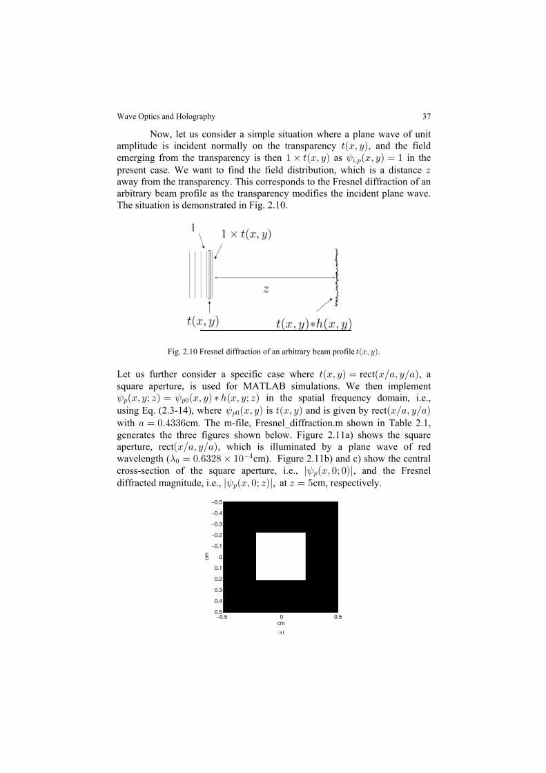
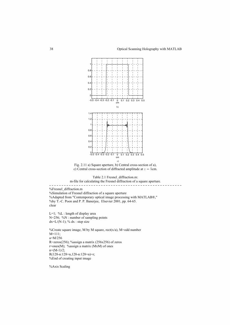
Let us further consider a specific case where >ÐBß CÑ œ rect , aÐBÎ+ß CÎ+Ñsquare aperture, is used for MATLAB simulations. We then implement< <: :!ÐBß Cà DÑ œ ÐBß CÑ ‡ 2ÐBß Cà DÑ in the spatial frequency domain, i.e.,using Eq. (2.3-14), where is given by rect<:!ÐBß CÑ ÐBÎ+ß CÎ+Ñ>ÐBß CÑ and is with cm. + œ !Þ%$$' The m-file, Fresnel_diffraction.m shown in Table 2.1,generates the three figures shown below. Figure 2.11a) shows the squareaperture, rect , which is illuminated by a plane wave of redÐBÎ+ß CÎ+Ñwavelength ( cm). Figure 2.11b) and c) show the central-!

%œ !Þ'$#) ‚ "!cross-section of the square aperture, i.e., , and the Fresnell ÐBß !à !Ñl<:

diffracted magnitude, i.e., , at cm, respectively.l ÐBß !à DÑl D œ &<:

cm

cm

−0.5 0 0.5

−0.5

−0.4

−0.3

−0.2

−0.1

0

0.1

0.2

0.3

0.4

0.5

a)


38

Fig. 2.11 a) Square aperture, b) Central cross-section of a),c) Central cross-section of diffracted amplitude at cm.D œ &

Table 2.1 Fresnel_diffraction.m:m-file for calculating the Fresnel diffraction of a square aperture.

------------------------------------------------------%Fresnel_diffraction.m%Simulation of Fresnel diffraction of a square aperture%Adapted from "Contemporary optical image processing with MATLAB®,"%by T.-C. Poon and P. P. Banerjee, Elsevier 2001, pp. 64-65.clear

L=1; %L : length of display areaN=256; %N : number of sampling pointsdx=L/(N-1); % dx : step size

%Create square image, M by M square, rect(x/a), M=odd numberM=111;a=M/256R=zeros(256); %assign a matrix (256x256) of zerosr=ones(M); %assign a matrix (MxM) of onesn=(M-1)/2;R(128-n:128+n,128-n:128+n)=r;%End of creating input image

%Axis Scaling

−0.5 −0.4 −0.3 −0.2 −0.1 0 0.1 0.2 0.3 0.4 0.5

−0.5 −0.4 −0.3 −0.2 −0.1 0 0.1 0.2 0.3 0.4 0.5

0

0.2

0.4

0.6

0.8

1

cm

cm

b)

0

0.2

0.4

0.6

0.8

1

1.2

1.4

c)


39

for k=1:256 X(k)=1/255*(k-1)-L/2; Y(k)=1/255*(k-1)-L/2;

%Kx=(2*pi*k)/((N-1)*dx) %in our case, N=256, dx=1/255

Kx(k)=(2*pi*(k-1))/((N-1)*dx)-((2*pi*(256-1))/((N-1)*dx))/2; Ky(k)=(2*pi*(k-1))/((N-1)*dx)-((2*pi*(256-1))/((N-1)*dx))/2; end

%Fourier transformation of R

FR=(1/256)^2*fft2(R); FR=fftshift(FR);

%Free space impulse response function% The constant factor exp(-jk0*z) is not calculated%sigma=ko/(2*z)=pi/(wavelength*z)%z=5cm,red light=0.6328*10^-4(cm)sigma=pi/((0.6328*10^-4)*5);

for r=1:256, for c=1:256, %compute free-space impulse response with Gaussian apodization against aliasing h(r,c)=j*(sigma/pi)*exp(-4*200*(X(r).^2+Y(c).^2))*exp(-j*sigma*(X(r).^2+Y(c).^2)); endend

H=(1/256)^2*fft2(h);H=fftshift(H);HR=FR.*H;H=(1/256)^2*fft2(h);H=fftshift(H);HR=FR.*H;

hr=ifft2(HR);hr=(256^2)*hr;hr=fftshift(hr);

%Image of the rectangle objectfigure(1)image(X,Y,255*R);colormap(gray(256));axis squarexlabel('cm')ylabel('cm')

% plot of cross section of squarefigure(2)plot(X+dx/2,R(:,127))grid


40

axis([-0.5 0.5 -0.1 1.2])xlabel('cm')

figure(3)plot(X+dx/2,abs(hr(:,127)))gridaxis([-0.5 0.5 0 max(max(abs(hr)))*1.1])xlabel('cm')------------------------------------------------------

2.4 Ideal Lens, Imaging Systems, Pupil Functionsand Transfer Functions

2.4.1 Ideal Lens and Optical Fourier Transformation

In the previous section, we have discussed light diffraction by apertures. Inthis section, we will discuss the passage of light through an . Anideal lensideal lens is a phase object. When an ideal focusing (or convex) lens hasfocal length , its phase transformation function, , is given by0 > ÐBß CÑ0

> ÐBß CÑ œ Ò4#0

0 exp5

ÐB C ÑÓ! # # , (2.4-1)

where we have assumed that the ideal lens is infinitely thin. For a uniformplane wave incident upon the lens, the wavefront behind the lens is aconverging spherical wave (for > 0) that converges ideally to a point source0( a distance of ) behind the lens. We can see that this is the case whenD œ 0we apply the Eq. (2.3-12)] :Fresnel diffraction formula [see

, (2.4-2)< <: :!ÐBß Cß D œ 0Ñ œ ÐBß CÑ ‡ 2ÐBß Cà D œ 0Ñ

where is now given by <:!ÐBß CÑ " ‚ > ÐBß CÑ0 . The constant, 1, in front of> ÐBß CÑ0 signifies that we have a plane wave (of unit amplitude) incident. Forexample, if we have an incident of the profile given byGaussian beamexp , then expÒ +ÐB C ÑÓ Ò +ÐB C ÑÓ# # # #<:!ÐBß CÑ ‚ will be given by > ÐBß CÑ > ÐBß CÑ0 0. Let us now return to Eq. (2.4-2) where , and by<:!ÐBß CÑ œusing Eq. (2.3-12) we have

<1

: !! w wÐBß Cà 0Ñ œ Ð 45 0Ñ ÐB ß C Ñ

45

# 0exp ( ( >0

‚ B B Ñ C C Ñ .B .Cexpœ 45

#0Ò Ð Ð Ó! # #w w w w

º " ÐB C ÑÓ5( ( exp Ò4

#0! w w# #


41

‚ B C #BB #CC .B .Cexp’ 45

#0Ð Ñ! w w w w w w# # “

œ " BB CC .B .C( ( ’exp ,45

0Ð Ñ! w w w w“

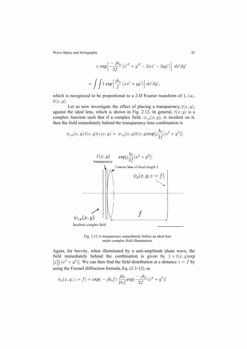
which is recognized to be proportional to a 2-D Fourier transform of , i.e.,"$ÐBß CÑÞ Let us now investigate the effect of placing a transparency, ,>ÐBß CÑagainst the ideal lens, which is shown in Fig. 2.12. In general, is a>ÐBß CÑcomplex function such that if a complex field, , is incident on it,<3ß:ÐBß CÑthen the field immediately behind the transparency-lens combination is

< <3ß: 3ß:! # #ÐBß CÑ >ÐBß CÑ ÐBß CÑ>ÐBß CÑ ÐB C ÑÓÞ

5> ÐBß CÑ œ Ò4

#00 exp

Fig. 2.12 A transparency immediately before an ideal lens under complex field illumination.

Again, for brevity, when illuminated by a unit-amplitude plane wave, thefield immediately behind the combination is given by " ‚ >ÐBß CÑexpÒ4 5 # #!

#0 ÐB C ÑÓ D œ 0. We can then find the field distribution at a distance byusing the Fresnel diffraction formula, Eq. (2.3-12) asß

exp<1

: !!

ÐBß Cà D œ 0Ñ œ Ð 45 0Ñ Ò B C45

# 0exp

45

#0Ð ÑÓ! # #


42

‚ >ÐB ß C Ñ ÐBB CC ÑÓ.B .C5( ( w w w w w w!exp Ò40

œ Ð 45 0Ñ Ò B C45

# 0exp exp!

!

1

45

#0Ð ÑÓ! # #

(2.4-3)‚ >YBCš ›º5Cœ5 CÎ0!

5 œ5 BÎ0B !

,

where and denote the transverse coordinates at . Hence, theB C D œ 0complex field on the focal plane ( is proportional to the FourierD œ 0Ñ

transform of , but has term . Note>ÐBß CÑ Ð ÑÓphase curvature expÒ B C45#0

# #!

that if , i.e., the transparency is completely clear, then we have>ÐBß CÑ œ "< $:ÐBß Cß D œ 0Ñ º ÐBß CÑ, which corresponds to the focusing of a planewave by a lens, as discussed earlier.

Example 2.5 Transparency in front of a Lens

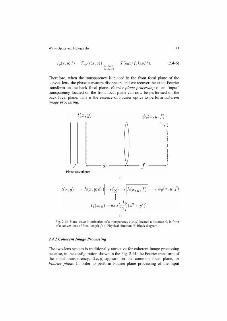
Suppose that a transparency, , is located at a distance, , in front of an>ÐBß CÑ .!ideal convex lens and is illuminated by a plane wave with a unit strengthshown in Fig. 2.13. The physical situation is shown in Fig. 2.13a), which canbe represented by a block diagram given by Fig. 2.13b). According to theblock diagram, we write

, (2.4-4)<: ! 0ÐBß Cà 0Ñ œ ÖÒ>ÐBß CÑ‡2ÐBß Cà . ÑÓ> ÐBß CÑ×‡2ÐBß Cà 0Ñ

which, apart from some constant, can be evaluated to obtain

<1

: !! ! # #ÐBß Cà 0Ñ œ Ò 45 Ð. 0ÑÓ Ò 4 Ð" ÑÐB C ÑÓ

45 5 .

# 0 #0 0exp exp0

0

(2.4-5)‚ ÖYBC º5Cœ5 CÎ0!

5 œ5 BÎ0B !

As in Eq. (2.4-3), note that a phase curvature factor as a function of and B Cagain precedes the Fourier transform, which represents the phase error if onewishes to compute the optical Fourier transformation. However, the phasecurvature vanishes for the special case of . That is, from Eq. (2.4-5). œ 0!

and by disregarding some inessential constant, we now have


ÐBß CÑ

>ÐBß CÑ× .

43

< Y: BC ! !ÐBß Cà 0Ñ œ Ö>ÐBß CÑ× œ XÐ5 BÎ0ß 5 CÎ0Ñº5Cœ5 CÎ0!

5 œ5 BÎ0B !

. (2.4-6)

Therefore, when the transparency is placed in the front focal plane of theconvex lens, the phase curvature disappears and we recover the exact Fouriertransform on the back focal plane. of an input Fourier-plane processingtransparency located on the front focal plane can now be performed on theback focal plane. This is the essence of Fourier optics to perform coherentimage processing.

Fig. 2.13 Plane-wave illumination of a transparency located a distance in front >ÐBß CÑ .!of a convex lens of focal length : a) Physical situation, b) Block diagram.0

2.4.2 Coherent Image Processing

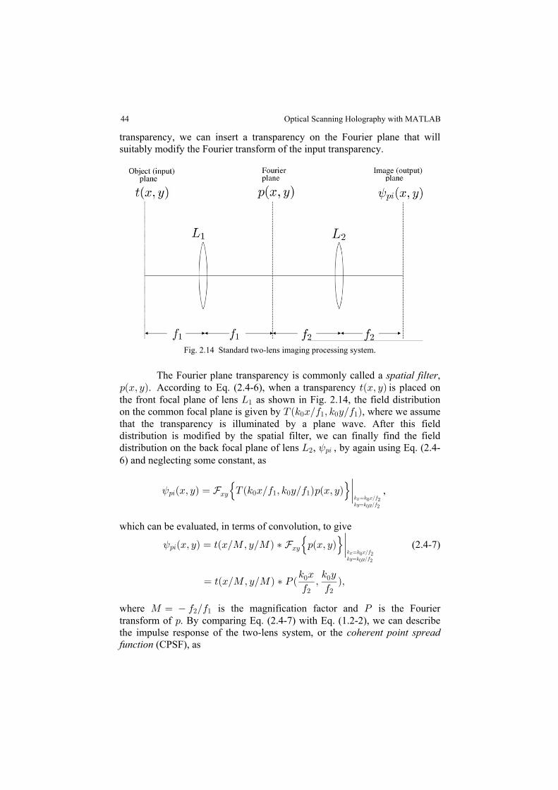
The two-lens system is traditionally attractive for coherent image processingbecause, in the configuration shown in the Fig. 2.14, the Fourier transform ofthe input transparency, , appears on the common focal plane, or>ÐBß CÑFourier plane. In order to perform Fourier-plane processing of the input

“ ”


44

transparency, we can insert a transparency on the Fourier plane that willsuitably modify the Fourier transform of the input transparency.

Fig. 2.14 Standard two-lens imaging processing system.

The Fourier plane transparency is commonly called a ,spatial filter:ÐBß CÑ. According to Eq. (2.4-6), when a transparency is placed on>ÐBß CÑthe front focal plane of lens as shown in Fig. 2.14, the field distributionP"

on the common focal plane is given by , where we assumeXÐ5 BÎ0 ß 5 CÎ0 Ñ! " ! "

that the transparency is illuminated by a plane wave. After this fielddistribution is modified by the spatial filter, we can finally find the fielddistribution on the back focal plane of lens , , by again using Eq. (2.4-P# :3<

6) and neglecting some constant, as

,<:3 ! " ! "ÐBß CÑ œ XÐ5 BÎ0 ß 5 CÎ0 ÑYBCš :ÐBß CÑ›º5Cœ5 CÎ0! #

5 œ5 BÎ0B ! #

which can be evaluated, in terms of convolution, to give

<:3ÐBß CÑ œ >ÐBÎQß CÎQÑ ‡ (2.4-7)YBCš:ÐBß CÑ›º5Cœ5 CÎ0! #

5 œ5 BÎ0B ! #

œ ß Ñß5 5 C

>ÐBÎQß CÎQÑ ‡ TÐB

0 0 ! !

# #

where is the magnification factor and is the FourierQ œ 0 Î0 T# "

transform of :. By comparing Eq. (2.4-7) with Eq. (1.2-2), we can describethe impulse response of the two-lens system, or the coherent point spreadfunction (CPSF), as


45

2 ÐBß CÑ œ œ TÐB

0 0-

# #YBC

! !š:ÐBß CÑ ß Ñ5 5 C›º

5Cœ5 CÎ0! #

5 œ5 BÎ0B ! #

. (2.4-8)

:ÐBß CÑ is often called the of the system. We can see that thepupil functioncoherent PSF is given by the Fourier transform of the pupil function asshown in Eq. (2.4-8). By definition, the corresponding coherent transferfunction is the Fourier transform of the coherent PSF:

L Ð5 ß 5 Ñ œ 2 ÐBß CÑ- B C -YBCš ›

œ TÐ œ :ÐB 0 5

0 0 5 5

0 5YBC

! !š 5 5 C ß Ñ ß ÑÞ

# # ! !

# B # C› (2.4-9)

We observe that is directly proportional to the functionalspatial filteringform of the pupil function in coherent image processing. The complex field on the image plane can then be written as

, (2.4-10)<:3 -ÐBß CÑ º >ÐBÎQß CÎQÑ‡2 ÐBß CÑ

and hence the corresponding isimage intensity

. (2.4-11)M ÐBß CÑ œ l ÐBß CÑl º >ÐBÎQß CÎQÑ ‡ 2 ÐBß CÑl3 :3 -# #< l

2.4.3 Incoherent Image Processing

So far, we have discussed that the illumination of an object is spatiallycoherent - . an example being the use of a laser This means that the complexamplitudes of light falling on all parts of an object vary in unison, meaningthat any two points on an object receive light that has a fixed relative phaseand does not vary with time. On the other hand, an object may be illuminatedwith light having the property that the complex amplitudes on all parts of theobject vary randomly, so that any two points on the object receive light ofillumination is termed . Light from extended sources,spatially incoherentsuch as fluorescent tube lights, is incoherent. As it turns out, a coherentsystem is linear with respect to the complex fields and hence Eqs. (2.4-10)and (2.4-11) hold for . On the other hand, coherent optical systems anincoherent optical system is linear with respect to the intensities. To find theimage intensity, we perform convolution with the given intensity quantitiesas follows:

| | . (2.4-12)M ÐBß CÑ º >ÐBÎQß CÎQÑ ‡ 2 ÐBß CÑl3 -# #l


46

-#

algorithms (e.g., highpass, derivative, etc.), which requires a bipolar PSF[Lohmann and Rhodes (1978)]. As usual, the Fourier transform of an impulse response will give atransfer function known as the of theoptical transfer function (OTF) incoherent imaging system. For this case, it is given by

| , (2.4-13)SXJÐ5 ß 5 Ñ œ Ö 2 ÐBß CÑl × œ L Ð5 ß 5 Ñ Œ L Ð5 ß 5 ÑB C BC - - B C - B C#Y

which can be explicitly written in terms of the coherent transfer function :L-

SXJÐ5 ß 5 Ñ œ L Ð5 ß 5 Ñ L Ð5 5 ß 5 5 Ñ .5 5B C - B C‡ w w w w w w- B C B C B C( ( .

(2.4-14)Note that one of the most important properties of the , which follows aSXJproperty of correlation, is that

| | | 0 0 |. (2.4-15)SXJÐ5 ß 5 Ñ Ÿ SXJÐ ß ÑB C

This property states that the OTF always has a central maximum, whichalways signifies lowpass filtering disregardless of the pupil function used inthe system [Lukosz (1962)].

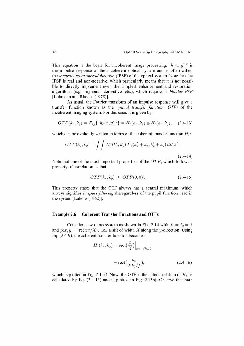
Example 2.6 Coherent Transfer Functions and OTFs

Consider a two-lens system as shown in Fig. 2.14 with 0 œ 0 œ 01 #

and rect , i.e , a slit of width along the -direction. Using:ÐBß CÑ œ ÐBÎ\Ñ Þ \ CEq. (2.4-9), the coherent transfer function becomes

rectL Ð5 ß 5 Ñ œB

\- B C

Bœ05 Î5ˆ ‰¹

B !

œ5

\5 Î0rect , (2.4-16)ˆ ‰B

!

which is plotted in Fig. 2.15a). Now, the OTF is the autocorrelation of asL-

calculated by Eq. (2.4-13) and is plotted in Fig. 2.15b). Observe that both

is |2 Ð ß Ñl B CThis equation is the basis for incoherent image processing.the impulse response of the incoherent optical system and is often called

IPSF is real and non-negative, which particularly means that it is not possi-ble to directly implement even the simplest enhancement and restoration

the intensity point spread functio n (IPSF) of the optical system. Note that the


47

situation perform lowpass filtering of spatial frequencies on an input image.Under incoherent illumination, it is possible to transmit twice the range of

a)

b)Fig. 2.15 a) The coherent transfer function, and b) the OTF

for the pupil function rect .:ÐBß CÑ œ ÐBÎ\Ñ

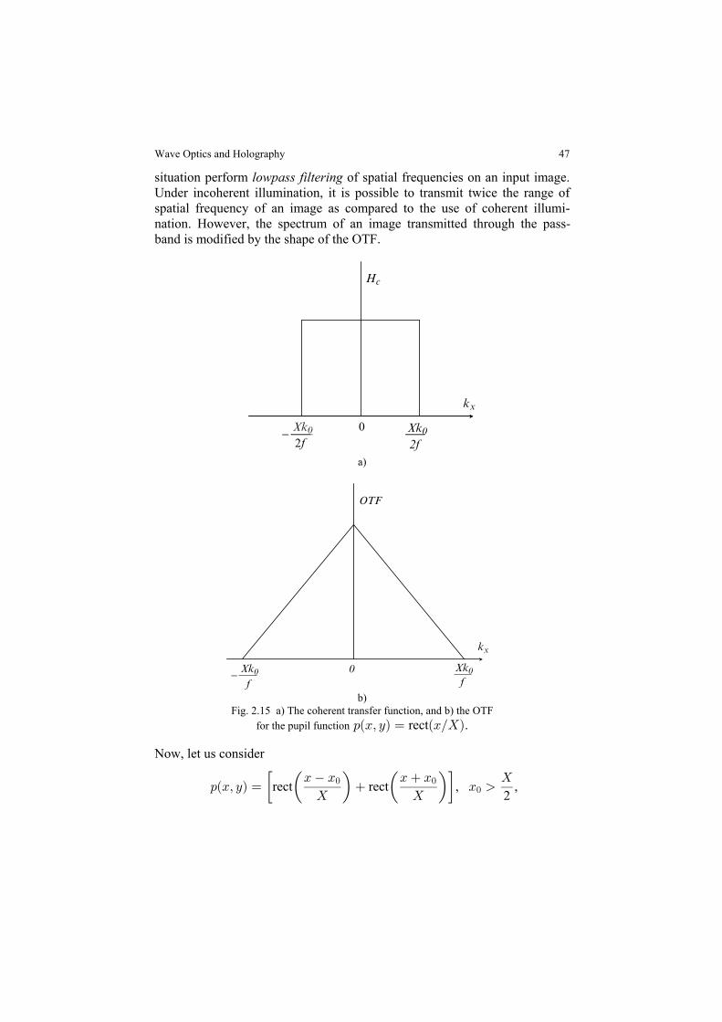
Now, let us consider

:ÐBß CÑ œ B B B B B \

\ \” Œ Œ •rect rect , ,

2! !

!

spatial frequency of an image as compared to the use of coherent illumi-nation. However, the spectrum of an image transmitted through the pass-band is modified by the shape of the OTF.

02f

− Xk0

2fXk0

kx

Hc

0f

Xk0−

OTF

fXk0

kx


48

which is a two-slit object aligned along the -direction. C The coherent transferfunction is

L Ð5 ß 5 Ñ œ- B CBœ05 Î5

” Œ Œ •rect rectB B B B

\ \

! ! ¹B !

œ B B

\ Î \ Î” Œ Œ •rect rect .

5 5 Î0 5 5 Î0

5 0 5 0B ! B !

! !

! !

a)

b)Fig. 2.16 a) The coherent transfer function, and b) the OTF

for the pupil function :ÐBß CÑ œ Ò B B \Ó Ò B B \Órect ( )/ rect ( )/ .! !

We plot L-Ð5 ß 5 ÑB C in Fig. 2.16a) along with the OTF in Fig. 2.16b). Notethat even though it may be possible to achieve withband-pass filtering

fx0k0x0k0

fXk0

fXk0

f−

kx

Hc

0

OTF

f f f

Xk0 Xk0

f

2x0k0 2x0k0− −

kx


49

coherent illumination, incoherent processing always gives rise to inherentlylow-pass characteristics because its point spread function is real and positive[see Eq. (2.4-13)]. A large amount of attention has been focused on devisingmethods to realize band-pass characteristics by using novel incoherent imageprocessing techniques [see, e.g., Lohmann and Rhodes (1978), Stoner (1978),Poon and Korpel (1979), Mait (1987)], where the synthesis of bipolar or evencomplex point spread functions (PSFs) in incoherent optical systems ispossible. Such techniques are called bipolar incoherent image processing.The article by Indebetouw and Poon [1992] provides a comprehensivereview of bipolar incoherent image processing.

2.5 Holography

2.5.1 Fresnel Zone Plate as a Point-Source Hologram

A photograph is a 2-D recording of a 3-D scene. What is actually recorded isthe light intensity at the plane of the photographic recording film - the filmbeing light sensitive only to the intensity variations Hence, the developedÞfilm s amplitude transparency is | | , where is the>ÐBß CÑ º MÐBß CÑ œ < <: :

2

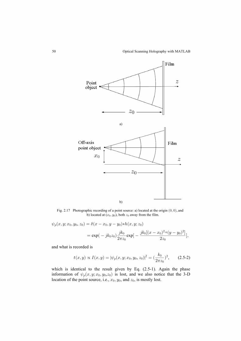
complex field on the film. As a result of this intensity recording, all theinformation on the relative phases of light waves from the original 3-D sceneis lost. This loss of phase information on the light field destroys the 3-Dcharacter of the scene, i.e., we cannot change the perspective of the image inthe photograph by viewing it from a different angle (i.e., ) and we parallaxcannot interpret the depth of the original 3-D scene. As an example, let us take the photographic recording of a pointsource located at the origin, but with a distance of . TheD! away from the filmsituation is shown in Fig. 2.17a). Now, according to Eq. (2.3-15), thecomplex field just before the film is given by

< $: ! !ÐBß Cà D Ñ œ ÐBß CÑ‡2ÐBß Cà D Ñ

exp exp .œ Ð 45 D Ñ Ò Ó45 45 ÐB C Ñ

# D #D! !

! !

! !

# #

1

Hence, the developed film s amplitude transparency is

>ÐBß CÑ º MÐBß CÑ œ ÐBß Cà D Ñ œ Ð| |<: !2 5

# DÑ

!

!

#

1 . (2.5-1)

Note that the phase information of Now, for a<: !ÐBß Cà D Ñ is completely lost.point source located at ( , ), as shown in Fig. 2.17b), tB C! ! he complex fieldjust before the film is given by

’

’


50

a)

b)

! ! !

< $: ! ! ! ! ! !ÐBß Cà B ß C D Ñ œ ÐB B ß C C Ñ‡2ÐBß Cà D Ñ,

exp exp+

œ Ð 45 D Ñ Ò Óß45 45 ÒÐB B Ñ ÐC C Ñ Ó

# D #D! !

! ! ! !

! !

# #

1

and what is recorded is

| |>ÐBß CÑ º MÐBß CÑ œ œ Ð<1

: ! ! !!

!

#ÐBß Cà B ß C D Ñ Ñ5

# D, , (2.5-2)2

which is identical to the result given by Eq. (2.5-1). Again the phaseinformation of , is lost, and we also notice that the 3-D<: ! ! !ÐBß Cà B ß C D Ñlocation of the point source, i.e., , and , is mostly lost.B ß C D! ! !

b) located at (B ß C ), both D away from the film.Fig. 2.17 Photographic recording of a point source: a) located at the origin Ð!ß !Ñ, and


51

Holography is an extraordinary technique that was invented byGabor [1948], where not only the amplitude, but also the phase of a lightfield can be recorded. The word holography combines parts of two Greekwords: , meaning complete, and , meaning to record. Thus,holos grapheinholography means the recording of complete information. Hence, in theholographic process, the film records both the amplitude and phase of a lightfield. The resulting recorded film is called a When a hologram ishologram.properly illuminated, an exact replica of the original 3-D wave field isreconstructed. We shall discuss the of a point objectholographic recordingas an example. Once we know how a single point is recorded, the recordingof a complicated object can be regarded as the recording of a collection ofpoints.

Fig. 2.18 Holographic recording of a point source object.

Figure 2.18 shows a collimated laser which is split into two plane waves andthen recombined by using two mirrors (M) and two beam splitters (BS). Oneplane wave is used to illuminate the pinhole aperture (our point object), andthe other is used to illuminate directly the recording film. The plane wavethat is diffracted by the pinhole aperture generates a diverging sphericalwave. In holography, this diverging wave is known as an . Theobject waveplane wave that directly illuminates the photographic plate is known as areference wave. Let represent the field distribution of the object wave on<othe plane of the recording film, and similarly, let represent the field<r distribution of the reference wave on the plane of the recording film. Thefilm now records the interference of the reference wave and the object wave,i.e., what is recorded is given by , provided that the referencel l< <r o

#

wave and the object wave are mutually coherent over the film. The

“ ”“ ” “ ”

“ ”


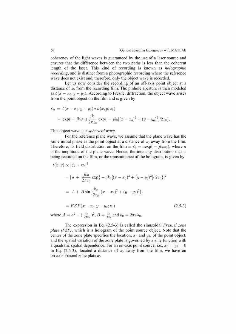
52

coherency of the light waves is guaranteed by the use of a laser source andensures that the difference between the two paths is less than the coherentlength of the laser. This kind of recording is known as holographicrecording, and is distinct from a photographic recording where the referencewave does not exist and, therefore, only the object wave is recorded. Let us now consider the recording of an off-axis point object at adistance of from the recording film. The pinhole aperture is then modeledD!as . According to Fresnel diffraction, the object wave arises$a bB B ß C C! !

from the point object on the film and is given by

< $o œ B B ß C Ca b! ! ‡ 2ÐBß Cà D Ñ!

exp / . 2

œ D Ö 45 ÒÐB B Ñ ÐC C Ñ Ó #D ×45

DexpÐ 45 Ñ! ! ! !

!

!! !1

2 2

This object wave is a .spherical wave For the reference plane wave, we assume that the plane wave has thesame initial phase as the point object at a distance of away from the film.D!Therefore, its field distribution on the film is , where <r œ + D +expÐ 45 Ñ! !

is the amplitude of the plane wave. Hence, the intensity distribution that isbeing recorded on the film, or the transmittance of the hologram, is given by

>ÐBß CÑ º l l< <r o#

exp / 2

œ l + Ö 45 ÒÐB B Ñ ÐC C Ñ Ó #D ×l45

D!

!! !! !1

2 2 2

œ E F Ö ÒÐB B Ñ ÐC C Ñ Ó×5

D

2sin !

!! !

2 2

œ J^TÐB B ß C C à D Ñ! ! ! (2.5-3)

where ( ) , and .E œ + F œ 5 œ # Î# 5 5D D ! !! !

! !22

1 11 -

The expression in Eq. (2.5-3) is called the sinusoidal Fresnel zoneplate (FZP) , which is a hologram of the point source object. Note that thecenter of the zone plate specifies the location, and , of the point object,B C! !

and the spatial variation of the zone plate is governed by a sine function witha quadratic spatial dependence. For an on-axis point source, i.e., B œ C œ !! !

!

on-axis Fresnel zone plate asin Eq. (2.5-3), located a distance of D away from the film, we have an


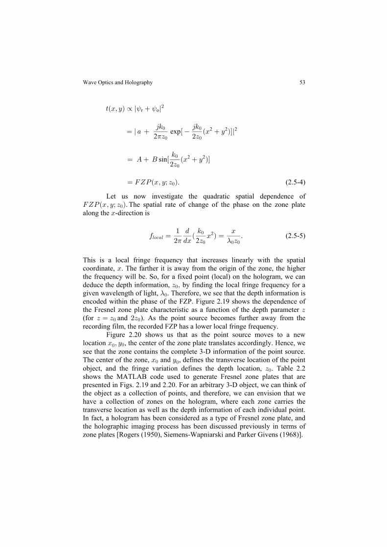
53

>ÐBß CÑ º l l< <r o#

exp2

œ l + Ò ÐB C ÑÓl45 45

D #D! !

! !12 2 2

œ E F Ò ÐB C ÑÓ5

#D sin !

!

2 2

œ J^TÐBß Cà D Ñ! . (2.5-4)

Let us now investigate the quadratic spatial dependence ofJ^TÐBß Cà D Ñ! . The spatial rate of change of the phase on the zone platealong the -direction isB

0 œ Ð B Ñ œ" . 5 B

# .B D D69-+6

!

! ! !

#

1 -2. (2.5-5)

This is a local fringe frequency that increases linearly with the spatialcoordinate, . The farther it is away from the origin of the zone, the higherBthe frequency will be. So, for a fixed point (local) on the hologram, we candeduce the depth information, by finding the local fringe frequency for aD ß!given wavelength of light, . Therefore, we see that the depth information is-!

encoded within the phase of the FZP. Figure 2.19 shows the dependence ofthe Fresnel zone plate characteristic as a function of the depth parameter D(for and ). As the point source becomes further away from theD œ D #D! !

recording film, the recorded FZP has a lower local fringe frequency. Figure 2.20 shows us that as the point source moves to a newlocation , the center of the zone plate translates accordingly. Hence, weB ß C! !

see that the zone contains the complete 3-D information of the point source.The center of the zone, and , defines the transverse location of the pointB C! !

object, and the fringe variation defines the depth location, . Table 2.2D!shows the MATLAB code used to generate Fresnel zone plates that arepresented in Figs. 2.19 and 2.20. For an arbitrary 3-D object, we can think ofthe object as a collection of points, and therefore, we can envision that wehave a collection of zones on the hologram, where each zone carries thetransverse location as well as the depth information of each individual point.In fact, a hologram has been considered as a type of Fresnel zone plate, andthe holographic imaging process has been discussed previously in terms ofzone plates [Rogers (1950), Siemens-Wapniarski and Parker Givens (1968)].


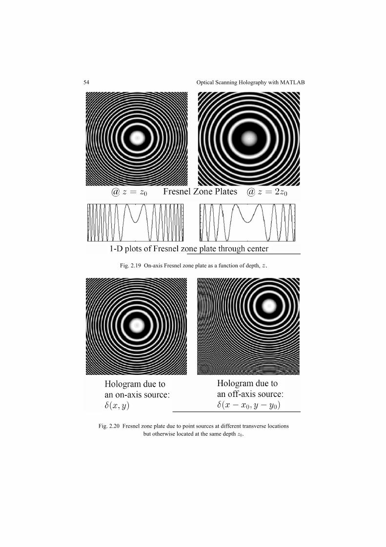
54

Fig. 2.19 On-axis Fresnel zone plate as a function of depth, D.

Fig. 2.20 Fresnel zone plate due to point sources at different transverse locationsbut otherwise located at the same depth D!.


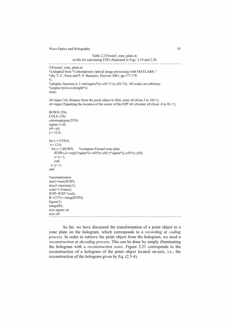
55

Table 2.2 Fresnel_zone_plate.m:m-file for calculating FZPs illustrated in Figs. 2.19 and 2.20.

------------------------------------------------------%Fresnel_zone_plate.m%Adapted from "Contemporary optical image processing with MATLAB®,"%by T.-C. Poon and P. P. Banerjee, Elsevier 2001, pp.177-178.%%display function is 1+sin(sigma*((x-x0)^2+(y-y0)^2)). All scales are arbitrary.%sigma=pi/(wavelength*z)clear;

z0=input ('z0, distance from the point object to film, enter z0 (from 2 to 10)=');x0=input ('Inputting the location of the center of the FZP x0=y0,enter x0 (from -8 to 8) =');

ROWS=256;COLS=256;colormap(gray(255))sigma=1/z0;y0=-x0;y=-12.8;

for r=1:COLS, x=-12.8; for c=1:ROWS, %compute Fresnel zone plate fFZP(r,c)=exp(j*sigma*(x-x0)*(x-x0)+j*sigma*(y-y0)*(y-y0)); x=x+.1; end y=y+.1;end

%normalizationmax1=max(fFZP);max2=max(max1);scale=1.0/max2;fFZP=fFZP.*scale;R=127*(1+imag(fFZP));figure(1)image(R);axis square onaxis off------------------------------------------------------

So far, we have discussed the transformation of a point object to azone plate on the hologram, which corresponds to a or recording codingprocess. In order to retrieve the point object from the hologram, we need areconstruction decoding process or . This can be done by simply illuminatingthe hologram with a . Figure 2.21 corresponds to thereconstruction wavereconstruction of a hologram of the point object located on-axis, i.e., thereconstruction of the hologram given by Eq. (2.5-4).


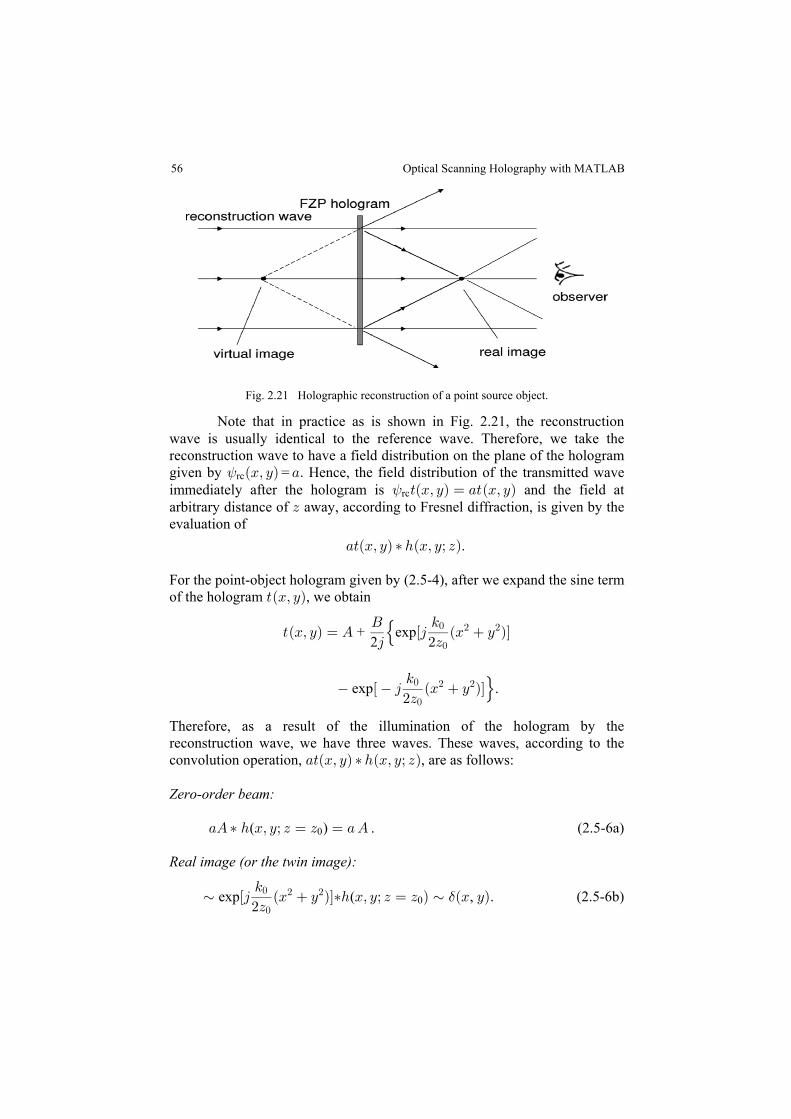
56

Fig. 2.21 Holographic reconstruction of a point source object.

Note that in practice as is shown in Fig. 2.21, the reconstructionwave is usually identical to the reference wave. Therefore, we take thereconstruction wave to have a field distribution on the plane of the hologramgiven by = Hence, the field distribution of the transmitted wave<rca bBß C +Þimmediately after the hologram is and the field at<rc> Bß C œ +> Bß Ca b a barbitrary distance of away, according to Fresnel diffraction, is given by theDevaluation of . +> Bß C ‡ 2 Bß Cà Da b a bFor the point-object hologram given by (2.5-4), after we expand the sine termof the hologram , we obtain> Bß Ca b

>ÐBß CÑ œ E Ò4 ÐB C ÑÓF 5

4 #D + exp

2š !

!

# #

exp . Ò 4 ÐB C ÑÓ5

#D!

!

# # ›Therefore, as a result of the illumination of the hologram by thereconstruction wave, we have three waves. These waves, according to theconvolution operation, , are as follows:+> Bß C ‡ 2 Bß Cà Da b a bZero-order beam:

( ) . (2.5-6a)+E‡ 2 Bß Cà D œ D œ +E0

Real image (or the twin image):

μ Ò4 ÐB C ÑÓ‡2 Bß Cà D œ D Ñ μ ÐB CÑ5

#Dexp ( , . (2.5-6b)!

!

# #0 $


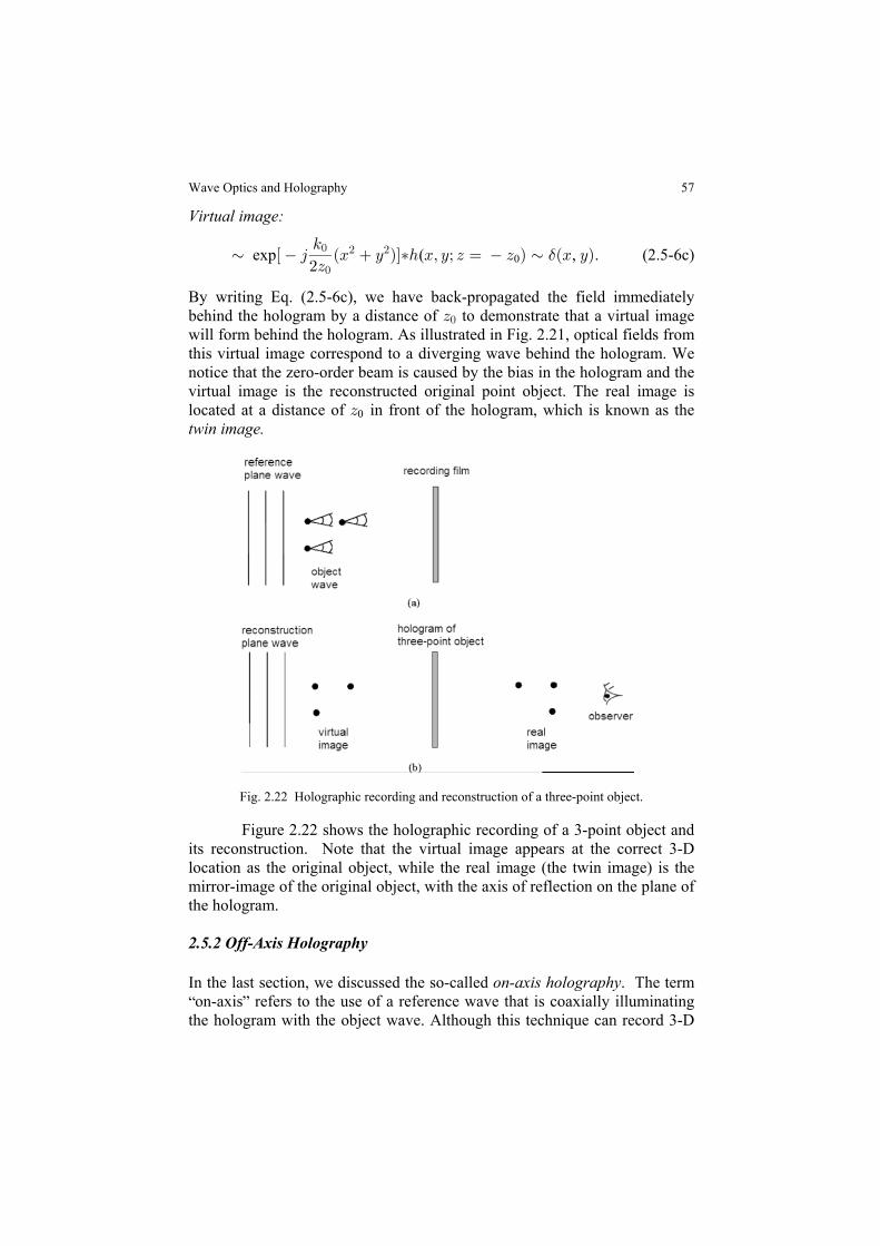
57

Virtual image:

μ Ò 4 ÐB C ÑÓ‡2 Bß Cà D œ D Ñ μ ÐB CÑ5

#D exp ( , . (2.5-6c)!

!

# #0 $

By writing Eq. (2.5-6c), we have back-propagated the field immediatelybehind the hologram by a distance of to demonstrate that a virtual imageD!will form behind the hologram. As illustrated in Fig. 2.21, optical fields fromthis virtual image correspond to a diverging wave behind the hologram. Wenotice that the zero-order beam is caused by the bias in the hologram and thevirtual image is the reconstructed original point object. The real image islocated at a distance of in front of the hologram, which is known as theD0twin image.

Fig. 2.22 Holographic recording and reconstruction of a three-point object.

Figure 2.22 shows the holographic recording of a 3-point object andits reconstruction. Note that the virtual image appears at the correct 3-Dlocation as the original object, while the real image (the twin image) is themirror-image of the original object, with the axis of reflection on the plane ofthe hologram.

2.5.2 Off-Axis Holography

In the last section, we discussed the so-called . The termon-axis holographyon-axis refers to the use of a reference wave that is coaxially illuminating

the hologram with the object wave. Although this technique can record 3-D“ ”


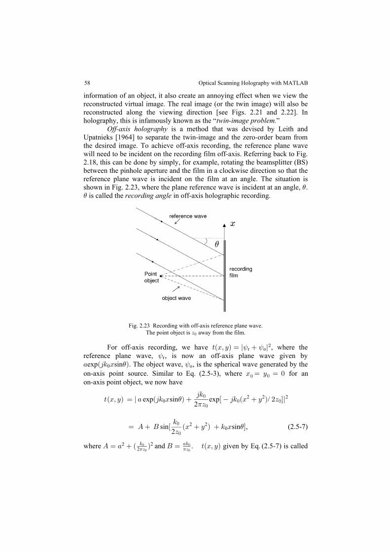
58

information of an object, it also create an annoying effect when we view thereconstructed virtual image. The real image (or the twin image) will also bereconstructed along the viewing direction [see Figs. 2.21 and 2.22]. Inholography, this is infamously known as the twin-image problem. Off-axis holography is a method that was devised by Leith and

the desired image. To achieve off-axis recording, the reference plane wavewill need to be incident on the recording film off-axis. Referring back to Fig.2.18, this can be done by simply, for example, rotating the beamsplitter (BS)between the pinhole aperture and the film in a clockwise direction so that thereference plane wave is incident on the film at an angle. The situation isshown in Fig. 2.23, where the plane reference wave is incident at an angle, .)) is called the in off-axis holographic recording.recording angle

Fig. 2.23 Recording with off-axis reference plane wave.The point object is away from the film.D!

For off-axis recording, we have , where the>ÐBß CÑ œ l l< <r o#

reference plane wave, , is now an off-axis plane wave given by<r+ Ð45 B Ñexp sin0 o) <. The object wave, , is the spherical wave generated by the

! !

>ÐBß CÑ œ l + Ð45 B Ñ Ò 45 ÐB C Ñ #D Ól45

Dexp sin0

2 2 2)1

!

!! !2

exp /

, (2.5-7)2

œ E F Ò ÐB C Ñ 5 B Ó5

Dsin sin!

!

2 20 )

where and . given by Eq. (2.5-7) is calledE œ + Ð Ñ F œ > Bß C# 5 +5D D! !

! !22

1 1a b

“ ”

on-axis point object, we now haveon-axis point source. Similar to Eq. (2.5-3), where B œ C œ ! for an


Upatnieks [1964] to separate the twin-image and the zero-order beam from

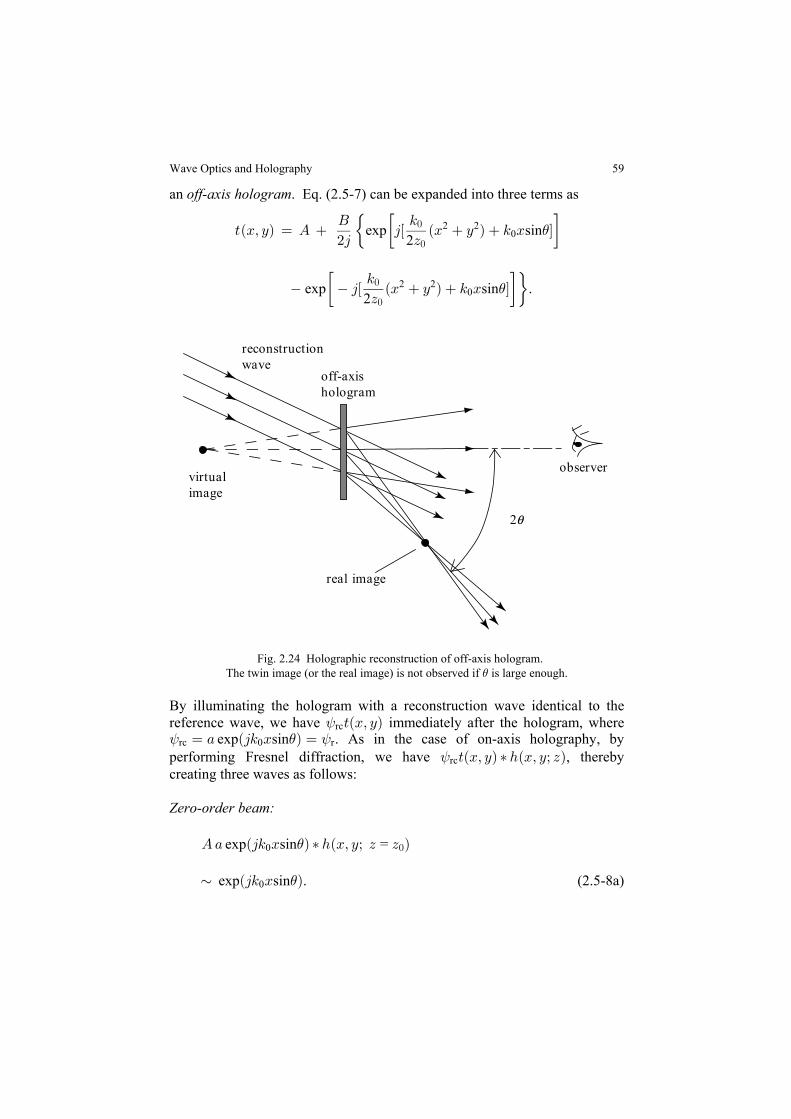
59

an . Eq. (2.5-7) can be expanded into three terms asoff-axis hologram

>ÐBß CÑ œ E 4Ò ÐB C Ñ 5 B ÓF 5

#4 Dœ ” •exp sin!

!22 2

0 )

.2

4Ò ÐB C Ñ 5 B Ó5

Dexp sin” •!

!

2 20 )

Fig. 2.24 Holographic reconstruction of off-axis hologram.The twin image (or the real image) is not observed if is large enough.)

By illuminating the hologram with a reconstruction wave identical to thereference wave, we have immediately after the hologram, where<rc> Bß Ca b< ) <rc 0 rœ + Ð45 B Ñ œexp sin . As in the case of on-axis holography, byperforming Fresnel diffraction, we have , thereby<rc> Bß C ‡ 2 Bß Cà Da b a bcreating three waves as follows:

Zero-order beam:

E+ Ð45 B Ñ ‡ 2ÐBß Cà D D Ñexp sin0 ) = !

μ Ð45 B Ñexp sin0 ) . (2.5-8a)

virtualimage

real image

off-axishologram

reconstructionwave

observer

2q


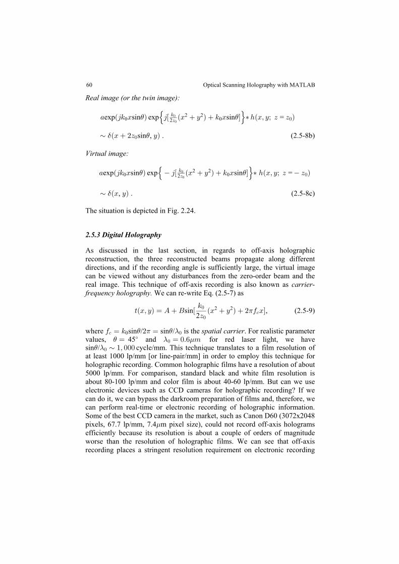
60

Real image (or the twin image):

+ Ð45 B Ñ 4Ò ÐB C Ñ 5 B Ó ‡ 2ÐBß Cà D D Ñexp sin exp sin0 022 2) )š ›5

D !!

! =

μ ÐB #D CÑ$ )!sin , . (2.5-8b)

Virtual image:

+ Ð45 B Ñ 4Ò ÐB C Ñ 5 B Ó ‡ 2ÐBß Cà D D Ñexp sin exp sin0 022 2) )š ›5

D !!

! =

μ ÐB CÑ Þ$ , (2.5-8c)

The situation is depicted in Fig. 2.24.

2.5.3 Digital Holography

As discussed in the last section, in regards to off-axis holographicreconstruction, the three reconstructed beams propagate along differentdirections, and if the recording angle is sufficiently large, the virtual imagecan be viewed without any disturbances from the zero-order beam and thereal image. This technique of off-axis recording is also known as carrier-frequency holography. We can re-write Eq. (2.5-7) as

>ÐBß CÑ œ E F Ò ÐB C Ñ # 0 BÓ5

Dsin !

!-2

, (2.5-9)2 2 1

where / / is the . For realistic parameter0 œ 5 # œ- !0sin sin) 1 ) - spatial carriervalues, 45 and for red laser light, we have) - .œ œ !Þ' 7‰

!

sin) -/ cycle/mm. This technique translates to a film resolution of! μ "ß !!!at least 1000 lp/mm [or line-pair/mm] in order to employ this technique forholographic recording. Common holographic films have a resolution of about5000 lp/mm. For comparison, standard black and white film resolution isabout 80-100 lp/mm and color film is about 40-60 lp/mm. But can we useelectronic devices such as CCD cameras for holographic recording? If wecan do it, we can bypass the darkroom preparation of films and, therefore, wecan perform real-time or electronic recording of holographic information.Some of the best CCD camera in the market, such as Canon D60 (3072x2048pixels, 67.7 lp/mm, 7.4 m pixel size), could not record off-axis holograms.efficiently because its resolution is about a couple of orders of magnitudeworse than the resolution of holographic films. We can see that off-axisrecording places a stringent resolution requirement on electronic recording


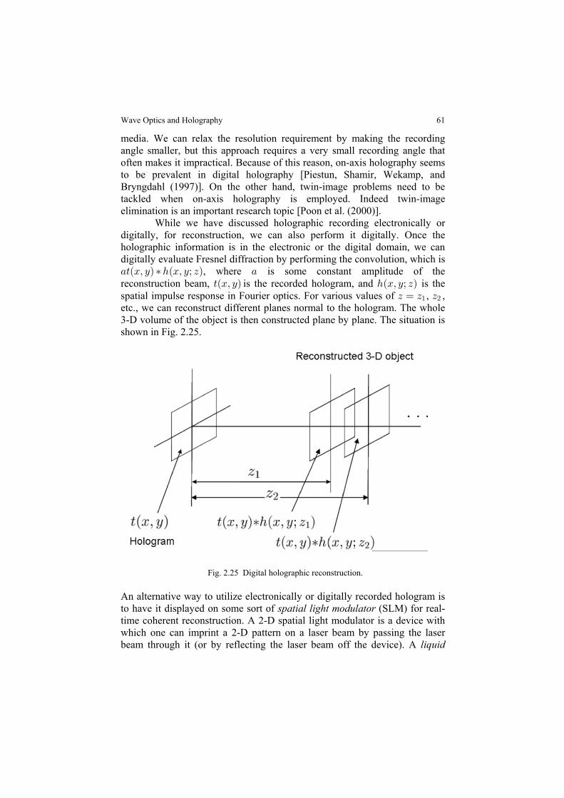
61

media. We can relax the resolution requirement by making the recordingangle smaller, but this approach requires a very small recording angle thatoften makes it impractical. Because of this reason, on-axis holography seemsto be prevalent in digital holography [Piestun, Shamir, Wekamp, andBryngdahl (1997)]. On the other hand, twin-image problems need to betackled when on-axis holography is employed. Indeed twin-imageelimination is an important research topic [Poon et al. (2000)]. While we have discussed holographic recording electronically ordigitally, for reconstruction, we can also perform it digitally. Once theholographic information is in the electronic or the digital domain, we candigitally evaluate Fresnel diffraction by performing the convolution, which is+> Bß C ‡ 2 Bß Cà D +a b a b, where is some constant amplitude of thereconstruction beam, is the recorded hologram, and is the>ÐBß CÑ 2ÐBß Cà DÑspatial impulse response in Fourier optics. For various values of , ,D œ D D" #

etc., we can reconstruct different planes normal to the hologram. The whole3-D volume of the object is then constructed plane by plane. The situation isshown in Fig. 2.25.

Fig. 2.25 Digital holographic reconstruction.

An alternative way to utilize electronically or digitally recorded hologram isto have it displayed on some sort of (SLM) for real-spatial light modulator time coherent reconstruction. A 2-D spatial light modulator is a device withwhich one can imprint a 2-D pattern on a laser beam by passing the laserbeam through it (or by reflecting the laser beam off the device). A liquid


62

crystal television (LCTV) (upon suitably modification) is a good example ofspatial light modulators. In fact, we can think of a spatial light modulator as areal-time transparency because one can update 2-D images or hologramsupon the spatial light modulator in real time without developing films into

All in all, in this section we mention electronic or digital recordingand manipulation of holographic information. This type of research iscommonly known as (or ) . The reader may finddigital electronic holographya pioneering contribution in the work of Goodman and Lawrence [1967].Ever since, digital holography has become a practical tool with an increasingnumber of applications [Schnars and Juptner (2002)]. Most recently, anedited book on the subject organizes a collection of key chapters that coversdigital holography and 3-D display techniques so as to provide the readerwith the state-of-the-art developments in these important areas around theworld [Poon (2006)]. Starting in the next chapter, we will discuss a uniqueelectronic holographic recording technique called optical scanningholography.

References

2.1 Banerjee, P.P. and T.-C. Poon (1991). Irwin, Illinois.Principles of Applied Optics.2.2 Gabor, D. (1948). A new microscopic principle, Nature2.3 Goodman, J. W. and R.W. Lawrence (1967). Digital image formation from

electronically detected holograms,2.4 Goodman, J. W. (2005). . 3rd. ed., Roberts andIntroduction to Fourier Optics

Company Publishers, Englewood, Colorado.2.5 Indebetouw, G. and T.-C. Poon (1992). Novel approaches of incoherent image

processing with emphasis on scanning methods, 31, 2159–Optical Engineering2167.

2.6 E. N. Leith, E.N and J. Upatnieks (1962). Reconstructed wavefronts andcommunication theory, 52, 1123–1130.Journal of the Optical Society of America

2.7 functions, 17, 1141-1150.Applied Optics

2.8 Lukosz, W. (1962). Properties of linear low pass filters for non-negative signals,Journal of the Optical Society of America 52, 827-829.

2.9 Mait, J. N. (1987). Pupil-function design for complex incoherent spatial filtering,Journal of the Optical Society of America A 4, 1185- 1193.

2.10 Piestun R., J. Shamir, B. Wekamp, and O. Bryngdahl (1997). On-axis computer-generated holograms for three-dimensional display, 22, 922-924.Optics Letters

2.11 Poon, T.-C. and A. Korpel (1979). Optical transfer function of an acousto-opticheterodyning image processor, 4, 317-319.Optics Letters

2.12 Poon, T.-C., T. Kim, G. Indebetouw, B. W. Schilling, M. H. Wu, K. Shinoda, andY. Suzuki (2000). Twin-image elimination experiments for three-dimensionalimages in optical scanning holography, 25, 215-217.Optics Letters

transparencies. Again, off-axis holographic recording places stringent reso-lution requirement on SLMs and we will come back to this later when dis-cussing 3-D display applications in Chapter 4.

“ ”“

”

“”

“”

”“ ”

“ ”

“”

“”

“”

Applied Physics Letters 11, 77-79.

Lohmann A.W. and W. T. Rhodes (1978). “Two-pupil synthesis of optical transfer


63

2.13 Poon T.-C. and P. P. Banerjee (2001). Contemporary Optical Image Processingwith MATLAB . ® Elsevier, Oxford, UK.

2.14 Poon, T.-C., ed., (2006). Digital Holography and Three-Dimensional Display:

2.15 Rogers, G.L. (1950). The black and white holograms, 166, 1027.Nature 2.16 Siemens-Wapniarski, W.J. and M. Parker Givens (1968). The experimental

production of synthetic holograms, 7, 535-538. Applied Optics2.17 Stoner, W. (1978). Incoherent optical processing via spatially offset pupil masks,

Applied Optics 17, 2454-2466.2.18 Schnars, U. and W. P. O. Juptner (2002). Digital recording and numerical

reconstruction of holograms, 13, R85–R101.Meas. Sci. Technol.

“ ”“

”“ ”

“”


Principles and Applications. . Springer, New York, USA.

Chapter 3

Optical Scanning Holography: Principles

Optical scanning holography (OSH) is a form of electronic (or digital)

single 2-D optical scan. OSH was first implicated by Poon and Korpel whenthey investigated bipolar incoherent image processing on their acousto-opticheterodyning image processor [1979]. The original idea is later formulatedand becomes known as [Poon (1985)]. The firstscanning holographyexperimental results were then demonstrated and the technique waseventually called optical scanning holography in order to emphasize thenovel fact that holographic recording can be achieved by active opticalscanning [Duncan and Poon (1992)]. Thus far, applications of OSH includescanning holographic microscopy [(Poon, Doh, Schilling, Wu, Shinoda, andSuzuki (1995)], 3-D image recognition [(Poon and Kim (1999)], 3-D opticalremote sensing [Kim and Poon (1999)], 3-D TV and display [Poon (2002a)],and 3-D cryptography [Poon, Kim, and Doh (2003)]. Scanning holographicmicroscopy is, by far, the most developed technique that utilizes OSH.Unlike any other holographic microscopes, scanning holographic microscopehas a unique property that allows it to take the holographic information offluorescent specimens in three dimensions. Recently, scientists have beenable to achieve better than one-micron resolution in holographic fluorescencemicroscopy [Indebetouw and Zhong (2006)]. While in chapters 1 and 2, wehave covered the necessary backgrounds in mathematics and optics to betterunderstand OSH, in this chapter, we discuss the basic principles of OSH. Inchapter 4, we will then discuss some of the previously mentionedapplications of OSH in detail. Finally in chapter 5, we will discuss somerecent advances in OSH.

3.1 Principle of Optical Scanning

Optical scanning holography involves active and optical scanning opticalheterodyning. In this section, we will discuss the basics of optical scanning.An optical scanner or optical processor scans out a transparency, i.e.,information, with an optical beam by moving either the beam or thetransparency. A photodetector accepts all light and gives an electrical output

holography. It is a unique, real-time technique where holographic infor-mation of a three-dimensional (3-D) object can be acquired by using a

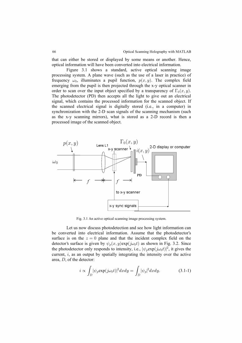
that can either be stored or displayed by some means or another. Hence,optical information will have been converted into electrical information. Figure 3.1 shows a standard, active optical scanning imageprocessing system. A plane wave (such as the use of a laser in practice) offrequency , illuminates a pupil function, The complex field=! :ÐBß CÑÞemerging from the pupil is then projected through the x-y optical scanner inorder to scan over the input object specified by a transparency of .>!ÐBß CÑThe photodetector (PD) then accepts all the light to give out an electricalsignal, which contains the processed information for the scanned object. Ifthe scanned electrical signal is digitally stored (i.e., in a computer) insynchronization with the 2-D scan signals of the scanning mechanism (suchas the x-y scanning mirrors), what is stored as a 2-D record is then aprocessed image of the scanned object.

Fig. 3.1 An active optical scanning image processing system.

Let us now discuss photodetection and see how light information canbe converted into electrical information. Assume that the photodetector ssurface is on the plane and that the incident complex field on theD œ !detector s surface is given by exp as shown in Fig. 3.2< =: !ÐBß CÑ Ð4 >Ñ Þ Sincethe photodetector only responds to intensity, i.e., | , it gives thel<:

#expÐ4 >Ñ=!

current, , as an output by spatially integrating the intensity over the active3area, , of the detector:H

3 º l Ð4 >Ñ .B.C œ l .B.C( (H H

: ! :# #< = <exp | | . (3.1-1)

66

’

’


67

For example, if the incident field is a plane wave of amplitude , i.e.,E<: œ E, the current output is given by

3 º lE .B.C œ E H(H

# #| , (3.1-2)

which is a constant. However, take for instance that if the light has beenintensity-modulated, i.e., | | , where is the modulating signal,<:

# œ 7Ð>Ñ 7Ð>Ñthe current will then give an output that varies with the modulation. This isuseful for laser communications systems [Pratt (1969)]. Note that since exp , the output< < 9: :ÐBß CÑ œ l ÐBß CÑl Ò4 ÐBß CÑÓcurrent can only contain the magnitude information, i.e., , and the phasel l<:

information is completely lost. This type of photodetection is known asoptical direct detection optical incoherent detection(or ).

Figure 3.2 Optical direct detection.

Once we comprehend photodetection, we can return to Fig. 3.1 to calculatethe current output given after scanning the transparency, . Instead of>!ÐBß CÑmodeling the transparency that is being scanned by an optical beam, asshown by Fig. 3.3, we assume that the transparency, , is moving through>!

the optical beam. In Fig. 3.3, the plane of the photodetector is on the B Cw w

plane and the optical scanning beam specified by a complex field, , is,ÐB ß C Ñw w

stationary at the origin of the plane. By scanning or sampling weB Cw w

mean that successive points ( , , in transparency coordinates) of areB C >!

brought into coincidence with the center ( , ) of the optical beam inB C œ !w w

the plane.B Cw w

Fig. 3.3 Scanning situation.


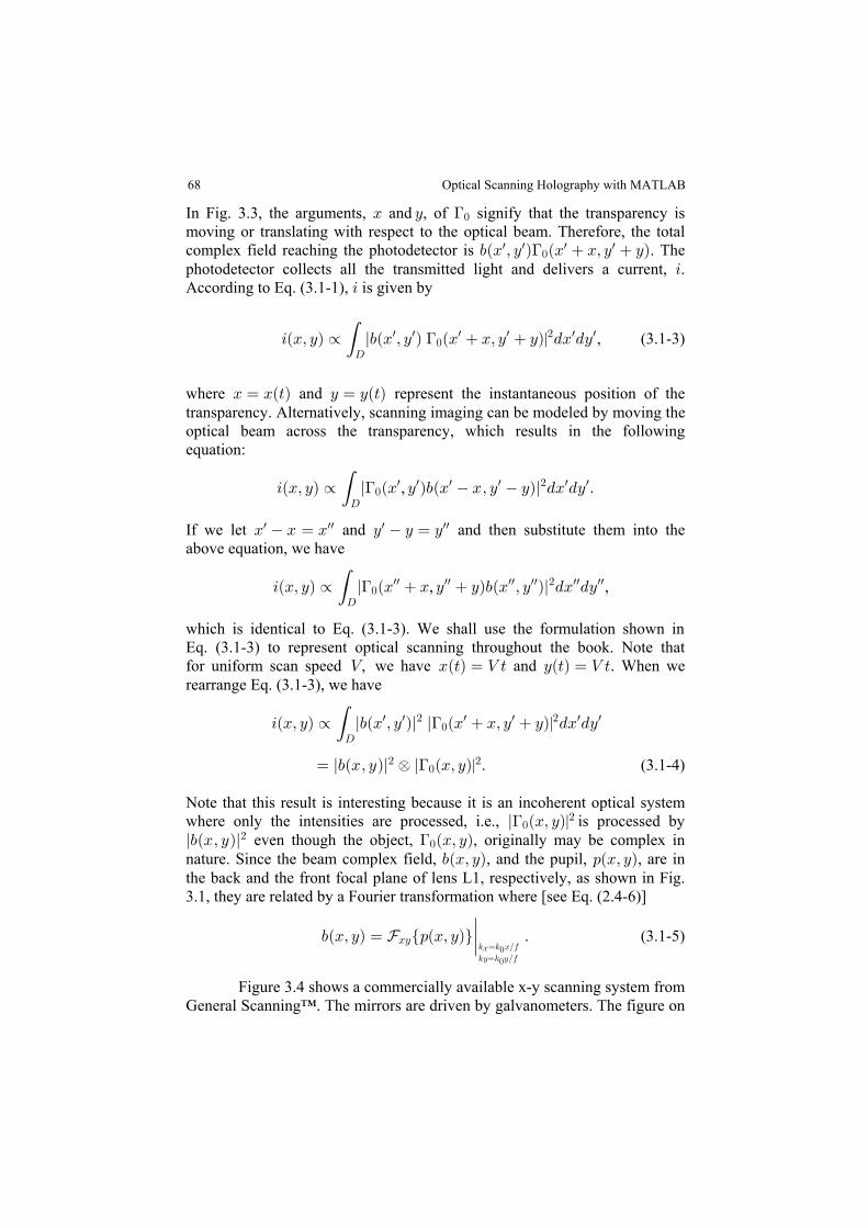
68

In Fig. 3.3, the arguments, and , of signify that the transparency isB C >!

moving or translating with respect to the optical beam. Therefore, the totalcomplex field reaching the photodetector is . The,ÐB ß C Ñw w >!

w wÐB Bß C CÑphotodetector collects all the transmitted light and delivers a current, .3According to Eq. (3.1-1), is given by3

3ÐBß CÑ º l,ÐB ß C Ñ B .C(H

w w w w | (3.1-3)>!w w #ÐB Bß C CÑ . ,

where and represent the instantaneous position of theB œ BÐ>Ñ C œ CÐ>Ñtransparency. Alternatively, scanning imaging can be modeled by moving theoptical beam across the transparency, which results in the followingequation:

,3ÐBß CÑ º ,ÐB Bß C CÑl B .C Þ(H

w w # w wl ÐB C Ñ .>!w w

If we let B B œ B C C œ Cw ww w ww and and then substitute them into theabove equation, we have

3ÐBß CÑ º ,ÐB ß C Ñl B .C(H

ww ww # ww wwl ÐB B C CÑ .>!ww ww, ,

3ÐBß CÑ º l,ÐB ß C Ñl B .C(H

w w # w w |l ÐB Bß C CÑ .>!w w #

| . (3.1-4)œ l ÐBß CÑl,ÐBß CÑl Œ# >!#

Note that this result is interesting because it is an incoherent optical systemwhere only the intensities are processed, i.e., | is processed byl ÐBß CÑ>!

#

l,ÐBß CÑl# even though the object, originally may be complex in>!ÐBß CÑ, nature. Since the beam complex field, , and the pupil, , are in,ÐBß CÑ :ÐBß CÑthe back and the front focal plane of lens L1, respectively, as shown in Fig.3.1, they are related by a Fourier transformation where [see Eq. (2.4-6)]

. (3.1-5),ÐBß CÑ œ Ö:ÐBß CÑ×YBC º5Cœ5 CÎ0!

5 œ5 BÎ0B !

Figure 3.4 shows a commercially available x-y scanning system fromGeneral Scanning™. The mirrors are driven by galvanometers. The figure on

rearrange Eq. (3.1-3), we haveÐ>Ñ œ Z > and CÐ>Ñ œ Z >. When we

which is identical to Eq. (3.1-3). We shall use the formulation shown in Eq. (3.1-3) to represent optical scanning throughout the book. Note thatfor uniform scan speed Z B, we have


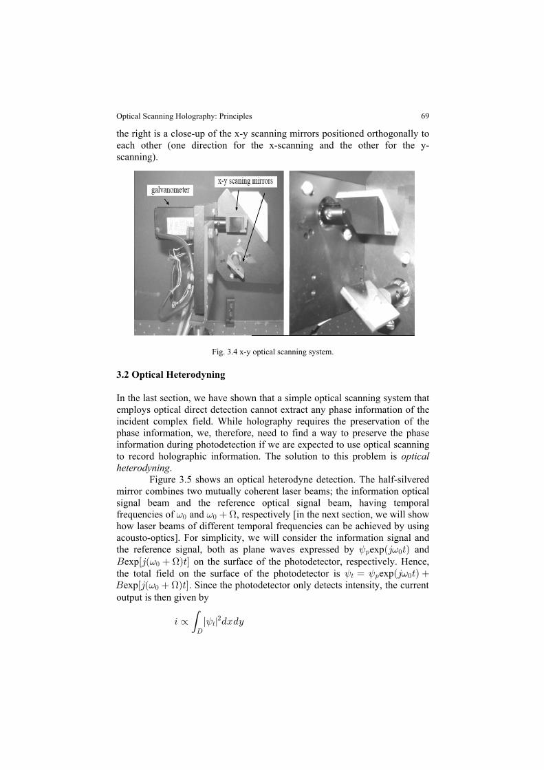
69

the right is a close-up of the x-y scanning mirrors positioned orthogonally toeach other (one direction for the x-scanning and the other for the y-scanning).

Fig. 3.4 x-y optical scanning system.

3.2 Optical Heterodyning

In the last section, we have shown that a simple optical scanning system thatemploys optical direct detection cannot extract any phase information of theincident complex field. While holography requires the preservation of thephase information, we, therefore, need to find a way to preserve the phaseinformation during photodetection if we are expected to use optical scanningto record holographic information. The solution to this problem is opticalheterodyning. Figure 3.5 shows an optical heterodyne detection. The half-silveredmirror combines two mutually coherent laser beams; the information opticalsignal beam and the reference optical signal beam, having temporalfrequencies of and , respectively [in the next section, we will show= = H! ! how laser beams of different temporal frequencies can be achieved by usingacousto-optics]. For simplicity, we will consider the information signal andthe reference signal, both as plane waves expressed by exp and< =: !Ð4 >ÑF Ò4Ð Ñ>Óexp on the surface of the photodetector, respectively. Hence,= H!

< < ==

> : !

!

œ Ð4 >Ñ F Ò4Ð

expexp

3 º .(H

l B.C<>#|

the total field on the surface of the photodetector is HÑ>Ó. Since the photodetector only detects intensity, the current

output is then given by


70

œ Ð4 >Ñ F Ò4Ð Ñ>Ó .(H

l B.C< = = H: ! !#exp exp |

œ HÒE F #EF > ÑÓ# # cos( , (3.2-1)H 9

where we assume that the information signal is e , which has an<:4œ E 9

amplitude of and phase information, . Also, for simplicity, we assumeE 9that is real in the above equation. The term, , is the DC current (orF E F# #

the ), whereas the term cos( is the AC current baseband current EF > ÑH 9(or the ) due to the or of the twoheterodyne current mixing heterodyningoptical signals at different frequencies [Poon (2002b), Poon and Kim(2006)]. Also note that the amplitude and the phase of the information signalboth have been preserved in the current as it is clearly indicated in the lastterm of Eq. (3.2-1). Hence, optical heterodyning can preserve the amplitudeand phase of the information signal. This type of photodetection is known as

Fig. 3.5 Optical heterodyne detection.

Now that we have shown how the current, , contains the amplitude and3phase information through heterodyning, we will discuss how to extract thisinformation electronically. Figure 3.6 shows an electronic multiplexingdetection. The current, , first passes through a bandpass filter that is tuned to3the heterodyne frequency, , in order to reject the baseband current and toHextract the heterodyne current, cos( . The heterodyne current3 º E > ÑH H 9splits into two channels to obtain two outputs, and , as shown in Fig. 3.6.3 3- =

Each channel actually performs , which consists oflock-in detectionelectronically multiplying the incoming signal with the cosine or sine of theheterodyne frequency, and then using lowpass filtering to extract the phase ofthe heterodyne current. Let us now see how it is mathematically performed.


optical heterodyne detection (or optical coherent detection).

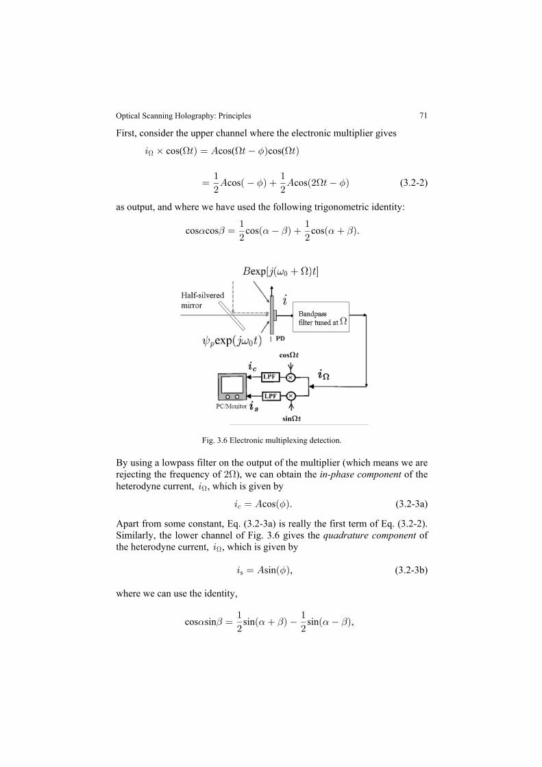
71

First, consider the upper channel where the electronic multiplier gives

3 ‚ >Ñ œ E > Ñ >ÑH cos( cos( cos(H H 9 H

œ E Ð Ñ E Ð# > Ñ" "

# #cos cos (3.2-2)9 H 9

as output, and where we have used the following trigonometric identity:

cos cos cos cos .! " ! " ! "œ Ð Ñ Ð Ñ" "

# #

Fig. 3.6 Electronic multiplexing detection.

By using a lowpass filter on the output of the multiplier (which means we arerejecting the frequency of ), we can obtain the of the#H in-phase component heterodyne current, , which is given by3H

cos . (3.2-3a)3 œ E Ð Ñ- 9

Apart from some constant, Eq. (3.2-3a) is really the first term of Eq. (3.2-2).Similarly, the lower channel of Fig. 3.6 gives the ofquadrature componentthe heterodyne current, , which is given by3H

sin , (3.2-3b)3 œ E Ð Ñs 9

where we can use the identity,

cos sin sin sin , ! " ! " ! "œ Ð Ñ Ð Ñ" "

# #


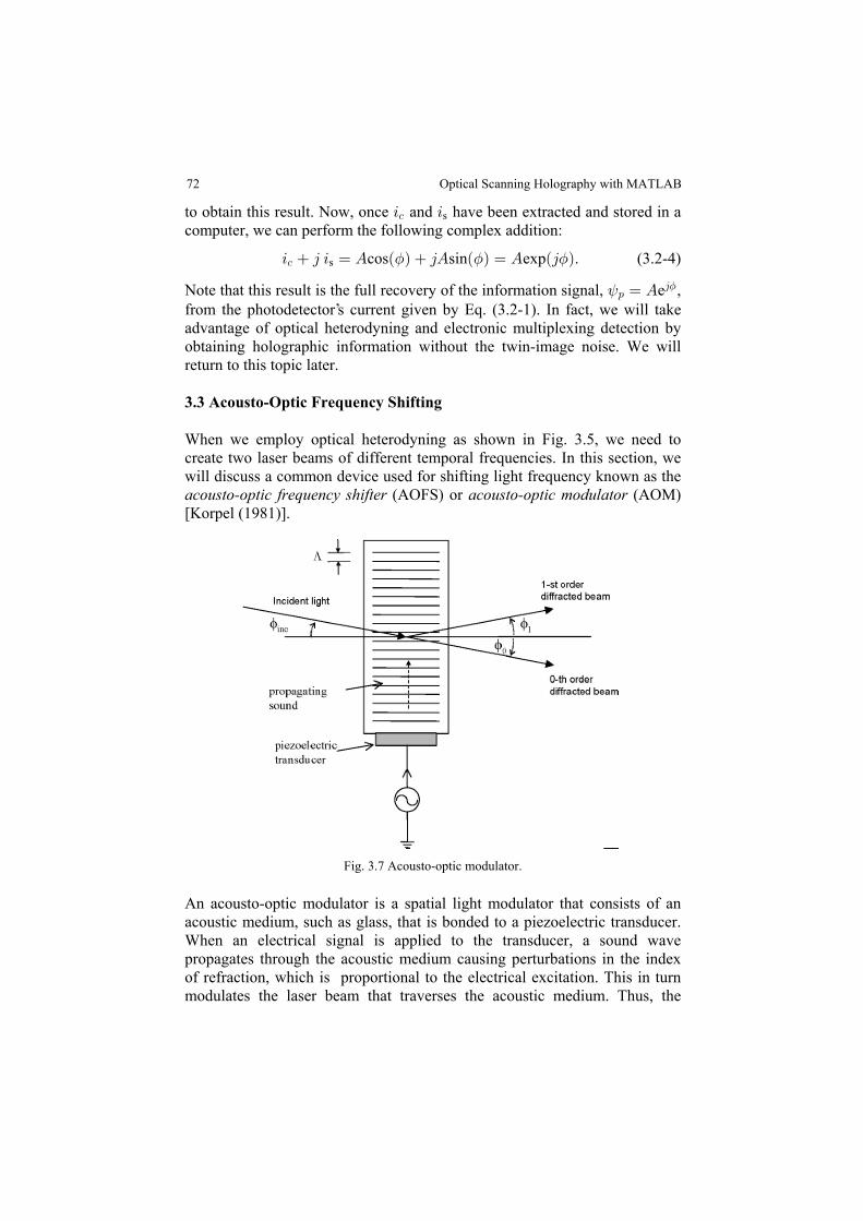
72

to obtain this result. Now, once and have been extracted and stored in a3 3- scomputer, we can perform the following complex addition:

3 4 3 œ E Ð Ñ 4E Ð Ñ œ E Ð4 Ñ- cos sin exp . (3.2-4)s 9 9 9

Note that this result is the full recovery of the information signal, e ,<:4œ E 9

from the photodetector s current given by Eq. (3.2-1). In fact, we will takeadvantage of optical heterodyning and electronic multiplexing detection byobtaining holographic information without the twin-image noise. We willreturn to this topic later.

3.3 Acousto-Optic Frequency Shifting

When we employ optical heterodyning as shown in Fig. 3.5, we need tocreate two laser beams of different temporal frequencies. In this section, wewill discuss a common device used for shifting light frequency known as theacousto-optic frequency shifter acousto-optic modulator (AOFS) or (AOM)[Korpel (1981)].

Fig. 3.7 Acousto-optic modulator.

An acousto-optic modulator is a spatial light modulator that consists of anacoustic medium, such as glass, that is bonded to a piezoelectric transducer.When an electrical signal is applied to the transducer, a sound wavepropagates through the acoustic medium causing perturbations in the indexof refraction, which is proportional to the electrical excitation. This in turnmodulates the laser beam that traverses the acoustic medium. Thus, the

’


73

acousto-optic modulator, as shown in Figure 3.7, may be thought to actsimilar to with an effective grating line separation equal to thephase gratingwavelength, , of the sound in the acoustic medium. As it turns out, for aAvery specific incident angle, , the sound grating splits incident light into9inctwo diffracted beams, namely the 1-st order diffracted beam and the 0-th

" !

One of the simplest explanations used to describe the interactionbetween sound and a laser is to treat the interaction as a collision of particles,namely and . In order fphotons phonons or these particles to have well-defined momenta and energies, we must assume that we have an interactionof plane waves of light and sound. In other words, we assume that the widthof the transducer is sufficiently wide enough to produce plane wave fronts ata single frequency. We will now consider two conservation laws that exist during thecollison: the and the . Theconservation of energy conservation of momentumcondition for conservation of momentum is

, (3.3-1)h5 œ h5 hOt t t !1

where and are the momenta of the incident photon and phonon,h5 hOt t!

respectively, and is the momentum of the scattered photon. , ,h5 5 5t t t !1 1

and are the corresponding wavevectors of the particles, and /2O h œ 2t 1where is . Now, from the conservation of energy, we have2 Planck s constant

h œ h h= = H1 0 , (3.3-2)

where , , and are the energies of the scattered photon, incidenth h h= = H1 0photon, and phonon, respectively. , , and are the corresponding= = H1 0radian frequencies of the particles. After dividing Eq. (3.3-1) by , we haveh

5 œ 5 Ot t t !1 . (3.3-3)

Also, from Eq. (3.3-2), the corresponding conservation of energy takes theform

= = H1 0œ . (3.3-4)

Figure 3.8a) shows the wave-vector interaction diagram and is constructedbased on Eq. (3.3-3). For all practical cases, | | | |, the magnitude ofO ¥ 5t t

!

5 5t t !1 is essentially equal to that of , and the wave-vector triangle shown in

Fig. 3.8a) is, therefore, nearly isosceles. Note that the closed triangle inFigure 3.8a) stipulates that there are certain critical angles of incidence forthe interaction of plane waves of light and sound. The stipulated incidentangle, , is called the , which is given by9inc Bragg angle

9order diffracted beam at angles Fig. 3.7. We shall identify these angles next.

and 9 , respectively. This is shown in

’


74

sin = = , (3.3-5)2 2

Ð ÑO

59

-

AB

0

!

where is the wavenumber of light inside the acoustic5 œ l 5 l œ # Ît0 ! !1 -

medium and is the wavelength of light. is the- 1 A! O œ lOl œ # Ît

wavenumber of sound and is the wavelength of sound. Note that theAdiffracted beams differ in direction by an angle equal to 2 as shown in Fig.9B3.8a). and in Fig. 3.7 must then be equal to .9 9 91 0 B Figure 3.8b) shows that the 1-st diffracted beam is being up-shifted

diffracted beam, , has been upshifted by the amount of the sound=1frequency, . It is also clear that since we really do have a traveling soundHwave, the frequency of the diffracted light is Doppler shifted.

Fig. 3.8 Acousto-optic interaction:a) wave-vector diagram, b) experimental configuration.

The frequencies of sound waves produced in laboratories range fromabout 100 KHz to 3 GHz. Figure 3.9 shows a commercially availableacousto-optic modulator, Model AOM-40, from tIntraAction Corporation. Iuses dense flint glass as an acoustic medium (refractive index 8 μ "Þ'&Ñ!

and operates at a sound center frequency of 40 MHz. Therefore, in Fig.0 œ=

3.9, the sound wave travels in the glass from the left to the right at a velocityof ~ 4000m/s with a sound wavelength of = / ~ 0.l mm. If a He-NeZ Z 0= = =Alaser is used (its wavelength is about 0.6328 in air), its wavelength inside.7the glass is ~ 0.6328 0.3743 . Hence, according to Eq. (3.3-- . .! !7Î8 μ 75), the Bragg angle, inside the acoustic medium is ~ 1.9 10 radian or‚ $

about 0.1 degrees. n Fig. 3.9, we have identified the two diffracted laserIspots at the far background. The incident laser beam (not visible to the eye asit traverses across a transparent medium of glass) is traveling through theglass along the long dimension of the piezoelectric transducer.

Eq. (3.3-4) is called an upshifted interaction because the frequency of thein frequency as is required by Eq. (3.3-4). The interaction described by


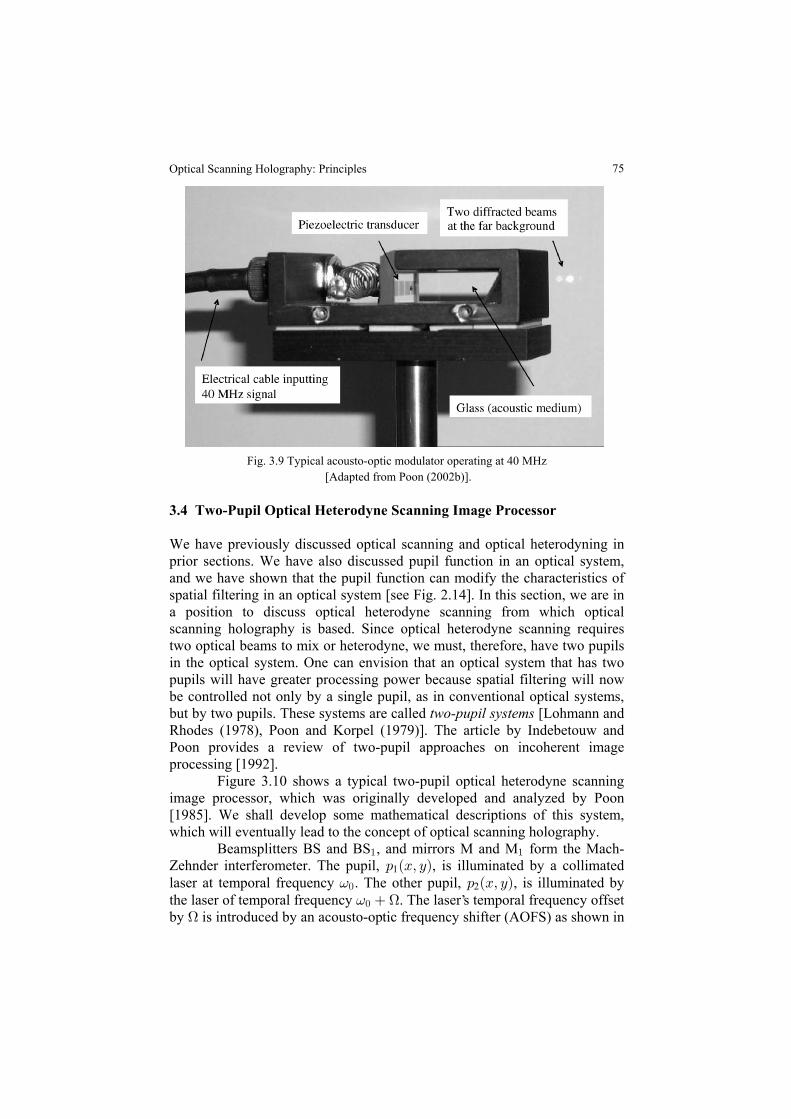
75

Fig. 3.9 Typical acousto-optic modulator operating at 40 MHz [Adapted from Poon (2002b)].

3.4 Two-Pupil Optical Heterodyne Scanning Image Processor

We have previously discussed optical scanning and optical heterodyning inprior sections. We have also discussed pupil function in an optical system,and we have shown that the pupil function can modify the characteristics ofspatial filtering in an optical system [see Fig. 2.14]. In this section, we are ina position to discuss optical heterodyne scanning from which opticalscanning holography is based. Since optical heterodyne scanning requirestwo optical beams to mix or heterodyne, we must, therefore, have two pupilsin the optical system. One can envision that an optical system that has twopupils will have greater processing power because spatial filtering will nowbe controlled not only by a single pupil, as in conventional optical systems,but by two pupils. These systems are called [Lohmann andtwo-pupil systemsRhodes (1978), Poon and Korpel (1979)]. The article by Indebetouw andPoon provides a review of two-pupil approaches on incoherent imageprocessing [1992]. Figure 3.10 shows a typical two-pupil optical heterodyne scanningimage processor, which was originally developed and analyzed by Poon[1985]. We shall develop some mathematical descriptions of this system,which will eventually lead to the concept of optical scanning holography. Beamsplitters BS and BS , and mirrors M and M form the Mach-" "

Zehnder interferometer. The pupil, , is illuminated by a collimated: ÐBß CÑ1laser at temporal frequency . The other pupil, , is illuminated by=! : ÐBß CÑ2the laser of temporal frequency . The laser s temporal frequency offset= H! by is introduced by an acousto-optic frequency shifter (AOFS) as shown inH

’


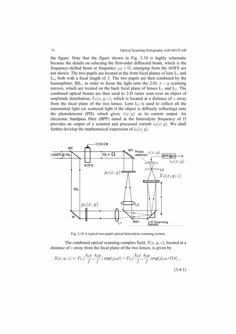
the figure. Note that the figure shown in Fig. 3.10 is highly schematicbecause the details on selecting the first-order diffracted beam, which is thefrequency-shifted beam at frequency , emerging from the AOFS are= H! not shown. The two pupils are located at the front focal planes of lens L and"

L , both with a focal length of . The two pupils are then combined by the# 0beamsplitter, BS , in order to focus the light onto the 2-D, scanning" B Cmirrors, which are located on the back focal plane of lenses L and L The" #Þcombined optical beams are then used to 2-D raster scan over an object ofamplitude distribution, , which is located at a distance of away>!ÐBß Cà DÑ Dfrom the focal plane of the two lenses. Lens L is used to collect all the3transmitted light (or scattered light if the object is diffusely reflecting) ontothe photodetector (PD), which gives as its current output. An3ÐBß CÑelectronic bandpass filter (BPF) tuned at the heterodyne frequency of Hprovides an output of a scanned and processed current . We shall3 ÐBß CÑH

further develop the mathematical expression of .3 ÐBß CÑH

Fig. 3.10 A typical two-pupil optical heterodyne scanning system.

The combined optical scanning complex field, , located at aWÐBß Cà DÑdistance of away from the focal plane of the two lenses, is given byD

WÐBß Cà DÑ œ T Ð Ñ Ð4 >Ñ T Ð Ñ Ò4Ð Ñ>Ó5 B 5 C 5 B 5 C

0 0 0 0"D ! #D !

! ! ! !, exp + , exp + ,= = H

(3.4-1)

76 Optical Scanning Holography with MATLAB

77

where , is the field distribution away from the scanning mirrorsT Ð Ñ D3D5 B 5 C

0 0! !

and through Fresnel diffraction is given by ß

T Ð Ñ œ T Ð Ñ‡ 2ÐBß Cà DÑ 3 œ "ß #5 B 5 C 5 B 5 C

0 0 0 03D 3

! ! ! !, , , . (3.4-2)

In Eq. (3.4-2), , is the field distribution in the back focal plane ofT Ð Ñ35 B 5 C

0 0! !

lenses L and L , and apart from some inessential constant and a constant" #

phase factor, is given by [see Eq. (2.4-6)]

, = ( . (3.4-3)T Ð Ñ Ö: Bß CÑ×5 B 5 C

0 03 3

! !Y º

5Cœ5 CÎ0!

5 œ5 BÎ0B !

Now, as previously mentioned, the combined optical field or the scanningpattern, given by Eq. (3.4-1), is used to two-dimensionally scan an objectwith an amplitude transparency of ; located at a distance from the>0ÐBß C DÑ Dscanning mirrors. According to the principle established by Eq. (3.1-3) foroptical scanning, the photodetector, which responds to the incident intensityof the optical transmitted field or scattered field, generates a current given by

3ÐBß Cà DÑ º l B .C(H

w wWÐB ß C à DÑ ÐB Bß C Cà DÑ .w w w w #!> |

œ T Ð Ñ Ð4 >Ñ T Ð Ñ Ò4Ð Ñ>Ó5 B 5 C 5 B 5 C

0 0 0 0( ºH

’ “"D ! #D !! ! ! !

w w w w

, exp + , exp + = = H

‚ ÐB B ß C C à DÑ .B .C>!w w w w

#º . (3.4-4)

After a bandpass filter (BPF) is tuned to a frequency of , the heterodyneHcurrent from Eq. (3.4-4) becomes

3 ÐBß Cà DÑ œ T Ð Ñ T Ð Ñ5 B 5 C 5 B 5 C

0 0 0 0H Re , ,’(

H"D

! ! ! !w w w w

#D*

‚ l ÐB B ß C C DÑl .B .C Ð4 >Ñ> H!w w # w w; exp , (3.4-5)“

where we have adopted the convention for the phasor as < <: ÐBß Cß >Ñ œRe exp ) , where Re denotes the real part of the contentÒ ÐBß Cß >Ñ Ð4 > Ó ÒÞÓ< H: inside the bracket. Equation (3.4-5) can be written as


3 ÐBß Cà DÑ Ò3 ÐBß Cà DÑ Ð4 >ÑÓH H = Re exp , (3.4-6a):

H

where

3 ÐBß Cà DÑ œ T Ð ÑT Ð Ñ5 B 5 C 5 B 5 C

0 0 0 0H: ( (

H"D

! ! ! !w w w w

#D* , , (3.4-6b)

‚ l ÐB B ß C C DÑl .B .C>!w w # w w;

is the output phasor containing the amplitude and the phase information ofthe heterodyne current. The amplitude and the phase information of thecurrent constitute the scanned and the processed version of the objectl l>!

#and from Eq. (3.4-6), we can write

3 ÐBß Cà DÑ œ 3 ÐBß Cà DÑ ÒÐ > ÐBß Cà DÑÓH H| |cos ,: H 9:

where | |exp . Note that we can re-write Eq. (3.4-6b) in terms of3 œ 3 Ð4 ÑH H: : 9:

the following correlation:

, , ; . (3.4-7)3 ÐBß Cà DÑ œ T Ð Ñ T Ð Ñ l ÐBß C DÑl5 B 5 C 5 B 5 C

0 0 0 0H: "D !

! ! ! !#D

#* Œ >

Similar to conventional optical scanning systems (or incoherent opticalsystems), only the intensity distribution, i.e., will be processed and thel l>!

#

optical system is therefore incoherent. However, is not strictlyl l>!#

processed by an intensity quantity, and as indicated by Eq. (3.4-7) theprocessing element, , can be bipolar or even complex, thereby leadingT T"D #D

*

to the concept of .complex incoherent image processing Equation (3.4-7) relates the input quantity to the output quantity andfrom this we can now define the optical transfer function (OTF) of thesystem to be

; . (3.4-8)SXJ Ð5 ß 5 à DÑ œ Ö3 ÐBß Cà DÑ×Î Öl ÐBß C DÑl ×H HB C !#Y Y >:

By taking the Fourier transform of Eq. (3.4-7) and combining its result withEq. (3.4-8), we obtain the equivalent,

SXJ Ð5 ß 5 à DÑ œ ÖT Ð Ñ T Ð Ñ× Ð Ñ5 B 5 C 5 B 5 C

0 0 0 0H B C

‡ ‡"D #D

! ! ! !Y , , . 3.4-9

In terms of the pupils and , we substitute Eqs. (3.4-2) and (3.4-3) into: :" # Eq. (3.4-9) to get


79

SXJ Ð5 ß 5 à DÑ œ Ò4 Ð5 5 ÑÓD

#5H B C

!

# #B Cexp +

‚ : ÐB C Ñ: ÐB 5 C 5 Ñ Ò4 ÐB 5 C 5 ÑÓ.B .C0 0 D

5 5 0( ( ‡ w w w w w w w w

" #! !

B C B C, , exp .

(3.4-10)This equation was first derived by Poon [1985], and it states that the opticaltransfer function of the system, , can be modified based on theSXJH

we obtainßH

3 ÐBß Cà DÑ œ Ò3 ÐBß Cà DÑ Ð4 >ÑÓH HRe exp: H

œ Ò Ö Öl ÐBß Cà DÑl ×SXJ Ð5 ß 5 à DÑ× Ð4 >ÑÓÞRe expY Y > H" #! B CH

(3.4-11)By defining the spatial impulse response (or the point spread function) of theoptical heterodyne scanning system as

, (3.4-12)2 ÐBß Cà DÑ œ ÖSXJ ×H HY"

we can now re-write Eq. (3.4-11) in the spatial domain as

Re exp . 3.4-133 ÐBß Cà DÑ œ Òl ÐBß Cà DÑl ‡2 ÐBß Cà DÑÓ Ð4 >Ñ Ð ÑH Hš ›> H!#

Equation 3.4-11 or (3.4-13) represents the scanned and processed outputÐ Ñcurrent, which is modulated by a temporal carrier at a frequency of . ByH

H

Re (frequency domain)3 ÐBß Cà DÑ œ Ò Ö Öl l ×SXJ ×Ó- !" #Y Y > H

Ð Ñ3.4-14a#H

and

Im (frequency domain)3 ÐBß Cà DÑ œ Ò Ö Öl l ×SXJ ×Ó= !" #Y Y > H

Im , (spatial domain) 3.4-14bœ Òl l ‡2 ÐBß Cà DÑÓ Ð Ñ>!#

H

where Im[.] denotes the imaginary part of the quantity within the bracket.The subscripts c and s represent the use of cos and sinÐ >Ñ Ð >ÑH Hrespectively, to extract the information from .3H

Eq. (3.4-6a) in terms of SXJselection of the two pupils. Now, by using Eq. (3.4-8) and by re-writing

3 H>mixing with cos( ) or sin( ), we can demodulate and extract the H>

dulation system is shown in Fig. 3.6, and the two outputs are given by

“ ” “ ”


in-phase component or the quadrature component, respectively. The demo-

œ ReÒl> l ‡2 ÐBß Cà DÑÓ (spatial domain)!

In Eqs. (3.4-14), we have assumed that the input object,l ÐBß Cà DÑl D>!

#, is an infinitely thin 2-D object located at a distance of awayfrom the 2-D scanning mirrors shown in Fig. 3.10. To generalize Eqs. (3.4-14) for 3-D objects we need to integrate the equations over the depth, i.e.,ßover , of the 3-D objects. Eqs. (3.4-14) then become [Poon and Kim (1999)]D

3 ÐBß CÑ œ Ò Ö Öl ÐBß Cà DÑl ×SXJ ×.DÓ- !" #Re (3.4-15a)( Y Y > H

œ Ò l ÐBß Cà DÑl ‡2 ÐBß Cà DÑ.DÓRe (3.4-15b)( >!#

H

and

3 ÐBß CÑ œ Ò Ö Öl ÐBß Cà DÑl ×SXJ ×.DÓ= !" #Im (3.4-15c)( Y Y > H

œ Ò l ÐBß Cà DÑl ‡2 ÐBß Cà DÑ.DÓ Ð ÑIm . 3.4-15d( >!#

H

Note that we have left the -dependence out on the left-hand side of Eqs.D(3.4-15) to emphasize that the recorded information is strictly 2-D even for 3-D objects. and represent the scanned and processed current3 ÐBß CÑ 3 ÐBß CÑ- =

(or information) of and can be stored as 2-D records if these currents arel l>!#

stored in synchronization with the signals used to drive the scanningB Cmirrors. Equations (3.4-15) represent the major results of the two-pupiloptical heterodyne scanning of a 3-D object. Figure 3.11 shows the overalltwo-pupil optical heterodyne image processor. The 3-D object isl ÐBß Cà DÑl 3 ÐBß CÑ>! -

#, and the final outputs given by Eqs. (3.4-15) are and3 ÐBß CÑ= . Note that while the input object is given by the amplitudedistribution, , the information that can be processed is the intensity>!ÐBß Cà DÑdistribution given by . As it turns out, this is the incoherentl ÐBß Cà DÑl>!

#

mode of operation for the processor, which has so far been inclusively used

chapter 4, we will further elaborate on some of these applications. In chapter5, when we consider the advancements towards optical scanning holography,we will describe a coherent mode where the complex distribution of theobject can be processed [Indebetouw, Klysubun, Kim, and Poon (2000)].This can be important when we deal with the phase specimens in biologicalapplications.

80

3-D pattern recognition, optical remote sensing, and 3-D cryptography. Infor various applications such as 3-D fluorescence holographic microscopy,


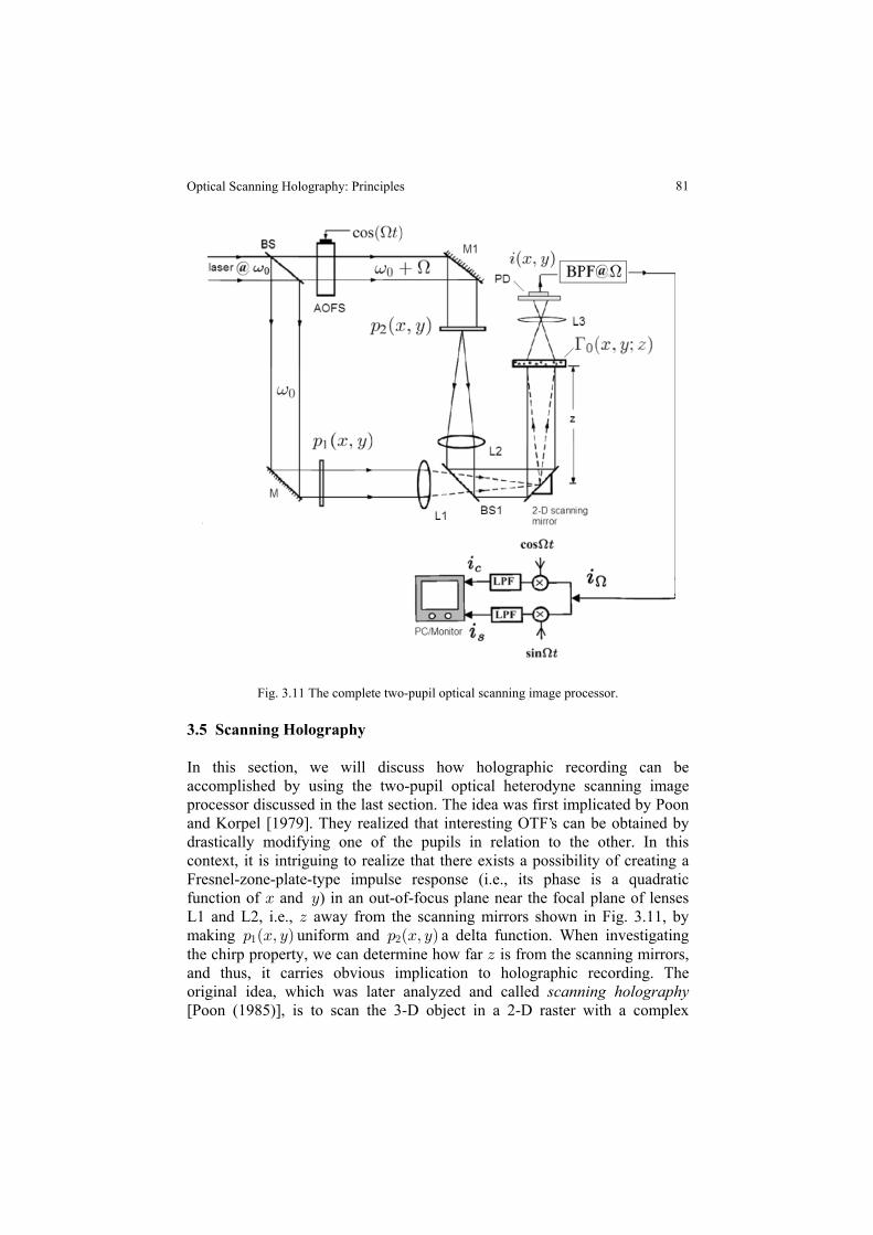
81

Fig. 3.11 The complete two-pupil optical scanning image processor.

3.5 Scanning Holography

In this section, we will discuss how holographic recording can beaccomplished by using the two-pupil optical heterodyne scanning imageprocessor discussed in the last section. The idea was first implicated by Poonand Korpel [1979]. They realized that interesting OTF s can be obtained bydrastically modifying one of the pupils in relation to the other. In thiscontext, it is intriguing to realize that there exists a possibility of creating aFresnel-zone-plate-type impulse response (i.e., its phase is a quadraticfunction of and ) in an out-of-focus plane near the focal plane of lensesB CL1 and L2, i.e., away from the scanning mirrors shown in Fig. 3.11, byDmaking uniform and a delta function. When investigating: ÐBß CÑ : ÐBß CÑ" #

the chirp property, we can determine how far is from the scanning mirrors,Dand thus, it carries obvious implication to holographic recording. Theoriginal idea, which was later analyzed and called scanning holography[Poon (1985)], is to scan the 3-D object in a 2-D raster with a complex

’


Fresnel-zone-plate-type impulse response created by the interference of apoint source and a plane wave emerging from each pupil. A temporalfrequency offset is introduced between the two pupils, and the desired signalfrom a spatially integrating detector is obtained using a heterodyne detection. Hence, for scanning holography we mathematically let : ÐBß CÑ œ ""

and , which are both clearly pictured in Fig. 3.11. With this: ÐBß CÑ œ ÐBß CÑ# $choice of pupils, according to Eq. (3.4-10), the OTF of the heterodynescanning system becomes

SXJ Ð5 ß 5 à DÑ œ Ò 4 Ð5 5 ÑÓD

#5H B C

!

# #B Cº

oshexp +

œ SXJ Ð5 ß 5 à DÑ Ð Ñosh B C , 3.5-1a

and according to Eq. (3.4-12), the corresponding spatial impulse response is

2 ÐBß Cà DÑ œH ºosh

45 45 ÐB C Ñ

# D #DÒ Ó

! !# #

1exp . (3.5-1b)

Apart from the constant phase factor, it is interesting to point out that bycomparing the spatial frequency transfer function in Fourier optics [see Eq.(2.3-13)] to Eq. (3.5-1a), we have

* , (3.5-2a)SXJ Ð5 ß 5 à DÑ œ L Ð5 ß 5 à DÑosh B C B C

and similarly in reference to Eq. (2.3-11), we have

* . (3.5-2b)2 ÐBß Cà DÑ 2 ÐBß Cà DÑH ºosh

œ

From the result of Eq. (3.5-1b) for scanning holography, apart from someconstant, the spatial domain equations, Eqs. (3.4-15b) and (3.4-15d), become

sin3 ÐBß CÑ œ l ÐBß Cà DÑl ‡ Ò Ð .D- !#( š ›>

5 5

# D #DB C ÑÓ

! ! # #

1

(3.5-3a)œ L ÐBß CÑsin

and

(3.5-3b)3 ÐBß CÑ œ l ÐBß Cà DÑl ‡ Ò Ð .D= !#( š ›>

5 5

# D #DB C ÑÓ

! ! # #

1cos

,œ L ÐBß CÑcos


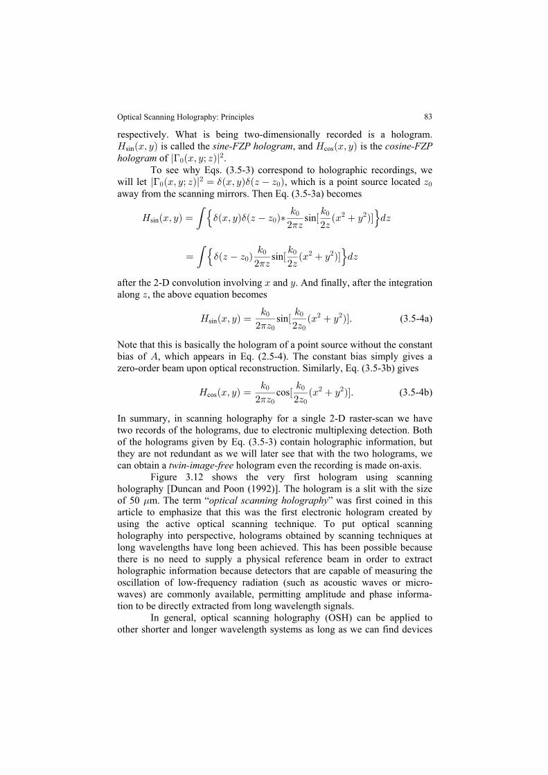
83

respectively. What is being two-dimensionally recorded is a hologram.L ÐBß CÑ L ÐBß CÑsin cos is called the , and is the sine-FZP hologram cosine-FZPhologram of .l ÐBß Cà DÑl>!

#

To see why Eqs. (3.5-3) correspond to holographic recordings, wewill let , which is a point source located l ÐBß Cà DÑl œ ÐBß CÑ ÐD D Ñ D> $ $! ! !

#

away from the scanning mirrors. Then Eq. (3.5-3a) becomes

sinL ÐBß CÑ œ ÐBß CÑ ÐD D Ñ‡ Ò Ð .Dsin ( š ›$ $ !5 5

# D #DB C ÑÓ

! ! # #

1

sinœ ÐD D Ñ Ò Ð .D( š ›$ !5 5

# D #DB C ÑÓ

! ! # #

1

after the 2-D convolution involving and . And finally, after the integrationB Calong , the above equation becomesD

L ÐBß CÑ œ Ò ÐD D

sin5 5

# #B C ÑÓ

! ! # #

1 ! !sin . (3.5-4a)

Note that this is basically the hologram of a point source without the constantbias of , which appears in Eq. (2.5-4). The constant bias simply gives aEzero-order beam upon optical reconstruction. Similarly, Eq. (3.5-3b) gives

L ÐBß CÑ œ Ò ÐD D

cos5 5

# #B C ÑÓ

! ! # #

1 ! !cos . (3.5-4b)

In summary, in scanning holography for a single 2-D raster-scan we havetwo records of the holograms, due to electronic multiplexing detection. Bothof the holograms given by Eq. (3.5-3) contain holographic information, butthey are not redundant as we will later see that with the two holograms, wecan obtain a hologram even the recording is made on-axis. twin-image-free Figure 3.12 shows the very first hologram using scanningholography [Duncan and Poon (1992)]. The hologram is a slit with the sizeof 50 m. The term was first coined in this. optical scanning holographyarticle to emphasize that this was the first electronic hologram created byusing the active optical scanning technique. To put optical scanningholography into perspective, holograms obtained by scanning techniques atlong wavelengths have long been achieved. This has been possible becausethere is no need to supply a physical reference beam in order to extractholographic information because detectors that are capable of measuring the

In general, optical scanning holography (OSH) can be applied toother shorter and longer wavelength systems as long as we can find devices

“ ”

oscillation of low-frequency radiation (such as acoustic waves or micro-waves) are commonly available, permitting amplitude and phase informa-tion to be directly extracted from long wavelength signals.


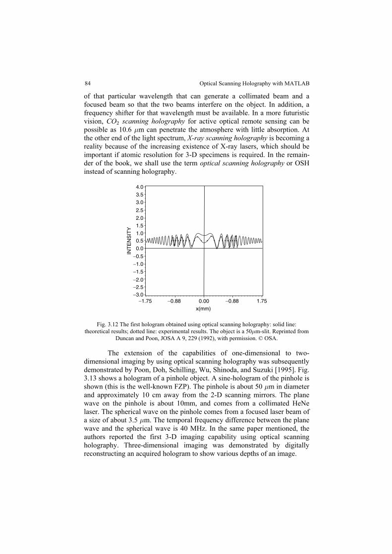
of that particular wavelength that can generate a collimated beam and afocused beam so that the two beams interfere on the object. In addition, afrequency shifter for that wavelength must be available. In a more futuristicvision, for active optical remote sensing can beCO scanning holography#

possible as 10.6 m can penetrate the atmosphere with little absorption. At.the other end of the light spectrum, is becoming aX-ray scanning holographyreality because of the increasing existence of X-ray lasers, which should be

Fig. 3.12 The first hologram obtained using optical scanning holography: solid line:theoretical results; dotted line: experimental results. The object is a 50 m-slit. Reprinted from.

Duncan and Poon, JOSA A 9, 229 (1992), with permission. © OSA.

The extension of the capabilities of one-dimensional to two-dimensional imaging by using optical scanning holography was subsequentlydemonstrated by Poon, Doh, Schilling, Wu, Shinoda, and Suzuki [1995]. Fig.3.13 shows a hologram of a pinhole object. A sine-hologram of the pinhole isshown (this is the well-known FZP). The pinhole is about 50 m in diameter.and approximately 10 cm away from the 2-D scanning mirrors. The planewave on the pinhole is about 10mm, and comes from a collimated HeNelaser. The spherical wave on the pinhole comes from a focused laser beam ofa size of about 3.5 m. The temporal frequency difference between the plane.wave and the spherical wave is 40 MHz. In the same paper mentioned, theauthors reported the first 3-D imaging capability using optical scanningholography. Three-dimensional imaging was demonstrated by digitallyreconstructing an acquired hologram to show various depths of an image.

84

important if atomic resolution for 3-D specimens is required. In the remain-der of the book, we shall use the term optical scanning holography or OSH

−3.0−1.75 −0.88 0.00 −0.88 1.75

−2.5−2.0

−1.5

−1.0

−0.5

0.0

0.51.0

1.52.0

2.5

3.0

3.5

4.0

INT

EN

SIT

Y

x(mm)


instead of scanning holography.

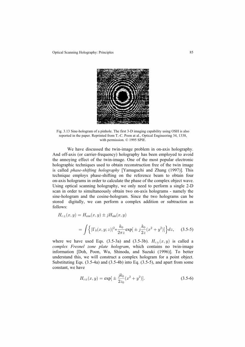
85

Fig. 3.13 Sine-hologram of a pinhole. The first 3-D imaging capability using OSH is alsoreported in the paper. Reprinted from T.-C. Poon at al., Optical Engineering 34, 1338,

with permission. © 1995 SPIE.

We have discussed the twin-image problem in on-axis holography.And off-axis (or carrier-frequency) holography has been employed to avoidthe annoying effect of the twin-image. One of the most popular electronicholographic techniques used to obtain reconstruction free of the twin imageis called [Yamaguchi and Zhang (1997)] Thisphase-shifting holography .

Using optical scanning holography, we only need to perform a single 2-Dscan in order to simultaneously obtain two on-axis holograms - namely thesine-hologram and the cosine-hologram. Since the two holograms can bestored digitally, we can perform a complex addition or subtraction asfollows:

L ÐBß CÑ œ-„ L ÐBß CÑ „ 4L ÐBß CÑcos sin

, (3.5-5)œ l ÐBß Cà DÑl ‡ Ò „ 4 Ð .D( š ›>!# 5 5

# D #DB C ÑÓ

! ! # #

1exp

where we have used Eqs. (3.5-3a) and (3.5-3b). L ÐBß CÑ-„ is called acomplex Fresnel zone plate hologram, which contains no twin-imageinformation [Doh, Poon, Wu, Shinoda, and Suzuki (1996)]. To betterunderstand this, we will construct a complex hologram for a point object.Substituting Eqs. (3.5-4a) and (3.5-4b) into Eq. (3.5-5), and apart from someconstant, we have

. (3.5-6)L ÐBß CÑ œ Ò „ Ð4

D-„

!exp

5

#B C ÑÓ

! # #

on-axis holograms in order to calculate the phase of the complex object wave.technique employs phase-shifting on the reference beam to obtain four


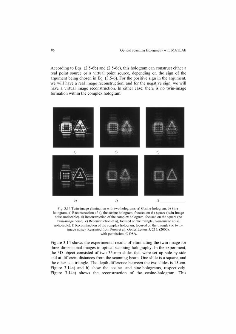
According to Eqs. (2.5-6b) and (2.5-6c), this hologram can construct either areal point source or a virtual point source, depending on the sign of theargument being chosen in Eq. (3.5-6). For the positive sign in the argument,we will have a real image reconstruction, and for the negative sign, we willhave a virtual image reconstruction. In either case, there is no twin-imageformation within the complex hologram.

Fig. 3.14 Twin-image elimination with two holograms: a) Cosine-hologram. b) Sine-hologram. c) Reconstruction of a), the cosine-hologram, focused on the square (twin-imagenoise noticeable). d) Reconstruction of the complex hologram, focused on the square (no

twin-image noise). e) Reconstruction of a), focused on the triangle (twin-image noisenoticeable). f) Reconstruction of the complex hologram, focused on the triangle (no twin-

image noise). Reprinted from Poon et al., Optics Letters 5, 215, (2000), with permission. © OSA.

Figure 3.14 shows the experimental results of eliminating the twin image forthree-dimensional images in optical scanning holography. In the experiment,the 3D object consisted of two 35-mm slides that were set up side-by-sideand at different distances from the scanning beam. One slide is a square, andthe other is a triangle. The depth difference between the two slides is 15-cm.Figure 3.14a) and b) show the cosine- and sine-holograms, respectively.Figure 3.14c) shows the reconstruction of the cosine-hologram. This


87

reconstruction is focused on the square object but is spoiled by twin-imagenoise. In Fig. 3.14d), where the complex hologram is used to reconstruct andfocus on the square object, twin-image noise is not present. In Fig. 3.14e),the cosine hologram reconstructs an image that is focused on the triangle butspoiled by twin-image noise. In fig. 3.14f), the complex hologram gives areconstruction without twin-image noise. Thus, the elimination of twin-image in optical scanning holography has been demonstrated using only twoholograms. In the demonstration, the use of digital reconstruction has beenemployed. By using two SLM’s (one for the display of a sine-hologram andthe other for a cosine-hologram), we can achieve all-optical reconstruction.However, this has yet to be demonstrated optically [Poon (2006)].

Example 3.1 MATLAB Example: Optical Scanning Holography

By substituting the OTF of optical scanning holography, given by Eq. (3.5-1a), into Eqs. (3.4-15a) and (3.4-15c), the sine-hologram and the cosine-hologram will be expressed in terms of spatial frequencies. Therefore, wehave

3 ÐBß CÑ œ Ò Ö Öl ÐBß Cà DÑl ×SXJ 5 ß 5 à D ×.DÓ- ! B C" #Re ( )( Y Y > osh

(3.5-7a)œ L ÐBß CÑsin

and

3 ÐBß CÑ œ Ò Ö Öl ÐBß Cà DÑl ×SXJ 5 ß 5 à D ×.DÓs oshIm ( )( Y Y >" #! B C

, (3.5-7b)œ L ÐBß CÑcos

where ( ) exp + . For this example, we areSXJ 5 ß 5 à D œ Ò 4 Ð5 5 ÑÓosh B CD#5

# #B C!

assuming a planar object to be at a distance of away from the x-y scanningD!mirrors, i.e., , where is the planarl ÐBß Cà DÑl œ MÐBß CÑ ÐD D Ñ MÐBß CÑ> $! !

#

intensity distribution shown in Fig. 3.15a). For the planar intensity object,after integrating over , Eqs. (3.5-7a) and (3.5-7b) becomeD

Re ( ) (3.5-8a)L ÐBß CÑ œ Ò Ö ÖMÐBß CÑ×SXJ 5 ß 5 à D ×Ósin oshY Y"B C !

and

Im ( ) , (3.5-8b)L ÐBß CÑ œ Ò Ö ÖMÐBß CÑ×SXJ 5 ß 5 à D ×Ócos oshY Y"B C !


respectively. The above holograms are simulated and shown in Fig. 3.15b)and Fig. 3.15c), respectively where sigma in OSH.m listedœ D Î#5 œ #Þ!! !

in Table 3.1. We can also construct a complex FZP hologram by using Eq.(3.5-5):

L ÐBß CÑ œ-+ L ÐBß CÑ 4L ÐBß CÑcos sin

( ) (3.5-9)œ ÖMÐBß CÑ×SXJ 5 ß 5 à DY Y"B C !Ö ×osh .

For digital reconstruction, we will simply convolve the above hologramswith the spatial impulse response in order to simulate Fresnel diffraction for adistance of . To obtain real image reconstruction formed in front of theD!hologram, we will use the following equation:

L ÐBß CÑ‡2ÐBß Cà D Ñany ! ,

where represents any one of the above holograms, i.e., the sine-L ÐBß CÑanyhologram, the cosine-hologram or the complex hologram. In OSH.m, theabove equation is implemented in the Fourier domain using the followingequation [see Eqs. (1.2-3a) and (1.2-3b)]:

Reconstructed real image

º ÖL ÐBß CÑ×LÐ5 ß 5 à D ÑY Y"B C !Ö ×any

*( ) , (3.5-10)œ ÖL ÐBß CÑ×SXJ 5 ß 5 à DY Y"B C !Ö ×any osh

where we have used Eq. (3.5-2a) to relate with the spatial frequencySXJoshresponse, , to obtain the last step. Figures 3.15d), e) and f ) showLÐ5 ß 5 à D ÑB C !

the reconstruction of the sine-hologram, the cosine-hologram, and thecomplex hologram, respectively. Note that if the complex hologram is constructed as

,L ÐBß CÑ œ- L ÐBß CÑ 4L ÐBß CÑcos sin

then it will have a reconstructed virtual image that is located at a distance ofD! behind the hologram. However, if we perform

L ÐBß CÑ‡2ÐBß Cà D Ñ- !

for reconstruction, we will see a severely out-of-focus image formed at!

diffraction pattern of the original object at a distance of .D œ #D!


D œ D as shown in Fig. (3.15g), which is equivalent to the Fresnel

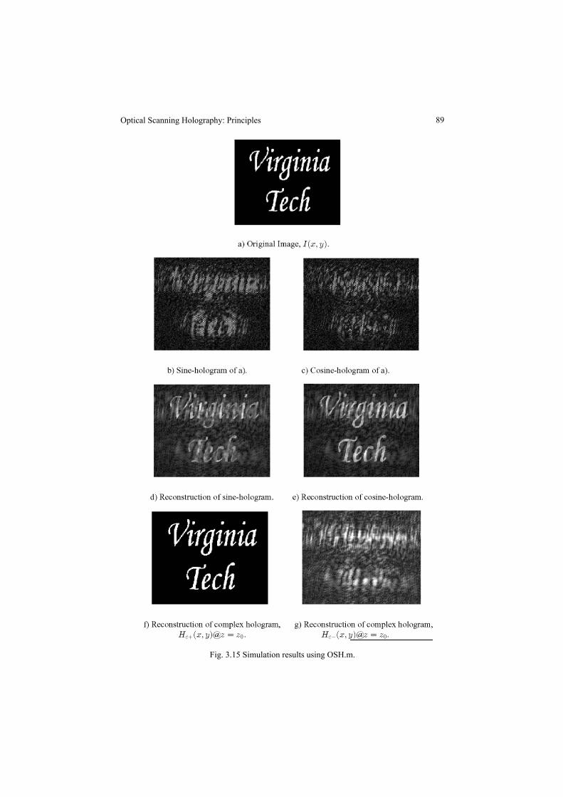
89

Fig. 3.15 Simulation results using OSH.m.


Table 3.1 OSH.m : m-file for illustrating optical scanning holography.------------------------------------------------------% OSH.m% Adapted from "Contemporary Optical Image Processing with MATLAB,"% by Ting-Chung Poon and Partha Banerjee, Table 7.2,% Pages 222-223, Elsevier (2001).

clear all,%%Reading input bitmap fileI=imread('vatech.bmp','bmp');I=I(:,:,1);figure(1)%displaying inputcolormap(gray(255));image(I)title('Original image')axis offpause

%%Creating OTFosh with SIGMA=z/2*k0 (Eq.(3.5-1a))ROWS=256;COLS=256;sigma=2.0; %not necessary to scale%kx,ky are spatial frequenciesky=-12.8;for r=1:COLS, kx=-12.8; for c=1:ROWS, OTFosh(r,c)=exp(-j*sigma*kx*kx-j*sigma*ky*ky); kx=kx+.1; end ky=ky+.1;endmax1=max(OTFosh);max2=max(max1);scale=1.0/max2;OTFosh=OTFosh.*scale;

%Recording hologram% Taking Fourier transform of IFI=fft2(I);FI=fftshift(FI);max1=max(FI);max2=max(max1);scale=1.0/max2;FI=FI.*scale;% FH is the recorded hologram in Fourier domainFH=FI.*OTFosh;H=ifft2(FH);max1=max(H);max2=max(max1);scale=1.0/max2;


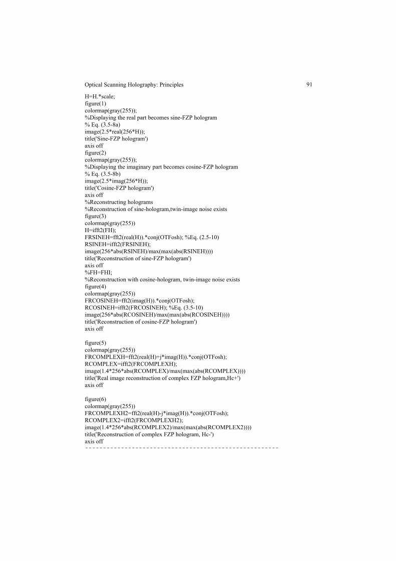
91

H=H.*scale;figure(1)colormap(gray(255));%Displaying the real part becomes sine-FZP hologram% Eq. (3.5-8a)image(2.5*real(256*H));title('Sine-FZP hologram')axis offfigure(2)colormap(gray(255));%Displaying the imaginary part becomes cosine-FZP hologram% Eq. (3.5-8b)image(2.5*imag(256*H));title('Cosine-FZP hologram')axis off%Reconstructing holograms%Reconstruction of sine-hologram,twin-image noise existsfigure(3)colormap(gray(255))H=ifft2(FH);FRSINEH=fft2(real(H)).*conj(OTFosh); %Eq. (2.5-10)RSINEH=ifft2(FRSINEH);image(256*abs(RSINEH)/max(max(abs(RSINEH))))title('Reconstruction of sine-FZP hologram')axis off%FH=FHI;%Reconstruction with cosine-hologram, twin-image noise existsfigure(4)colormap(gray(255))FRCOSINEH=fft2(imag(H)).*conj(OTFosh);RCOSINEH=ifft2(FRCOSINEH); %Eq. (3.5-10)image(256*abs(RCOSINEH)/max(max(abs(RCOSINEH))))title('Reconstruction of cosine-FZP hologram')axis off

figure(5)colormap(gray(255))FRCOMPLEXH=fft2(real(H)+j*imag(H)).*conj(OTFosh);RCOMPLEX=ifft2(FRCOMPLEXH);image(1.4*256*abs(RCOMPLEX)/max(max(abs(RCOMPLEX))))title('Real image reconstruction of complex FZP hologram,Hc+')axis off

figure(6)colormap(gray(255))FRCOMPLEXH2=fft2(real(H)-j*imag(H)).*conj(OTFosh);RCOMPLEX2=ifft2(FRCOMPLEXH2);image(1.4*256*abs(RCOMPLEX2)/max(max(abs(RCOMPLEX2))))title('Reconstruction of complex FZP hologram, Hc-')axis off------------------------------------------------------


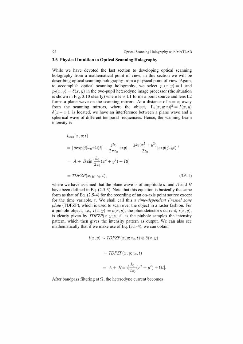
3.6 Physical Intuition to Optical Scanning Holography

While we have devoted the last section to developing optical scanningholography from a mathematical point of view, in this section we will bedescribing optical scanning holography from a physical point of view. Again,to accomplish optical scanning holography, we select and: ÐBß CÑ œ ""

: ÐBß CÑ œ ÐBß CÑ# $ in the two-pupil heterodyne image processor (the situationis shown in Fig. 3.10 clearly) where lens L1 forms a point source and lens L2forms a plane wave on the scanning mirrors. At a distance of awayD œ D!from the scanning mirrors, where the object, l ÐBß Cà DÑl œ MÐBß CÑ>!

#

$ÐD D Ñ! , is located, we have an interference between a plane wave and aspherical wave of different temporal frequencies. Hence, the scanning beamintensity is

M ÐBß Cà >Ñscan

œ l + Ò4Ð Ñ>Ó Ò Ó Ð4 >Ñl45 45 ÐB C Ñ

D #Dexp + exp exp

2= H =

1! !

! !

! !

#2 2

2

œ E F Ò ÐB C Ñ >Ó5

Dsin !

!

2 2 H

, (3.6-1)œ ÐBß Cà D ß >ÑTDFZP !

where we have assumed that the plane wave is of amplitude , and and + E Fhave been defined in Eq. (2.5-3). Note that this equation is basically the sameform as that of Eq. (2.5-4) for the recording of an on-axis point source exceptfor the time variable, . We shall call this a > time-dependent Fresnel zoneplate (TDFZP), which is used to scan over the object in a raster fashion. Fora pinhole object, i.e., , the photodetector s current, ,MÐBß CÑ œ ÐBß CÑ 3ÐBß CÑ$is clearly given by as the pinhole samples the intensityTDFZPÐBß Cà D ß >Ñ!

pattern, which then gives the intensity pattern as output. We can also seemathematically that if we make use of Eq. (3.1-4), we can obtain

3ÐBß CÑ μ ÐBß Cà D ß >ÑTDFZP ! Œ ÐBß CÑ$

œ ÐBß Cà D ß >ÑTDFZP !

œ E F Ò ÐB C Ñ >ÓÞ5

D

2sin !

!

2 2 H

After bandpass filtering at , the heterodyne current becomesH

92

’


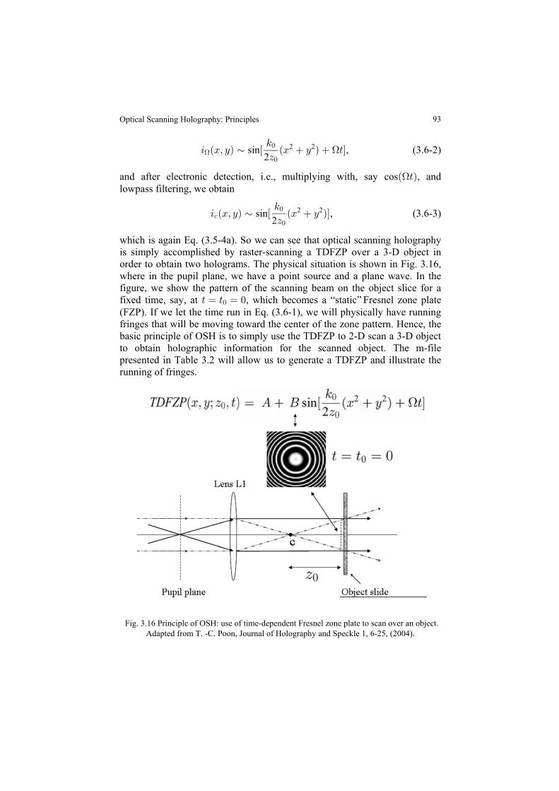
93

, (3.6-2)2

3 ÐBß CÑ μ Ò ÐB C Ñ >Ó5

DH sin !

!

2 2 H

and after electronic detection, i.e., multiplying with, say cos , andÐ >ÑHlowpass filtering, we obtain

3 ÐBß CÑ μ Ò ÐB C ÑÓ5

D-

!

!sin

2, (3.6-3)2 2

which is again Eq. (3.5-4a). So we can see that optical scanning holographyis simply accomplished by raster-scanning a TDFZP over a 3-D object inorder to obtain two holograms. The physical situation is shown in Fig. 3.16,where in the pupil plane, we have a point source and a plane wave. In thefigure, we show the pattern of the scanning beam on the object slice for afixed time, say, at , which becomes a “static” Fresnel zone plate> œ > œ !!

(FZP). If we let the time run in Eq. (3.6-1), we will physically have runningfringes that will be moving toward the center of the zone pattern. Hence, thebasic principle of OSH is to simply use the TDFZP to 2-D scan a 3-D objectto obtain holographic information for the scanned object. The m-filepresented in Table 3.2 will allow us to generate a TDFZP and illustrate therunning of fringes.

Fig. 3.16 Principle of OSH: use of time-dependent Fresnel zone plate to scan over an object.Adapted from T. -C. Poon, Journal of Holography and Speckle 1, 6-25, (2004).


We can also select the pupils differently to achieve optical scanningholography as long as we can create a time-dependent FZP to scan the 3-Dobject. For example, we can select and 1: ÐBß CÑ œ ÐBß CÑ : ÐBß CÑ œ" #$instead of 1 and as we had previously: ÐBß CÑ œ : ÐBß CÑ œ ÐBß CÑ" # $discussed in the two-pupil heterodyne image processor. Then, the scanningintensity become

M ÐBß Cà >Ñscan

œ l + Ð4 >Ñ Ò Ó Ò4Ð Ñ>Ó l45 45 B C Ñ

D #Dexp exp exp +

2(

= = H1

! !! !

! !

#2 2


D

2sin !

!

2 2 H

. (3.6-4)œ ÐBß Cà D ß >ÑTDFZP !

This will give fringes running away from the center of the zone, and this canbe verified by changing the sign in front of B in the expression ofFZP(ii,jj,kk) in the TDFZP.m file. As it turns out, this scanning beam givesthe same expression for the sine-hologram given by Eq. (3.5-3a). However,the expression for the cosine-hologram is different with a negative sign infront of it. Note that the errors and sensitivities produced by the heterodynemethod, as well as the impact created by these errors, will not be discussed inthis book. Readers should refer to Section 5.4 of the Handbook ofHolographic Interferometry [Kreis, 2005], which will provide insight into thepractical limitations of heterodyning holographic interferometry. When H is set to zero, we have and the time-dependenthomodyningFresnel zone plate becomes static. Now by introducing phase shifts betweenthe two interfering waves that are used to generate the Fresnel zone plate,one can obtain three holograms (as a result of three different phase shifts) toalternatively solve the twin-image problem in optical scanning holography[Rosen, Indebetouw and Brooker (2006)].

Table 3.2 TDFZP.m : m-file for illustrating running fringes in TDFZP.------------------------------------------------------% TDFZP.m% Illustration of running fringes in TDFZP% The author thanks Kelly Dobson for her initial programming

clear;B=10.01*10^6; %temporal frequency, arbitraryD=6; %Scale arbitrary

t=linspace(0,1,35);x=linspace(-2.5,2.5,256);y=linspace(-2.5,2.5,256);

94

“ ”


95

for ii=1:length(x) for jj=1:length(y) for kk=1:length(t) FZP(ii,jj,kk)=(1+sin(D*(x(ii)^2+y(jj)^2)+B*t(kk))); %TDFZP end endend

for ll=1:length(t) max1=max(FZP(:,:,ll)); max2=max(max1); scale=1/max2; FZP(:,:,ll)=FZP(:,:,ll).*scale;figure(ll);colormap(gray(256));image(256*FZP(:,:,ll));axis offF(ll)=getframe;end

movie(F,10)------------------------------------------------------

References

3.1 Duncan, B.D. and T.-C. Poon (1992). Gaussian beam analysis of optical scanningholography, 9, 229-236.Journal of the Optical Society of America A

3.2 Doh, K., T.-C. Poon, M. Wu, K. Shinoda, and Y. Suzuki (1996).

141.3.3 General Scanning. http://www.gsig.com/scanners/3.4 Indebetouw, G. and T.-C. Poon (1992). Novel approaches of incoherent image

processing with emphasis on scanning methods, 31, 2159-Optical Engineering 2167.

3.5 Indebetouw, G., P. Klysubun, T. Kim, and T.-C. Poon (2000). Imaging propertiesof scanning holographic microscopy, Journal of the Optical Society of America A17, 380-390.

3.6 Indebetouw, G and W. Zhong (2006). Scanning holographic microscopy of three-dimensional fluorescent specimens, .Journal of the Optical Society of America A23, 1699-1707.

3.7 IntraAction Corp. http://www.intraaction.com/3.8 T.-C. Poon (1999). Extraction of 3-D location of matched 3-D object

using power fringe-adjusted filtering and Wigner analysis, 38,Optical Engineering 2176-2183.

3.9 Korpel, A. (1981). Acousto-optics-a review of fundamentals, Proceedings of theIEEE 69, 48-53.

3.10 Kreis, T. (2005). . Wiley-VCH GmbH &Handbook of Holographic InterferometryCo. KGaA, Weinheim.

3.11 Lohmann, A. W. and W. T. Rhodes (1978). Two-pupil synthesis of optical transferfunctions, 17, 1141-1150. Applied Optics

“”

“”

“”

“”

“”

“”

“ ”

“”

Kim, T and


Twin-imageLaser & Optics Technology 28, 135-elimination in optical scanning holography,

3.12 Poon, T.-C. (1985). Scanning holography and two-dimensional image processingby acousto-optic two-pupil synthesis, Journal of the Optical Society of America A4, 521-527

3.13 Poon, T.-C. (2002a). Three-dimensional television using optical scanningholography,” 3, 12-16.Journal of Information Display

3.14 Poon, T.-C. (2002b). Acousto-Optics, Encyclopedia of Physical Science andTechnology, Academic Press.

3.15 Poon, T.-C. (2004). Recent progress in optical scanning holography , Journal ofHolography and Speckle 1, 6-25.

3.16 Poon, T.-C. (2006). Horizontal-parallax-only optical scanning holography, inchapter 10 of Digital Holography and Three-Dimensional Display: Principles andApplications , T.-C. Poon ed., Springer, New York, USA.

3.17 Poon, T.-C. and A. Korpel. (1979). Optical transfer function of an acousto-opticheterodyning image processor, 4, 317-319.Optics Letters

3.18 Poon, T.-C., K. Doh, B. Schilling, M. Wu, K. Shinoda, and Y. Suzuki (1995).

3.19 Poon, T.-C. and T. Kim (1999). Optical image recognition of three-dimensionalobjects, 38, 370-381.Applied Optics

3.20 Poon, T.-C., T. Kim, G. Indebetouw, B. W. Schilling, M. H. Wu, K. Shinoda, andY. Suzuki (2000). Twin-image elimination experiments for three-dimensionalimages in optical scanning holography, 25, 215-217.Optics Letters

3.21 Poon T.-C. and P. P. Banerjee (2001). Contemporary Optical Image Processingwith MATLAB . ® Elsevier, Oxford, UK.

3.22 Poon, T.-C., T. Kim and K. Doh (2003) Optical scanning cryptography for securewireless transmission, 42, 6496-6503.Applied Optics

3.23 Poon, T.-C. and T. Kim (2006). WorldEngineering Optics with MATLAB®. Scientific Publishing Co., Singapore.

3.24 Pratt, W.K. (1969). , John Wiley & Sons.Laser Communications Systems3.25 Rosen, J., G. Indebetouw, and G. Brooker. Homodyne scanning holography,

Optics Express 14, 4280-4285.3.26 Yamaguchi, I. and T. Zhang (1997). Phase-shifting digital holography, Optics

Letters 22, 1268-1270.

96

“”

“

“ ”

“ ”

“ ”

“”

“ ”

“”

“”

“”

“ ”

“ ”

Optical Engi-Three-dimensional microscopy by optical scanning holography,neering 34, 1338–1344.


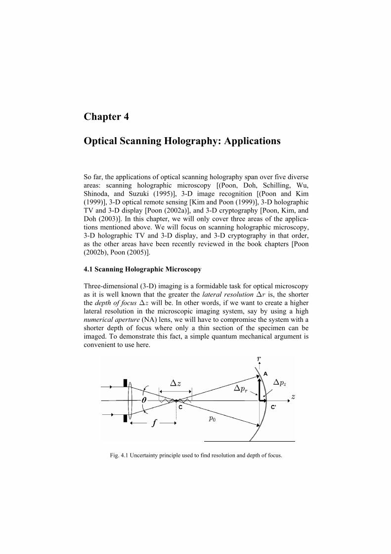
Chapter 4

Optical Scanning Holography: Applications

So far, the applications of optical scanning holography span over five diverseareas: scanning holographic microscopy [(Poon, Doh, Schilling, Wu,Shinoda, and Suzuki (1995)], 3-D image recognition [(Poon and Kim(1999)], 3-D optical remote sensing [Kim and Poon (1999)], 3-D holographicTV and 3-D display [Poon (2002a)], and 3-D cryptography [Poon, Kim, and

4.1 Scanning Holographic Microscopy

Three-dimensional (3-D) imaging is a formidable task for optical microscopyas it is well known that the greater the is, the shorterlateral resolution ?<the will be. In other words, if we want to create a higherdepth of focus ?Dlateral resolution in the microscopic imaging system, say by using a highnumerical aperture (NA) lens, we will have to compromise the system with ashorter depth of focus where only a thin section of the specimen can beimaged. To demonstrate this fact, a simple quantum mechanical argument isconvenient to use here.

Fig. 4.1 Uncertainty principle used to find resolution and depth of focus.

Doh (2003)]. In this chapter, we will only cover three areas of the applica-tions mentioned above. We will focus on scanning holographic microscopy,3-D holographic TV and 3-D display, and 3-D cryptography in that order,as the other areas have been recently reviewed in the book chapters [Poon(2002b), Poon (2005)].

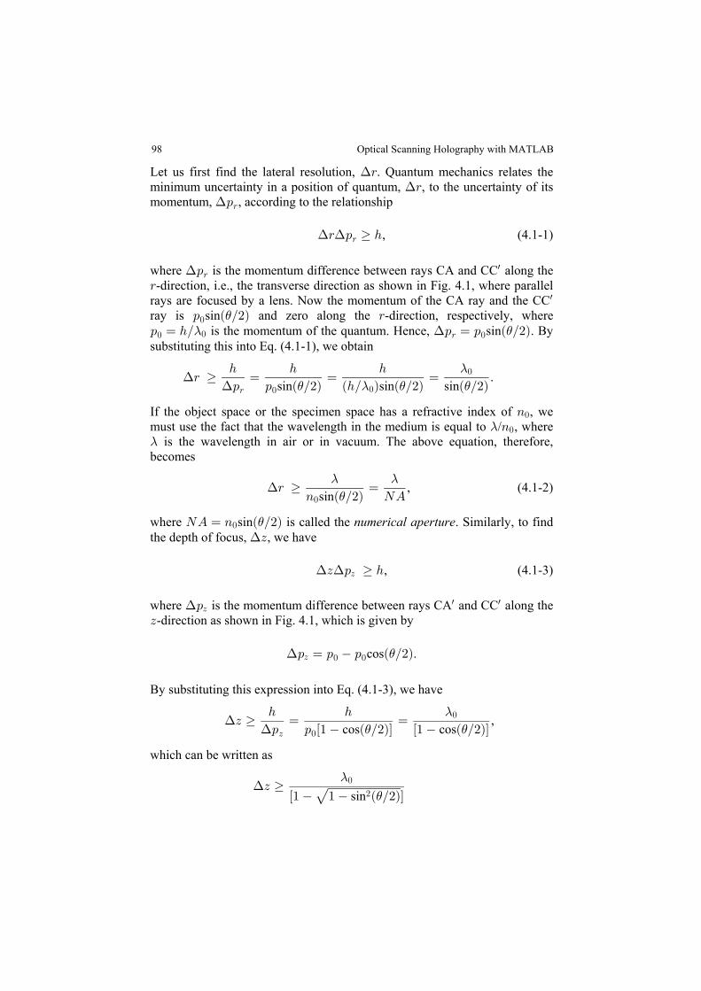
Let us first find the lateral resolution, . Quantum mechanics relates the?<minimum uncertainty in a position of quantum, , to the uncertainty of its?<momentum, , according to the relationship?:<

? ?< : 2< , (4.1-1)

where is the momentum difference between rays CA and CC along the?:<w

<-direction, i.e., the transverse direction as shown in Fig. 4.1, where parallelrays are focused by a lens. Now the momentum of the CA ray and the CCw

ray is sin and zero along the -direction, respectively, where: Ð Î#Ñ <! ): œ 2Î : œ : Ð Î#Ñ! < !!- ? ) is the momentum of the quantum. Hence, sin . Bysubstituting this into Eq. (4.1-1), we obtain

?? ) - ) )

-< œ œ œ

2 2 2

: : Ð Î#Ñ Ð2Î Ñ Ð Î#Ñ Ð Î#Ñ .

sin sin sin< ! !

!

If the object space or the specimen space has a refractive index of , we8!

must use the fact that the wavelength in the medium is equal to / , where- 8!

- is the wavelength in air or in vacuum. The above equation, therefore,becomes

, (4.1-2)sin

?- -

)< œ

8 Ð Î#Ñ RE!

where sin is called the . Similarly, to findRE œ 8 Ð Î#Ñ! ) numerical aperturethe depth of focus, , we have?D

, (4.1-3)? ?D : 2D

where is the momentum difference between rays CA and CC along the?:Dw w

D-direction as shown in Fig. 4.1, which is given by

? ): œ : : Ð Î#ÑD ! !cos .

By substituting this expression into Eq. (4.1-3), we have

?? ) )

-D œ œ

2 2

: : Ò" Ð Î#ÑÓ Ò" Ð Î#ÑÓD !

!

cos cos,

which can be written as

?-

)D

Ò" " Ð Î#ÑÓ

!

#È sin


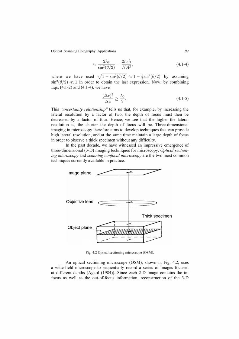
99

¸ œ# #8

Ð Î#Ñ RE

- -

)

! !

# #sin, (4.1-4)

where we have used sin sin by assumingÈ" Ð Î#Ñ ¸ " Ð Î#Ñ# "#

#) )

sin in order to obtain the last expression. Now, by combining#Ð Î#Ñ ¥ ")Eqs. (4.1-2) and (4.1-4), we have

. (4.1-5)Ð <Ñ

D #

? -

?

#!

This tells us that, for example, by increasing theuncertainty relationshiplateral resolution by a factor of two, the depth of focus must then bedecreased by a factor of four. Hence, we see that the higher the lateralresolution is, the shorter the depth of focus will be. Three-dimensionalimaging in microscopy therefore aims to develop techniques that can providehigh lateral resolution, and at the same time maintain a large depth of focusin order to observe a thick specimen without any difficulty. In the past decade, we have witnessed an impressive emergence of

Fig. 4.2 Optical sectioning microscope (OSM).

“ ”

three-dimensional (3-D) imaging techniques for microscopy. Optical section-ing microscopy and scanning confocal microscopy are the two most commontechniques currently available in practice.

a wide-field microscope to sequentially record a series of images focusedAn optical sectioning microscope (OSM), shown in Fig. 4.2, uses

at different depths [Agard (1984)]. Since each 2-D image contains the in-focus as well as the out-of-focus information, reconstruction of the 3-D


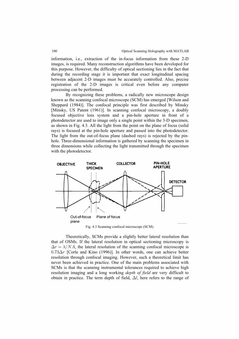
100

information, i.e., extraction of the in-focus information from these 2-Dimages, is required. Many reconstruction algorithms have been developed forthis purpose. However, the difficulty of optical sectioning lies in the fact thatduring the recording stage it is important that exact longitudinal spacingbetween adjacent 2-D images must be accurately controlled. Also, preciseregistration of the 2-D images is critical even before any computerprocessing can be performed. By recognizing these problems, a radically new microscope designknown as the scanning confocal microscope (SCM) has emerged [Wilson andSheppard (1984)]. The confocal principle was first described by Minsky[Minsky, US Patent (1961)]. In scanning confocal microscopy, a doublyfocused objective lens system and a pin-hole aperture in front of aphotodetector are used to image only a single point within the 3-D specimen,as shown in Fig. 4.3. All the light from the point on the plane of focus (solidrays) is focused at the pin-hole aperture and passed into the photodetector.The light from the out-of-focus plane (dashed rays) is rejected by the pin-hole. Three-dimensional information is gathered by scanning the specimen inthree dimensions while collecting the light transmitted through the specimenwith the photodetector.

Fig. 4.3 Scanning confocal microscope (SCM).

Theoretically, SCMs provide a slightly better lateral resolution thanthat of OSMs. If the lateral resolution in optical sectioning microscopy is? -< œ ÎRE, the lateral resolution of the scanning confocal microscope is!Þ($ <? [Corle and Kino (1996)]. In other words, one can achieve betterresolution through confocal imaging. However, such a theoretical limit hasnever been achieved in practice. One of the main problems associated withSCMs is that the scanning instrumental tolerances required to achieve highresolution imaging and a long working are very difficult todepth of field obtain in practice. The term depth of field, , here refers to the range of?6


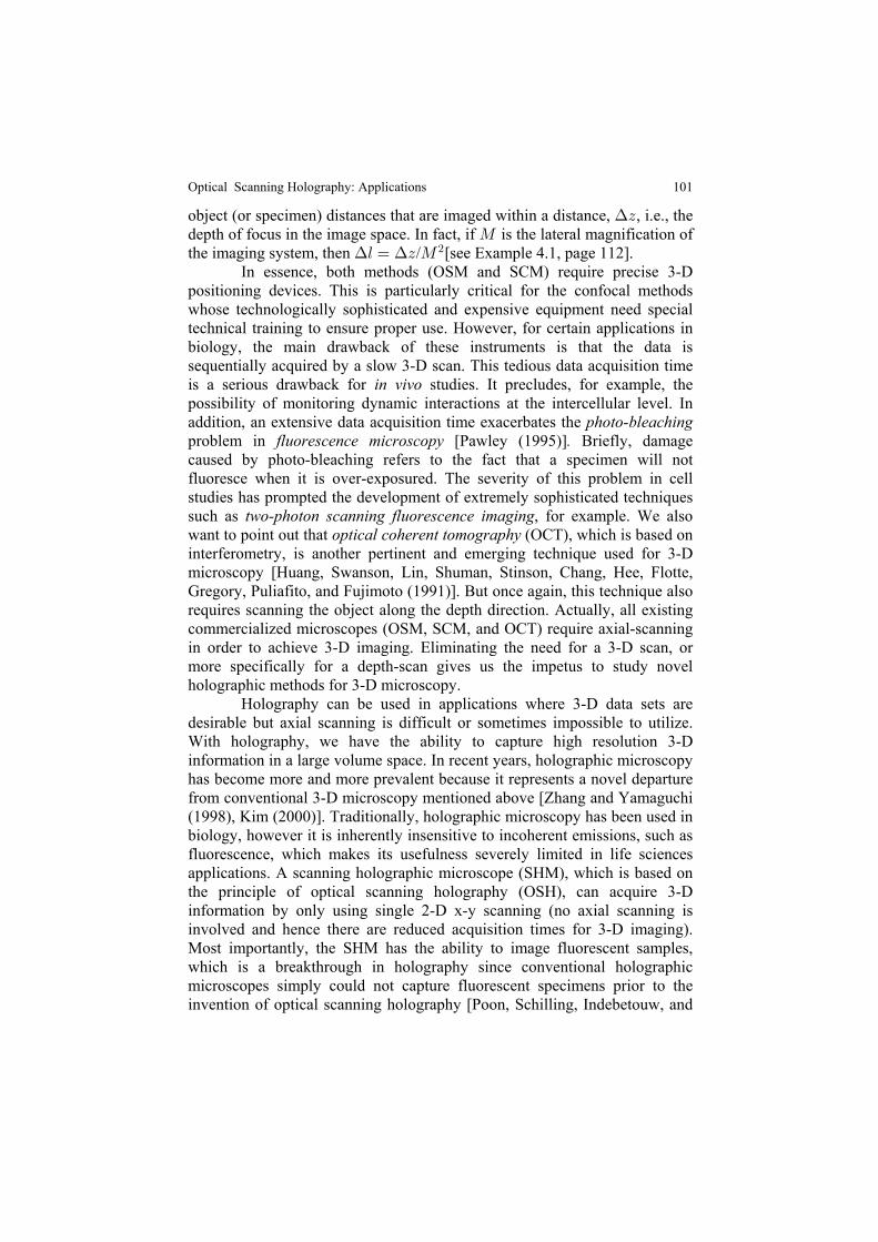
101

object (or specimen) distances that are imaged within a distance, , i.e., the?Ddepth of focus in the image space. In fact, if is the lateral magnification ofQthe imaging system, then / [see Example 4.1, page 112].? ?6 œ D Q#

In essence, both methods (OSM and SCM) require precise 3-Dpositioning devices. This is particularly critical for the confocal methodswhose technologically sophisticated and expensive equipment need specialtechnical training to ensure proper use. However, for certain applications inbiology, the main drawback of these instruments is that the data issequentially acquired by a slow 3-D scan. This tedious data acquisition timeis a serious drawback for studies. It precludes, for example, thein vivopossibility of monitoring dynamic interactions at the intercellular level. Inaddition, an extensive data acquisition time exacerbates the photo-bleachingproblem in Briefly, damagefluorescence microscopy . [Pawley (1995)]caused by photo-bleaching refers to the fact that a specimen will notfluoresce when it is over-exposured. The severity of this problem in cellstudies has prompted the development of extremely sophisticated techniquessuch as , for example. We alsotwo-photon scanning fluorescence imagingwant to point out that (OCT), which is based onoptical coherent tomographyinterferometry, is another pertinent and emerging technique used for 3-Dmicroscopy [Huang, Swanson, Lin, Shuman, Stinson, Chang, Hee, Flotte,Gregory, Puliafito, and Fujimoto (1991)]. But once again, this technique alsorequires scanning the object along the depth direction. Actually, all existingcommercialized microscopes (OSM, SCM, and OCT) require axial-scanningin order to achieve 3-D imaging. Eliminating the need for a 3-D scan, ormore specifically for a depth-scan gives us the impetus to study novelholographic methods for 3-D microscopy. Holography can be used in applications where 3-D data sets aredesirable but axial scanning is difficult or sometimes impossible to utilize.With holography, we have the ability to capture high resolution 3-Dinformation in a large volume space. In recent years, holographic microscopyhas become more and more prevalent because it represents a novel departurefrom conventional 3-D microscopy mentioned above [Zhang and Yamaguchi(1998), Kim (2000)]. Traditionally, holographic microscopy has been used inbiology, however it is inherently insensitive to incoherent emissions, such asfluorescence, which makes its usefulness severely limited in life sciencesapplications. A scanning holographic microscope (SHM), which is based onthe principle of optical scanning holography (OSH), can acquire 3-Dinformation by only using single 2-D x-y scanning (no axial scanning isinvolved and hence there are reduced acquisition times for 3-D imaging).Most importantly, the SHM has the ability to image fluorescent samples,which is a breakthrough in holography since conventional holographicmicroscopes simply could not capture fluorescent specimens prior to theinvention of optical scanning holography [Poon, Schilling, Indebetouw, and


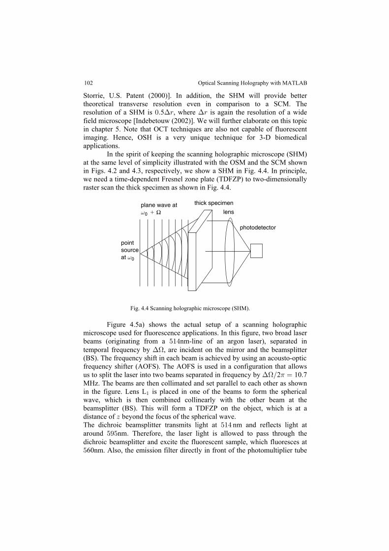
102

Storrie, U.S. Patent (2000)]. In addition, the SHM will provide bettertheoretical transverse resolution even in comparison to a SCM. Theresolution of a SHM is 5 , where is again the resolution of a wide!Þ < <? ?field microscope [Indebetouw (2002)]. We will further elaborate on this topicin chapter 5. Note that OCT techniques are also not capable of fluorescentimaging. Hence, OSH is a very unique technique for 3-D biomedicalapplications. In the spirit of keeping the scanning holographic microscope (SHM)at the same level of simplicity illustrated with the OSM and the SCM shownin Figs. 4.2 and 4.3, respectively, we show a SHM in Fig. 4.4. In principle,we need a time-dependent Fresnel zone plate (TDFZP) to two-dimensionallyraster scan the thick specimen as shown in Fig. 4.4.

Fig. 4.4 Scanning holographic microscope (SHM).

Figure 4.5a) shows the actual setup of a scanning holographicmicroscope used for fluorescence applications. In this figure, two broad laserbeams (originating from a nm-line of an argon laser), separated in&"%temporal frequency by , are incident on the mirror and the beamsplitter?H(BS). The frequency shift in each beam is achieved by using an acousto-opticfrequency shifter (AOFS). The AOFS is used in a configuration that allowsus to split the laser into two beams separated in frequency by 2 10.7?H 1Î œMHz. The beams are then collimated and set parallel to each other as shownin the figure. Lens L is placed in one of the beams to form the spherical"

wave, which is then combined collinearly with the other beam at thebeamsplitter (BS). This will form a TDFZP on the object, which is at adistance of beyond the focus of the spherical wave.DThe dichroic beamsplitter transmits light at nm and reflects light at&"%around nm Therefore, the laser light is allowed to pass through the&*& Þdichroic beamsplitter and excite the fluorescent sample, which fluoresces at&60nm. Also, the emission filter directly in front of the photomultiplier tube

photodetector

thick specimen

lens

pointsourceat ω0

plane wave at 1 Ω


ω0

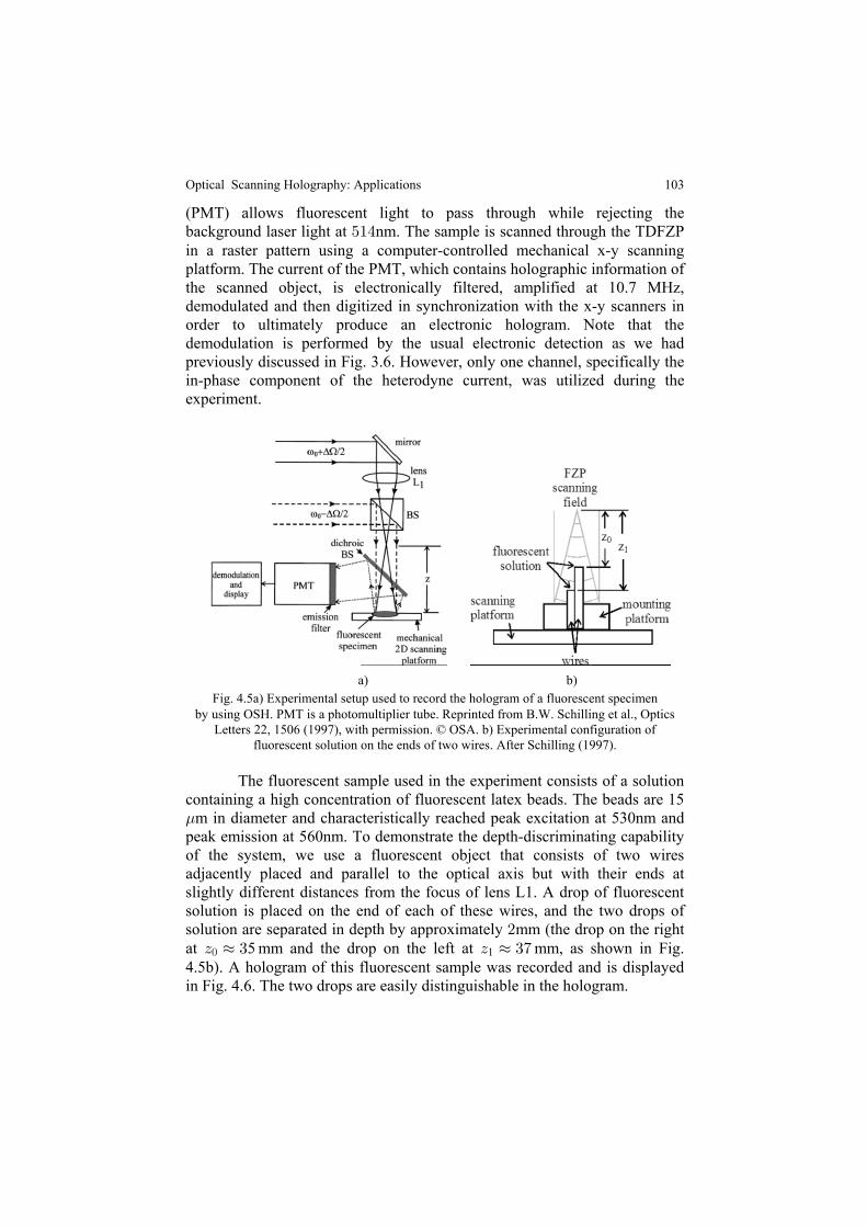
103

(PMT) allows fluorescent light to pass through while rejecting thebackground laser light at nm. The sample is scanned through the TDFZP&"%in a raster pattern using a computer-controlled mechanical x-y scanningplatform. The current of the PMT, which contains holographic information ofthe scanned object, is electronically filtered, amplified at 10.7 MHz,demodulated and then digitized in synchronization with the x-y scanners inorder to ultimately produce an electronic hologram. Note that thedemodulation is performed by the usual electronic detection as we hadpreviously discussed in Fig. 3.6. However, only one channel, specifically the

experiment.

a) b)

Fig. 4.5a) Experimental setup used to record the hologram of a fluorescent specimenby using OSH. PMT is a photomultiplier tube. Reprinted from B.W. Schilling et al., Optics

Letters 22, 1506 (1997), with permission. © OSA. b) Experimental configuration offluorescent solution on the ends of two wires. After Schilling (1997).

The fluorescent sample used in the experiment consists of a solutioncontaining a high concentration of fluorescent latex beads. The beads are 15.m in diameter and characteristically reached peak excitation at 530nm andpeak emission at 560nm. To demonstrate the depth-discriminating capabilityof the system, we use a fluorescent object that consists of two wiresadjacently placed and parallel to the optical axis but with their ends atslightly different distances from the focus of lens L1. A drop of fluorescentsolution is placed on the end of each of these wires, and the two drops ofsolution are separated in depth by approximately mm (the drop on the right#at 5 mm and the drop on the left at mm, as shown in Fig.D ¸ $ D ¸ $(! 14.5b). A hologram of this fluorescent sample was recorded and is displayedin Fig. 4.6. The two drops are easily distinguishable in the hologram.


in-phase component of the heterodyne current, was utilized during the

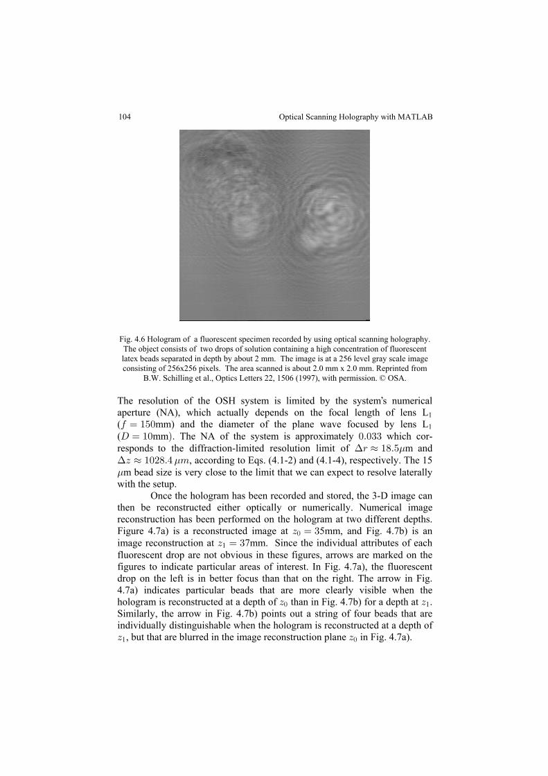
104

Fig. 4.6 Hologram of a fluorescent specimen recorded by using optical scanning holography.The object consists of two drops of solution containing a high concentration of fluorescentlatex beads separated in depth by about 2 mm. The image is at a 256 level gray scale imageconsisting of 256x256 pixels. The area scanned is about 2.0 mm x 2.0 mm. Reprinted from

B.W. Schilling et al., Optics Letters 22, 1506 (1997), with permission. © OSA.

The resolution of the OSH system is limited by the system s numericalaperture (NA), which actually depends on the focal length of lens L1( mm) and the diameter of the plane wave focused by lens L0 œ "&! 1

m and? .D ¸ "!#)Þ% 7, according to Eqs. (4.1-2) and (4.1-4), respectively. The 15.m bead size is very close to the limit that we can expect to resolve laterallywith the setup. Once the hologram has been recorded and stored, the 3-D image canthen be reconstructed either optically or numerically. Numerical imagereconstruction has been performed on the hologram at two different depths.Figure 4.7a) is a reconstructed image at 5mm, and Fig. 4.7b) is anD œ $!

image reconstruction at 7mm. Since the individual attributes of eachD œ $1fluorescent drop are not obvious in these figures, arrows are marked on thefigures to indicate particular areas of interest. In Fig. 4.7a), the fluorescentdrop on the left is in better focus than that on the right. The arrow in Fig.4.7a) indicates particular beads that are more clearly visible when thehologram is reconstructed at a depth of than in Fig. 4.7b) for a depth at .D D! 1Similarly, the arrow in Fig. 4.7b) points out a string of four beads that areindividually distinguishable when the hologram is reconstructed at a depth ofD D1, but that are blurred in the image reconstruction plane in Fig. 4.7a).!

’

(H œ "!mmÑ. The NA of the system is approximately !Þ!$$ which cor-responds to the diffraction-limited resolution limit of ? .< ¸ ")Þ&


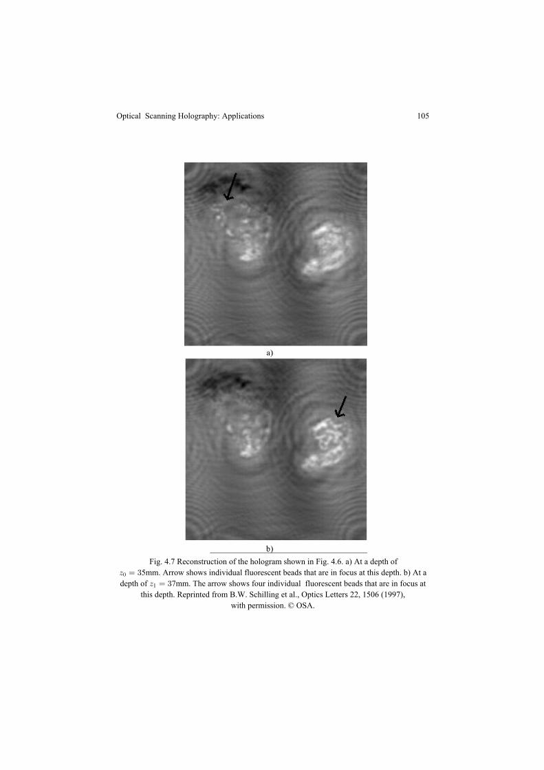
105

Fig. 4.7 Reconstruction of the hologram shown in Fig. 4.6. a) At a depth ofD œ $! 5mm. Arrow shows individual fluorescent beads that are in focus at this depth. b) At adepth of 7mm. The arrow shows four individual fluorescent beads that are in focus atD œ $1

this depth. Reprinted from B.W. Schilling et al., Optics Letters 22, 1506 (1997),with permission. © OSA.


106

Note that since only the in-phase component of the heterodynecurrent has been recorded to create the hologram shown in Fig. 4.6, twin-image noise (residual fringing ) exists in these reconstructions. An important attribute of scanning holographic imaging is that this isthe first time the hologram of a fluorescent specimen has been recorded byusing an optical holographic technique [Poon et al., U.S. Patent (2000)].Holography and fluorescence imaging would never seem to makeconventional sense because holographic techniques require the coherentinterference of light waves and fluorescence imaging does not generatecoherent light. And yet, we have been able to record holograms offluorescent specimens because optical scanning holography makes thispossible. In fact, optical scanning holographic techniques can be applied to3-D biomedical applications as fluorescence imaging [Indebetouw, Kim,Poon, and Schilling (1998)] as well as near-infared imaging [Sun and Xie(2004)] through turbid media have been demonstrated. Most recently a betterthan 1 m-resolution also has been established with a holographic.fluorescence microscope [Indebetouw and Zhong (2006)].

4.2 Three-Dimensional Holographic TV and 3-D Display

Figure 4.8 shows a conceptual holographic system used for 3-D display witha complete recording and reconstruction stages of a point source object. Aswe had mentioned in chapter 2, if the recording film is replaced by, say,some electronic device such as a CCD video camera, then we can create a 3-D display by transferring the CCD s electronic output into some spatial lightmodulator. As we transfer the holographic information at video rate to aspatial light modulator, we create a holographic 3-D display system. The first television transmission of a hologram was demonstrated byEnloe, Murphy, and Rubinstein [1966]. A television camera was used torecord an off-axis hologram where the interference between the Fresneldiffraction pattern of an object transparency and an off-axis plane wave wasrecorded. The recorded hologram was then transmitted over a closed-circuitTV and displayed on a 2-D monitor. The displayed 2-D record was thenphotographed to form a hologram, which was subsequently reconstructed bya coherent optical system. Since then, much progress has been made andmany novel devices have been invented [Macovski (1971), Brown, Nobleand Markevitch, U.S. Patent (1983), Kirk, International Patent (1984),Benton (1991), Shinoda, Suzuki, Wu and Poon, U.S. Patent (1991), Schillingand Poon, U.S. Patent (2004)].

“ ”

’


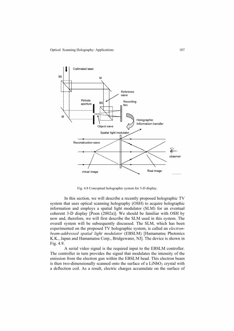
107

Fig. 4.8 Conceptual holographic system for 3-D display.

In this section, we will describe a recently proposed holographic TVsystem that uses optical scanning holography (OSH) to acquire holographicinformation and employs a spatial light modulator (SLM) for an eventualcoherent 3-D display [Poon (2002a)]. We should be familiar with OSH bynow and, therefore, we will first describe the SLM used in this system. Theoverall system will be subsequently discussed. The SLM, which has beenexperimented on the proposed TV holographic system, is called an electron-beam-addressed spatial light modulator (EBSLM) [Hamamatsu PhotonicsK.K., Japan ]. The device is shown inand Hamamatsu Corp., Bridgewater, NJFig. 4.9. A serial video signal is the required input to the EBSLM controller.The controller in turn provides the signal that modulates the intensity of theemission from the electron gun within the EBSLM head. This electron beamis then two-dimensionally scanned onto the surface of a LiNbO crystal with3a deflection coil. As a result, electric charges accumulate on the surface of


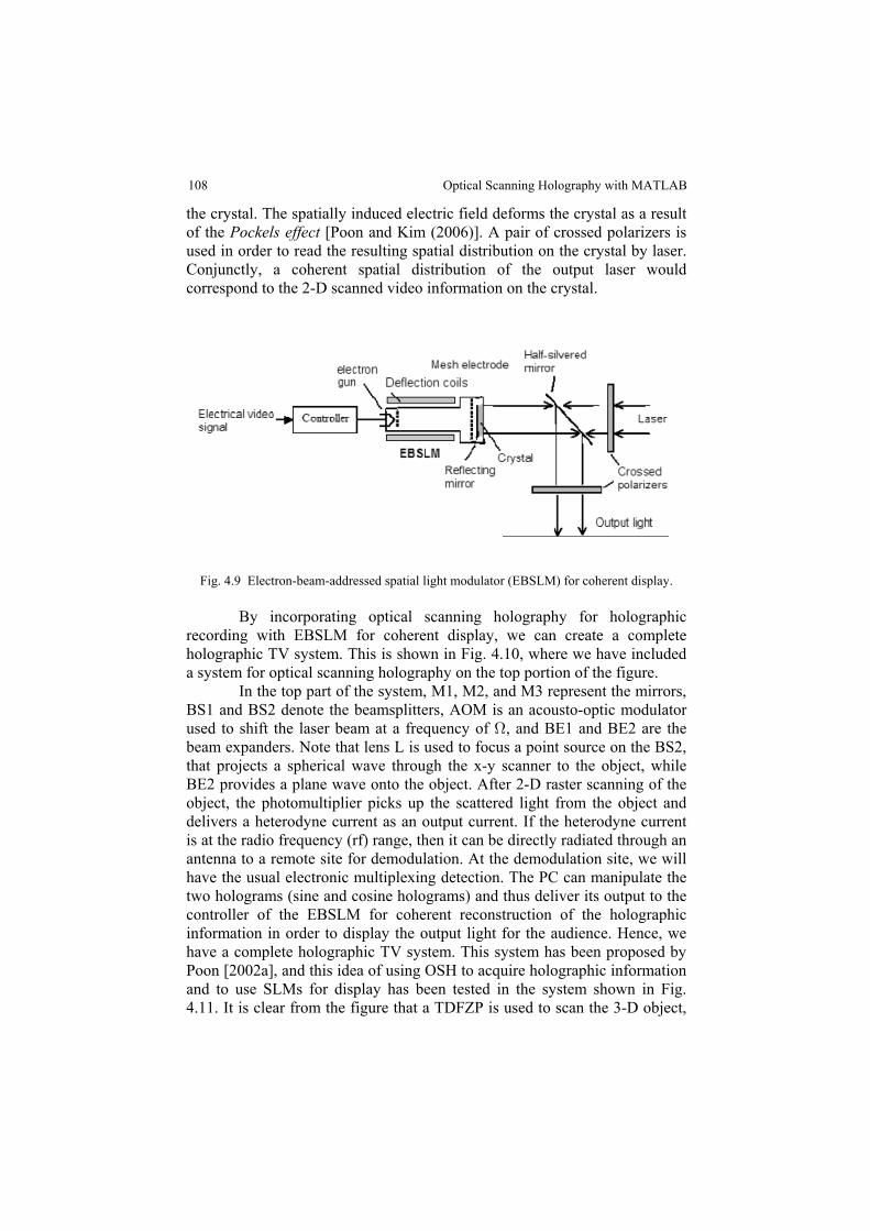
108

the crystal. The spatially induced electric field deforms the crystal as a resultof the [Poon and Kim (2006)]. A pair of crossed polarizers isPockels effect used in order to read the resulting spatial distribution on the crystal by laser.Conjunctly, a coherent spatial distribution of the output laser wouldcorrespond to the 2-D scanned video information on the crystal.

Fig. 4.9 Electron-beam-addressed spatial light modulator (EBSLM) for coherent display.

By incorporating optical scanning holography for holographicrecording with EBSLM for coherent display, we can create a completeholographic TV system. This is shown in Fig. 4.10, where we have includeda system for optical scanning holography on the top portion of the figure. In the top part of the system, M1, M2, and M3 represent the mirrors,BS1 and BS2 denote the beamsplitters, AOM is an acousto-optic modulatorused to shift the laser beam at a frequency of , and BE1 and BE2 are theHbeam expanders. Note that lens L is used to focus a point source on the BS2,that projects a spherical wave through the x-y scanner to the object, whileBE2 provides a plane wave onto the object. After 2-D raster scanning of theobject, the photomultiplier picks up the scattered light from the object anddelivers a heterodyne current as an output current. If the heterodyne currentis at the radio frequency (rf) range, then it can be directly radiated through anantenna to a remote site for demodulation. At the demodulation site, we willhave the usual electronic multiplexing detection. The PC can manipulate thetwo holograms (sine and cosine holograms) and thus deliver its output to thecontroller of the EBSLM for coherent reconstruction of the holographicinformation in order to display the output light for the audience. Hence, wehave a complete holographic TV system. This system has been proposed byPoon [2002a], and this idea of using OSH to acquire holographic informationand to use SLMs for display has been tested in the system shown in Fig.4.11. It is clear from the figure that a TDFZP is used to scan the 3-D object,


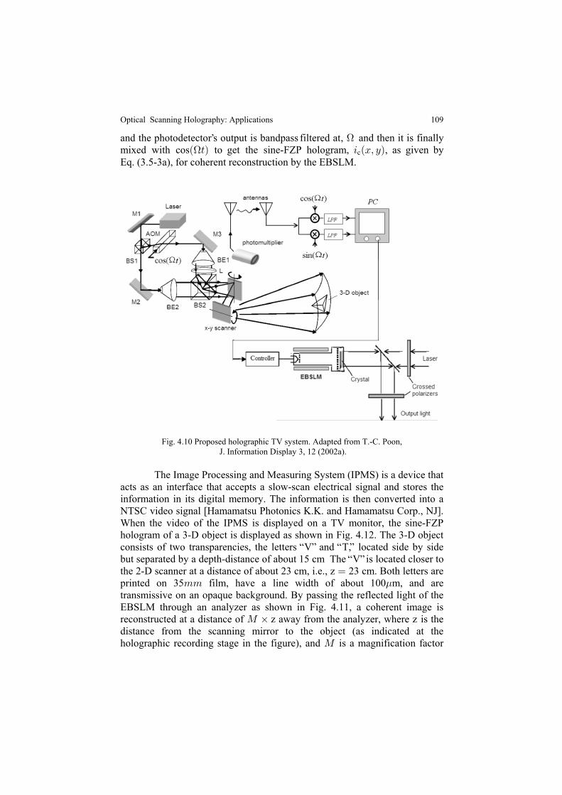
109

c

Fig. 4.10 Proposed holographic TV system. Adapted from T.-C. Poon, J. Information Display 3, 12 (2002a).

The IPMS) is a device thatImage Processing and Measuring System (acts as an interface that accepts a slow-scan electrical signal and stores theinformation in its digital memory. The information is then converted into aNTSC video signal [Hamamatsu Photonics K.K. and Hamamatsu Corp., NJ].When the video of the IPMS is displayed on a TV monitor, the sine-FZPhologram of a 3-D object is displayed as shown in Fig. 4.12. The 3-D objectconsists of two transparencies, the letters V and T, located side by sidebut separated by a depth-distance of about 15 cm The V is located closer tothe 2-D scanner at a distance of about 23 cm, i.e., z 23 cm. Both letters areœprinted on 35 film, have a line width of about 100 m, and are77 .transmissive on an opaque background. By passing the reflected light of theEBSLM through an analyzer as shown in Fig. 4.11, a coherent image isreconstructed at a distance of z away from the analyzer, where z is theQ ‚distance from the scanning mirror to the object (as indicated at theholographic recording stage in the figure), and is a magnification factorQ

’

Eq. (3.5-3a), for coherent reconstruction by the EBSLM.mixed with cosÐ >H Ñ to get the sine-FZP hologram, 3 ÐBß CÑ, as given by

“ ” “ ”“ ”

and the photodetector s output is bandpass filtered at , H and then it is finally


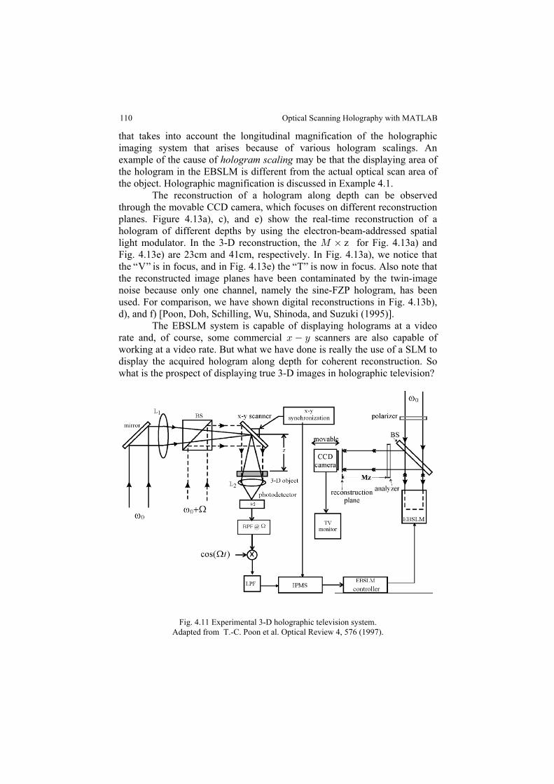
110

that takes into account the longitudinal magnification of the holographicimaging system that arises because of various hologram scalings. Anexample of the cause of may be that the displaying area ofhologram scalingthe hologram in the EBSLM is different from the actual optical scan area ofthe object. Holographic magnification is discussed in Example 4.1. The reconstruction of a hologram along depth can be observedthrough the movable CCD camera, which focuses on different reconstructionplanes. Figure 4.13a), c), and e) show the real-time reconstruction of ahologram of different depths by using the electron-beam-addressed spatiallight modulator. In the 3-D reconstruction, the z for Fig. 4.13a) andQ ‚Fig. 4.13e) are 23cm and 41cm, respectively. In Fig. 4.13a), we notice thatthe V is in focus, and in Fig. 4.13e) the T is now in focus. Also note thatthe reconstructed image planes have been contaminated by the twin-imagenoise because only one channel, namely the sine-FZP hologram, has beenused. For comparison, we have shown digital reconstructions in Fig. 4.13b),d), and f) [Poon, Doh, Schilling, Wu, Shinoda, and Suzuki (1995)]. The EBSLM system is capable of displaying holograms at a videorate and, of course, some commercial scanners are also capable ofB Cworking at a video rate. But what we have done is really the use of a SLM todisplay the acquired hologram along depth for coherent reconstruction. Sowhat is the prospect of displaying true 3-D images in holographic television?

Fig. 4.11 Experimental 3-D holographic television system.Adapted from T.-C. Poon et al. Optical Review 4, 576 (1997).

“ ” “ ”


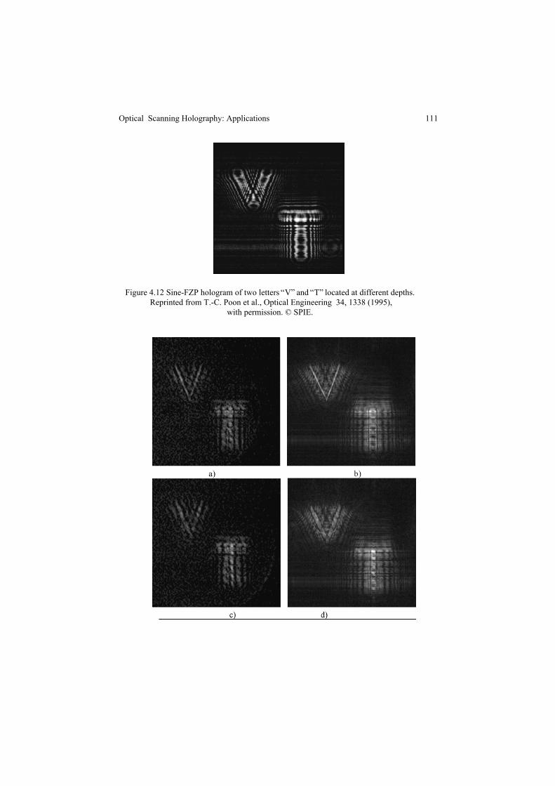
111

Figure 4.12 Sine-FZP hologram of two letters V and T located at different depths. Reprinted from T.-C. Poon et al., Optical Engineering 34, 1338 (1995),

with permission. © SPIE.

“ ” “ ”


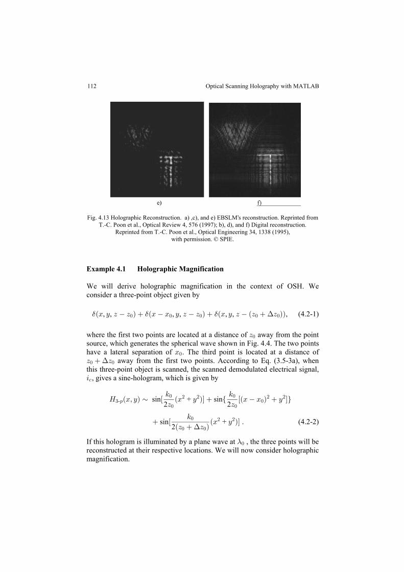
112

Fig. 4.13 Holographic Reconstruction. a) ,c), and e) EBSLM s reconstruction. Reprinted fromT.-C. Poon et al., Optical Review 4, 576 (1997); b), d), and f) Digital reconstruction.

Reprinted from T.-C. Poon et al., Optical Engineering 34, 1338 (1995),with permission. © SPIE.

Example 4.1 Holographic Magnification

We will derive holographic magnification in the context of OSH. Weconsider a three-point object given by

, , , , , , , (4.2-1)$ $ $ ?ÐB C D D Ñ ÐB B C D D Ñ ÐB C D ÐD D ÑÑ! ! ! ! !

where the first two points are located at a distance of away from the pointD!source, which generates the spherical wave shown in Fig. 4.4. The two pointshave a lateral separation of . The third point is located at a distance ofB!

D D! !? away from the first two points. According to Eq. (3.5-3a), whenthis three-point object is scanned, the scanned demodulated electrical signal,3-, gives a sine-hologram, which is given by

L ÐBß CÑ μ Ò ÐB C ÑÓ Ö ÒÐB B Ñ C Ó×5 5

D D$ : !

! !

! !

# # # #- sin + sin

2 2

sin + . (4.2-2)2

Ò ÐB C ÑÓ5

ÐD D Ñ!

! !

# #

?

If this hologram is illuminated by a plane wave at , the three points will be-!

reconstructed at their respective locations. We will now consider holographicmagnification.

’


113

a) Hologram Scaling

Magnification can be achieved by enlarging holograms, however, it is adifficult task especially when we deal with off-axis holograms where fringedensities are of the order of several thousands lp/mm. Most photographicenlargers do not have a sufficient resolution in order to handle these details.Hence, the method is not very practical. With the scanning technique,however, on-axis holograms are generated and scaling is straightforward.The hologram can be scaled by a factor of , simply by displaying theQhologram in an area that is different from the optical scan area. In this case,Eq. (4.2-2) becomes

L ÐQB QCÑ œ Ö ÒÐQBÑ ÐQCÑ Ó×5

D$ :

!

!

# #- , sin

2

Ö ÒÐQB B Ñ ÐQCÑ Ó×5

Dsin

2!

!!

# #

Ö ÒÐQBÑ ÐQCÑ Ó×5

ÐD D Ñsin . (4.2-3)

2!

! !

# #

?

When <1, we have magnification, whereas >1 corresponds toQ Qdemagnification. By re-writing Eq. (4.2-3), we have

L ÐQB QCÑ œ Ò ÐB C ÑÓ5

D Q$ :

!

!#

# #- , sin

2 /

Ö ÒÐB B QÑ C Ó× Ö ÐB C Ñ×5 5

D Q ÐD D Ñ Qsin / sin .

2 / 2 /! !

! ! !# #!

# # # #

?

(4.2-4) Now, during optical reconstruction using a wavelength , we see-!

that by inspection of the first and second term in Eq. (4.2-4), the two realimage points are now formed at a distance of / away from theD Q!

#

hologram, and with a reconstructed lateral distance of / away from eachB Q!

other. By defining the , M , as the ratio of thelateral magnification latreconstructed lateral distance to the original lateral distance, , we haveB!

M 1/ . In order to determine the magnification along the longitudinallat œ Qdirection, we must focus on the first and the third terms, and uponreconstruction, we see that the two points are reconstructed at / andD Q!

#

( )/ , respectively. By defining the ,D D Q! !#? longitudinal magnification

M , as the ratio of the reconstructed longitudinal distance, / , to thelong ?D Q!#

original longitudinal distance, , we have M =1/ .?D Q!#

long


114

b) Wavelength Scaling

We could reconstruct the hologram with a different wavelength, say m (or-!

5!/m), where m is a constant. Hence, according to Fresnel diffraction, thefield distribution at away from the hologram is now given byD

L ÐB CÑ ‡ 2ÐB C D 5 Ñ$ : !- , , ; , /m

º Ò ÐB C ÑÓ Ö ÒÐB B Ñ C Ó×5 5

D Dšsin sin

2 2! !

! !

# # # #!

Ò ÐB C ÑÓ ‡ Ò ÐB C ÑÓ5 45 45

ÐD D Ñ D Dsin + exp .

2 2 2/m /m! ! !

! !

# # # #

? 1›

(4.2-5)

This equation suggests that there will be no magnification in the lateraldirection. Along the longitudinal direction, we can inspect the results of thefirst and the third terms. And again when we consider real imagereconstruction, the first and the second term will form an image at /m.D œ D!The third term gives rise to a real image at )/m. Hence, in thisD œ ÐD D! !?case M 1, and M 1/m. The reconstructed volume is eitherlat longœ œcompressed or expanded by a factor of 1/m with the same lateralmagnification. When m>1, we have compression. With visible light forrecording and reconstruction, m is in the range of 0.5 to 1.8. However, whenusing digital reconstruction, m can be arbitrarily chosen.

c) Reconstruction combining hologram scaling and wavelength scaling

If we change the scale of the hologram and use a different wavelength forreconstruction, then the combined magnification along the lateral andlongitudinal direction will be M 1/ and M 1/m . Therefore,lat longœ Q œ Q#

we see that the reconstructed volume, /m , is different from theB D Q! !$?

original volume . This creates distortion when we magnify the originalB D! !?3-D object. This is a well-known result of magnification in 3-D opticalimaging. In order to have a true 3-D perspective on reconstruction, when thescale change of the hologram is given by , we let m 1/ which gives usQ œ QM m and M m, and therefore, we obtain M M . In otherlat long lat longœ œ œwords, in order to prevent distortion in 3-D imaging, we scale the hologramby a factor , and then the reconstructing wavelength should be m , whereQ -!

-! is the recording wavelength and m is equal to 1/ . This is the originalQidea of Gabor [1949] who first conceptualized the notion during the pre-laserera to improve upon the electron microscope. Electron microscopy was themotivational factor in the development of holography.


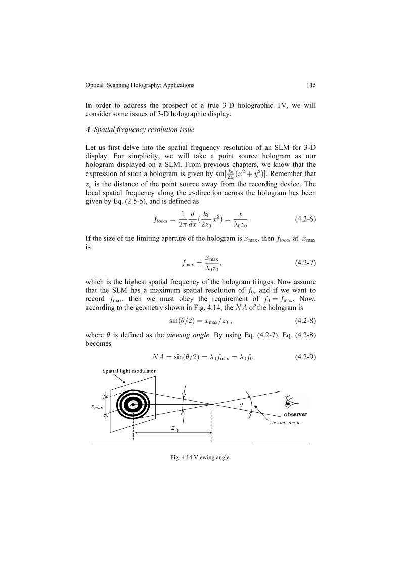
115

In order to address the prospect of a true 3-D holographic TV, we willconsider some issues of 3-D holographic display.

A. Spatial frequency resolution issue

Let us first delve into the spatial frequency resolution of an SLM for 3-Ddisplay. For simplicity, we will take a point source hologram as ourhologram displayed on a SLM. From previous chapters, we know that theexpression of such a hologram is given by sin . Remember thatÒ ÐB C ÑÓ5

#D# #!

!

D! is the distance of the point source away from the recording device. Thelocal spatial frequency along the -direction across the hologram has beenBgiven by Eq. (2.5-5), and is defined as

0 œ Ð B Ñ œ" . 5 B

# .B D D69-+6

!

! ! !

#

1 -2. (4.2-6)

If the size of the limiting aperture of the hologram is , then B Bmax max069-+6 at is

0 œD

maxBmax

-! !, (4.2-7)

which is the highest spatial frequency of the hologram fringes. Now assumethat the SLM has a maximum spatial resolution of , and if we want to0!record , then we must obey the requirement of . Now,0 0 œ 0max max!

according to the geometry shown in Fig. 4.14, the of the hologram isRE

sinÐ Î#Ñ œ) B ÎDmax ! , (4.2-8)

where sing Eq. (4.2-7), Eq. (4.2-8)) is defined as the . By uviewing anglebecomes

(4.2-9)RE œ sin . Ð Î#Ñ œ 0 œ 0) - -! ! !max

Fig. 4.14 Viewing angle.


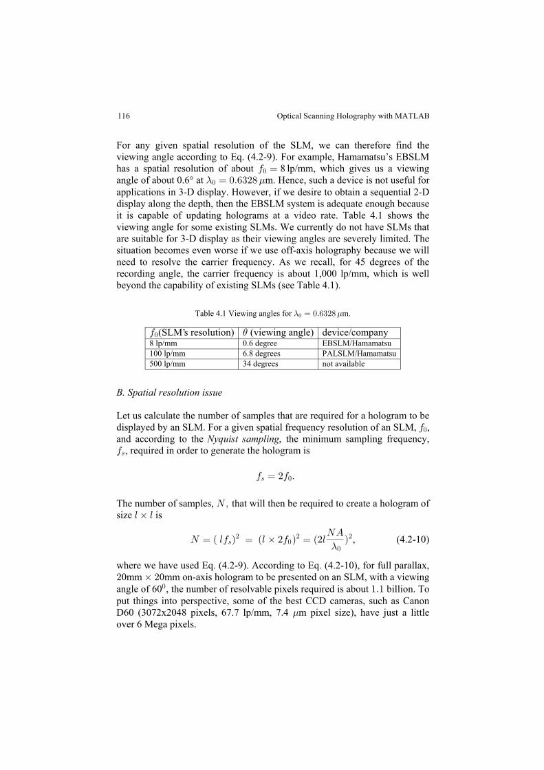
116

For any given spatial resolution of the SLM, we can therefore find theviewing angle according to Eq. (4.2-9). For example, Hamamatsu’s EBSLMhas a spatial resolution of about 8 lp/mm, which gives us a viewing0 œ!

angle of about 0.6° at . Hence, such a device is not useful for- .! œ !Þ'$#) mapplications in 3-D display. However, if we desire to obtain a sequential 2-Ddisplay along the depth, then the EBSLM system is adequate enough becauseit is capable of updating holograms at a video rate. Table 4.1 shows theviewing angle for some existing SLMs. We currently do not have SLMs thatare suitable for 3-D display as their viewing angles are severely limited. Thesituation becomes even worse if we use off-axis holography because we willneed to resolve the carrier frequency. As we recall, for 45 degrees of therecording angle, the carrier frequency is about 1,000 lp/mm, which is wellbeyond the capability of existing SLMs (see Table 4.1).

Table 4.1 Viewing angles for .- .! œ !Þ'$#) m

0!(SLM s resolution) (viewing angle))8 lp/mm 0.6 degree EBSLM/Hamamatsu100 lp/mm 6.8 degrees PALSLM/Hamamatsu500 lp/mm 34 degrees not available

B. Spatial resolution issue

,

0=, required in order to generate the hologram is

0 œ #= 0!.

The number of samples, that will then be required to create a hologram ofRßsize 6 ‚ 6 is

R œ Ð 6 Ñ œ Ð6 ‚ # Ñ œ Ð#6 ÑRE

, (4.2-10)0=# # #0!

! -

where we have used Eq. (4.2-9). According to Eq. (4.2-10), for full parallax,# ‚ #0mm 0mm on-axis hologram to be presented on an SLM, with a viewingangle of 60 , the number of resolvable pixels required is about billion. To! "Þ"put things into perspective, some of the best CCD cameras, such as CanonD60 (3072x2048 pixels, 67.7 lp/mm, 7.4 m pixel size), have just a little.over 6 Mega pixels.

’

!displayed by an SLM. For a given spatial frequency resolution of an SLM, 0

device/company

Let us calculate the number of samples that are required for a hologram to be

and according to the Nyquist sampling, the minim um sampling frequency,


117

C. Data transmission issue

As we had previously calculated, a single frame of a 0mm 0mm# ‚ #hologram with a viewing angle of 60° requires about 1.1 billion pixels on theSLM. To update such a frame with an 8-bit resolution at 30 frames/s, a serialdata rate of

1.1 billion samples/frame 8 bits/sample 30 frames/s 0.26 Tbit/s‚ ‚ œ

is required for full parallax. Basically, all the issues that we have discussed illustrate the fact thatcontent of information held within a hologram is enormous. This implies thatthe content of information in the hologram must be significantly reduced inorder to achieve 3-D holographic TV for 3-D display. Live 3-D TV withholographic images is truly a formidable problem. However, since we areused to looking at the world with our two eyes more or less on a horizontallevel, we are usually satisfied with horizontal parallax. Hence, for 512vertical lines, the number of pixels required becomes ,&"# ‚ Ð#6 ‚ #REÎ Ñ-!

which is approximately 17 million, if we are to eliminate vertical parallax.By scarifying vertical parallax, the data rate becomes 4 Gbits per secondinstead of 0.26 Tbits per second, which is calculated for full parallax. Andthis is manageable with advanced modern optical communications systems.

real-world applications. The possibility of real-time holographic TV becomes

Optical scanning holography with horizontal-parallax-only recordingis possible if we scan the object with a 1-D TDFZP. This idea, called HPO-optical scanning holography, has been proposed recently while computersimulations have been performed [Poon, Akin, Indebetouw, and Kim (2005),Poon (2006)].

4.3 Optical Scanning Cryptography

Due to the recent progress in the development of optical components and theincreased technical performance of optical systems, optical cryptography has

By using fiber optics, data rates of up to 40 Gbit/s indeed can be achieved in

a reality if the horizontal-parallax-only (HPO)-electronic holographic recor-ding technique becomes available. Indeed, by using computer-generated,horizontal-parallax-only holographic information, the MIT group has demon-strated a 3-D holographic display having 64 vertical lines and with viewingangle of about 15 degrees [St. Hilaire, Benton, Lucente, Jepsen, Kollin, Yoshikawa, Underkoffler (1990), St. Hilaire, Benton, and Lucente (1992)].However, this HPO-holographic information is computer generated and noHPO-holographic information has actually been generated by or recordedfrom actual real objects.


118

a significant potential in advances for security applications. Indeed there hasbeen a plethora of articles that deal with secure systems that use opticalmethods [Lohmann, Stork, and Stucke (1986), Refregier and Javidi (1995),Lai and Neifeld (2000), Wang, Sun, Su, and Chiou (2000), Magensen andGluckstad (2001)]. One of the reasons for using optical encryption is thatinformation, such as images, that needs to be encrypted exists already in theoptical domain. Another reason is that optical encryption, as opposed toelectronic or digital encryption, can provide many degrees of freedom whensecuring sensitive information. When large volumes of information need tobe encrypted, such as a 3-D object, using optical encryption methods isprobably the most logical choice. Although most optical encryptiontechniques are typically coherent, some incoherent optical techniques forencryption have recently been proposed [Tajahuerce, Lancis, Javidi, andAndres (2001)]. In general, incoherent optical techniques have manyadvantages over their coherent counterparts. This includes a better S/N ratioand insensitivity to the misalignment of optical elements. In this section, wewill discuss an incoherent optical method based on optical scanningholography for encryption. This method is called optical scanningcryptography (OSC) [Poon, Kim, and Doh (2003)]. While having thecapability to utilize incoherent processing, the method also has many otheradvantages. These advantages include the following. 1) Since it is an opticalscanning method, it can process incoherent objects, such as printeddocuments, without using a spatial light modulator (SLM) to convert anincoherent image into a coherent image as existing coherent techniquescurrently do. The proposed system can indeed perform real-time or on-the-flyencryption. 2) Since the output signal is a heterodyne electrical signal, andhence the encrypted information is riding on a heterodyne frequency (or acarrier frequency as used in communications), it can immediately be radiatedfor wireless transmission to a secure site for storage and then subsequently beencrypted. This may have important applications in radio frequencyidentification RFID( ) [Radio Frequency Identification Technologies: AWorkshop Summary (2004)]. 3) Because the technique is based onholography, it can be easily extended to the use of encrypting 3-Dinformation. Figure 4.15 shows the optical system utilized for encryption anddecryption. The system contains two subsystems: an encryption stage and adecryption stage. It is noted that the two subsystems have an identical two-pupil optical heterodyne scanning image processor, which we haveextensively studied in section 3.4. We will first briefly summarize theprevious results of the image processor, and then we will discuss encryptionand decryption.


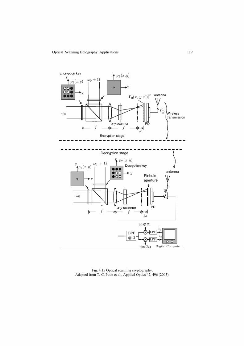
119

Fig. 4.15 Optical scanning cryptography.Adapted from T.-C. Poon et al., Applied Optics 42, 496 (2003).


Decryption stage

Pinholeaperture

antenna

PDx-y scanner

Decryption key1

2ω0 + W

ω0

f fzd

xx

yy

ic

isBPF@ W

LPF

LPF

Digital Computer

cos(Wt)

sin(Wt)

Encryption key

Encryption stage

antenna

Wirelesstransmission

PDx-y scanner

p1

2

Γ0(x, y; zc)

ω0 + W

ω0

f fzc

x

x

yy

icW

p (x,y)

p (x,y)

p (x,y)(x,y)

2

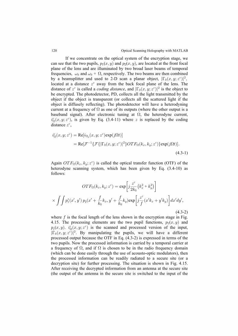
120

If we concentrate on the optical system of the encryption stage, wecan see that the two pupils, , are located at the front focal: Bß CÑ : Bß CÑ" #( and (plane of the lens and are illuminated by two broad laser beams of temporalfrequencies, and + , respectively. The two beams are then combined= = H! !

by a beamsplitter and used to 2-D scan a planar object, l ÐBß Cà D Ñl ß>!- #

located at a distance away from the back focal plane of the lens. TheD-

distance of is called a , and is the object toD l ÐBß Cà D Ñl- - #!coding distance >

be encrypted. The photodetector, PD, collects all the light transmitted by theobject if the object is transparent (or collects all the scattered light if theobject is diffusely reflecting). The photodetector will have a heterodyningcurrent at a frequency of as one of its outputs (where the other output is aHbaseband signal). After electronic tuning at , the heterodyne current,H3 ÐBß Cà D Ñ D- -H , is given by Eq. (3.4-11) where is replaced by the coding

distance ,D-

Re exp3 ÐBß Cà D Ñ œ Ò3 ÐBß Cà D Ñ Ð4 >ÑÓ- - -H H: H

Re exp .œ Ò Ö Öl ÐBß Cà D Ñl ×SXJ Ð5 ß 5 à D Ñ× Ð4 >ÑÓY Y > H" - # -! B CH

(4.3-1)

Again is called the optical transfer function (OTF) of theSXJ Ð5 ß 5 à D ÑH B C-

heterodyne scanning system, which has been given by Eq. (3.4-10) asfollows:

SXJ Ð5 ß 5 à D Ñ œ 4 5 5D

#5H B C

- # #-

!B Cexp + ” •ˆ ‰

‚ : ÐB C Ñ : ÐB 5 C 5 Ñ 4 ÐB 5 C 5 Ñ .B .C0 0 D

5 5 0( ( ” •‡ w w w w w w w w

" #! !

B C B C

-

, , exp ,

(4.3-2)where is the focal length of the lens shown in the encryption stage in Fig.04.15. The processing elements are the two pupil functions, ( and: Bß CÑ"

: Bß CÑ 3 ÐBß Cà D Ñ#( . - -H is the scanned and processed version of the input,

l ÐBß Cà D Ñl Þ>!- # By manipulating the pupils, we will have a different

processed output because the OTF in Eq. (4.3-2) is expressed in terms of thetwo pupils. Now the processed information is carried by a temporal carrier ata frequency of , and if is chosen to be in the radio frequency domainH H(which can be done easily through the use of acousto-optic modulators), thenthe processed information can be readily radiated to a secure site (or adecryption site) for further processing. The situation is shown in Fig. 4.15.After receiving the decrypted information from an antenna at the secure site(the output of the antenna in the secure site is switched to the input of the


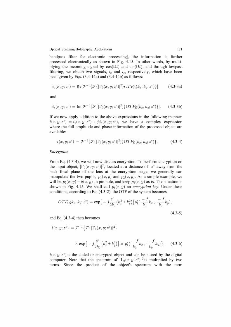
121

bandpass filter for electronic processing), the information is further

- =

been given by Eqs. (3.4-14a) and (3.4-14b) as follows:

3 ÐBß Cà D Ñ œ Ö Öl ÐBß Cà D Ñl ×SXJ Ð5 ß 5 à D Ñ× Ð Ñ- ! B C- " - # -Re 4.3-3ac dY Y > H

and

3 ÐBß Cà D Ñ œ Ö Öl ÐBß Cà D Ñl Ñ×SXJ Ð5 ß 5 à D Ñ× Þ Ð= ! B C- " - # -Im 4.3-3b)c dY Y > H

If we now apply addition to the above expressions in the following manner:3ÐBß Cà D Ñ œ 3 ÐBß Cà D Ñ 4 3 ÐBß Cà D Ñ- - -

- = , we have a complex expressionwhere the full amplitude and phase information of the processed object areavailable:

. (4.3-4)3ÐBß Cà D Ñ œ Ö Öl ÐBß Cà D Ñl Ñ×SXJ Ð5 ß 5 à D Ñ×- " - # -! B CY Y > H

Encryption

From Eq. (4.3-4), we will now discuss encryption. To perform encryption onthe input object, , located at a distance of away from thel ÐBß Cà D Ñl D>!

- # -

back focal plane of the lens at the encryption stage, we generally canmanipulate the two pupils, and . As a simple example, we: ÐBß CÑ : ÐBß CÑ1 2will let = , a pin hole, and keep as is. The situation is: ÐBß CÑ ÐBß CÑ : ÐBß CÑ2 $ "

shown in Fig. 4.15. We shall call ( an Under these: Bß CÑ" encryption key. conditions, according to Eq. (4.3-2), the OTF of the system becomes

SXJ 5 ß 5 à D œ 4 5 5 : Ð 5 5 ÑD 0 0

#5 5 5H( ) exp + , , B C B C

- # # ‡-

! ! !B C "

ˆ ‰‘(4.3-5)

and Eq. (4.3-4) then becomes

3ÐBß Cà D Ñ œ Öl ÐBß Cà D Ñl ×- " - #!Y Y >˜

‚ 4 5 5 ‚ : Ð 5 5 ÑD 0 0

#5 5 5exp + , . (4.3-6) ˆ ‰‘ ™-

! ! !

# # ‡B C " B C

3 Bß Cà Da b- is the coded or encrypted object and can be stored by the digitalcomputer. Note that the spectrum of is multiplied by twol ÐBß Cà D Ñl>!

- #

terms. Since the product of the object s spectrum with the term

processed electronically as shown in Fig. 4.15. In other words, by multi-plying the incoming signal by cosa bH H> > and sina b, and through lowpassfiltering, we obtain two signals, 3 and 3 , respectively, which have been

’


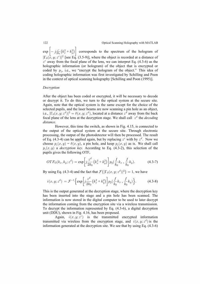
122

exp + corresponds to the spectrum of the hologram ofˆ ‰ 4 5 5D#5

# #B C

-

!

l ÐBß Cà D Ñl>!- # [see Eq. (3.5-9)], where the object is recorded at a distance of

D- away from the focal plane of the lens, we can interpret Eq. (4.3-6) as theholographic information (or hologram) of the object that is encrypted orcoded by , i.e., we encrypt the hologram of the object. This idea of:"coding holographic information was first investigated by Schilling and Poonin the context of optical scanning holography [Schilling and Poon (1995)].

Decryption

After the object has been coded or encrypted, it will be necessary to decodeor decrypt it. To do this, we turn to the optical system at the secure site.Again, note that the optical system is the same except for the choice of theselected pupils, and the laser beams are now scanning a pin hole as an object,i.e., , located at a distance away from the backl ÐBß Cà D Ñl œ ÐBß Cà D Ñ D> $!

. # . .

focal plane of the lens at the decryption stage. We shall call the D. decodingdistance. However, this time the switch, as shown in Fig. 4.15, is connected tothe output of the optical system at the secure site. Through electronicprocessing, the output of the photodetector will then be processed. The resultof Eq. (4.3-4) can be applied again, but by replacing with by . Now weD D- .

choose = , a pin hole, and keep as is. We shall call: ÐBß CÑ ÐBß CÑ : ÐBß CÑ" #$: ÐBß CÑ# a . According to Eq. (4.3-2), this selection of the decryption keypupils gives the following OTF,

SXJ Ð5 ß 5 à D Ñ œ 4 5 5 : Ð 5 5 ÑÞD 0 0

#5 5 5H B C B C

. # #.

! ! !B C #exp + , (4.3-7)” •ˆ ‰

By using Eq. (4.3-4) and the fact that , we haveY >Öl ÐBß Cà D Ñl × œ "!. #

3ÐBß Cà D Ñ œ 4 5 5 : Ð 5 5 ÑD 0 0

#5 5 5. " # #

.

! ! !B C # B CY š ›” •ˆ ‰exp + , . (4.3-8)

This is the output generated at the decryption stage, where the decryption keyhas been inserted into the stage and a pin hole has been scanned. Theinformation is now stored in the digital computer to be used to later decryptthe information coming from the encryption site via a wireless transmission.To decrypt the information represented by Eq. (4.3-6), a digital decryptionunit (DDU), shown in Fig. 4.16, has been proposed. Again, is the transmitted encrypted information3ÐBß Cà D Ñ-

transmitted via wireless from the encryption stage, and is the3ÐBß Cà D Ñ.

information generated at the decryption site. We see that by using Eq. (4.3-6)

“ ”


” •

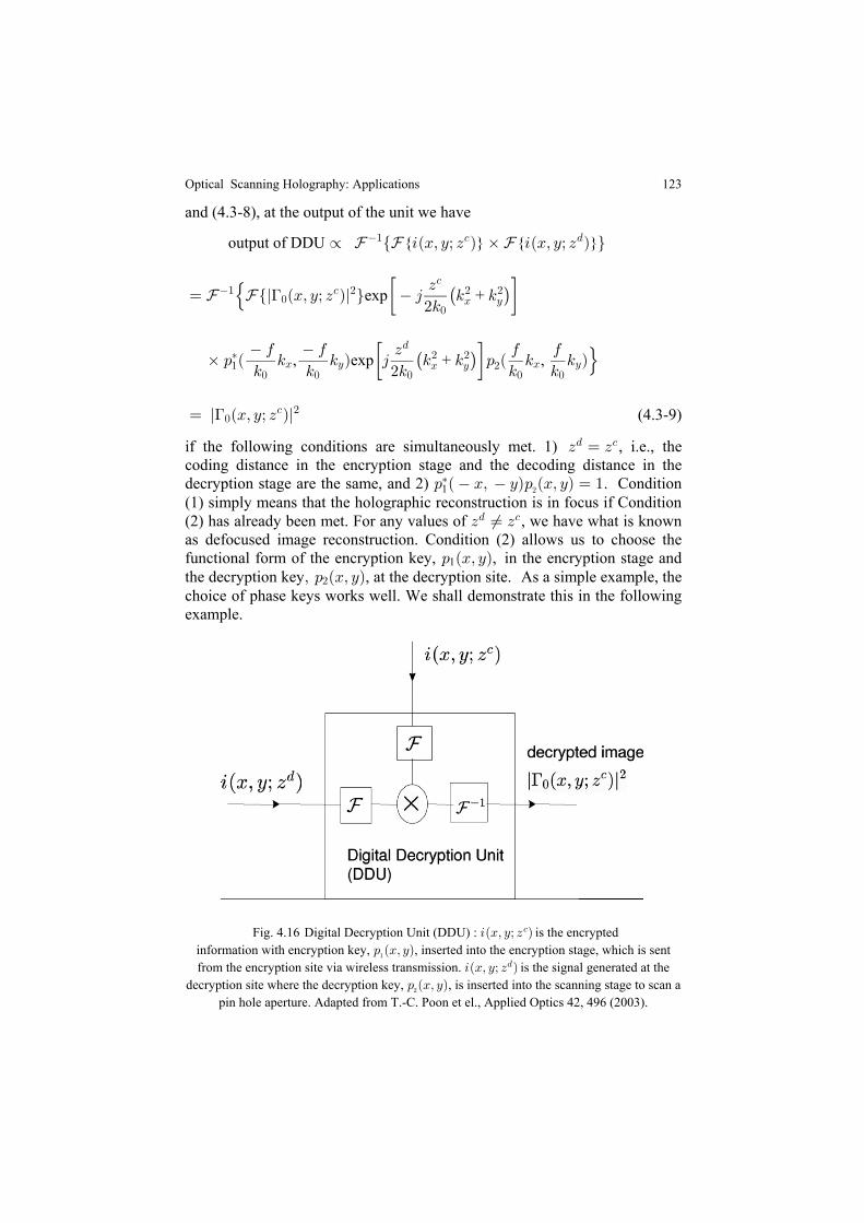
123

and (4.3-8), at the output of the unit we have

output of DDU º Ö 3ÐBß Cà D Ñ ‚ 3ÐBß Cà D Ñ ×Y Y Y" - .

œ Öl ÐBß Cà D Ñl × 4 5 5D

#5Y Y >" - # # #

!

-

!B Cš ” •ˆ ‰exp +

‚ : Ð 5 5 Ñ 4 5 5 : Ð 5 5 Ñ 0 0 D 0 0

5 5 #5 5 5‡ # #" B C #

! ! ! ! !B C B C

.

, exp + , ” •ˆ ‰ ›œ l ÐBß Cà D Ñl (4.3-9)>!

- #

if the following conditions are simultaneously met. 1) , i.e., theD œ D. -

coding distance in the encryption stage and the decoding distance in thedecryption stage are the same, and 2) . Condition: Ð Bß CÑ: ÐBß CÑ œ "‡

1 #

(1) simply means that the holographic reconstruction is in focus if Condition(2) has already been met. For any values of , we have what is knownD Á D. -

as defocused image reconstruction. Condition (2) allows us to choose thefunctional form of the encryption key, , in the encryption stage and: ÐBß CÑ1the decryption key , at the decryption site. As a simple example, theß : ÐBß CÑ#

choice of phase keys works well. We shall demonstrate this in the followingexample.

Fig. 4.16 Digital Decryption Unit (DDU) : 3ÐBß Cà D Ñ- is the encryptedinformation with encryption key, , inserted into the encryption stage, which is sent: ÐBß CÑ

"

from the encryption site via wireless transmission. is the signal generated at the3ÐBß Cà D Ñ.

decryption site where the decryption key, , is inserted into the scanning stage to scan a: ÐBß CÑ#

pin hole aperture. Adapted from T.-C. Poon et el., Applied Optics 42, 496 (2003).


124

Example 4.2 MATLAB Example onOptical Scanning Cryptography

As a simple example, we can immediately see that the choice of a randomphase mask is a good encryption key, i.e., we let exp: ÐBß CÑ œ 4# QÐBß CÑ1 c d1where is a function of random numbers chosen from a uniformQÐBß CÑdistribution between the interval (0.0,1.0). Again, = , i.e., a: ÐBß CÑ ÐBß CÑ2 $pin-hole is the other pupil in the encryption stage. For this choice of pupils,the encrypted image from Eq. (4.3-6) becomes

exp + 3ÐBß Cà D Ñ œ Öl ÐBß Cà D Ñl × 4 5 5D

#5- " - # # #

!

-

!B CY Y >š ” •ˆ ‰

‚ 4# QÐ ß Ñ 05

5 5

05exp . (4.3-10)” •›1

B

! !

C

The above encrypted information can be made more secure if, for example,exp ,Ò4# <ÐBß CÑÓ1

exp 3ÐBß Cà D Ñ œ l ÐBß Cà D Ñl Ò4# <ÐBß CÑÓ- " - #!Y Y > 1š

exp + exp .‚ 4 5 5 4# QÐ ß ÑD 05

#5 5 5

05” • ” •ˆ ‰ ›-

! ! !

# #B C

B C1

(4.3-11)This technique used to obtain the above resulting encrypted image is calleddouble-random phase encoding [Refregier and Javidi (1995)]. We shall useMATLAB in order to simulate this coding. Note that and<ÐBß CÑ QÐBß CÑshould be chosen as two independent random functions. Table 4.2 contains the m-file for the simulations shown in thisexample. Figure 4.17a) shows the original document, . Figurel ÐBß Cà D Ñl>!

- #

4.17b) and 4.17c) show the real part and imaginary part of the originaldocument multiplied by a random phase mask, exp , placedÒ4# <ÐBß CÑÓ1immediately in front of the original document. Figure 4.17d) shows theintensity of the encrypted document, | | , which is calculated using3ÐBß Cà D Ñ-

Eq. (4.3-11) where we have used sigma (zc*ld)/(4*pi) (30)*(0.6*10^-œ œ6)/4 in the m-file [sigma is / in Eq. (4.3-11)].1 D #5-

!

the original document is multiplied by a random phase mask,where <ÐBß CÑ is a function of random numbers. By using Eq. (4.3-10), theoverall encrypted image then becomes

“ ”


125

a) Original document.

b) Real part of the image multiplied by random phase mask.

c) Imaginary part of the image multiplied by random phase mask.


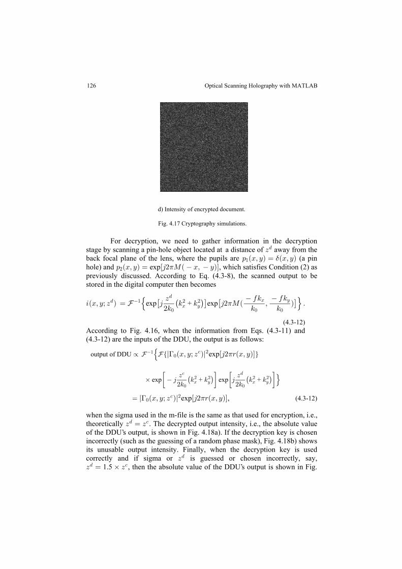
126

d) Intensity of encrypted document.

For decryption, we need to gather information in the decryptionstage by scanning a pin-hole object located at a distance of away from theD.

back focal plane of the lens, where the pupils are (a pin: ÐBß CÑ œ ÐBß CÑ" $hole) and exp , which satisfies Condition (2) as: ÐBß CÑ œ 4# QÐ Bß CÑ# c d1previously discussed. According to Eq. (4.3-8), the scanned output to bestored in the digital computer then becomes

3ÐBß Cà D Ñ œ 4 5 5 4# QÐ ß Ñ ÞD 05

#5 5 5

05. " # #.

! ! !B C

B CY 1š › ˆ ‰‘ ‘exp + exp

(4.3-12)According to Fig. 4.16, when the information from Eqs. (4.3-11) and(4.3-12) are the inputs of the DDU, the output is as follows:

output of DDU º Ö ×Y Y"š l ÐBß Cà D Ñl Ò4# <ÐBß CÑÓ> 1!- #exp

‚ 4 5 5 4 5 5D D

#5 #5exp + exp + ” • ” •ˆ ‰ ˆ ‰ ›- .

! !

# # # #B C B C

œ l ÐBß Cà D Ñl Ò4# <ÐBß CÑÓ> 1!- #exp , (4.3-12)

theoretically . The decrypted output intensity, i.e., the absolute valueD œ D. -

of the DDU s output, is shown in Fig. 4.18a). If the decryption key is chosenincorrectly (such as the guessing of a random phase mask), Fig. 4.18b) showsits unusable output intensity. Finally, when the decryption key is usedcorrectly and if sigma or is guessed or chosen incorrectly, say,D.

D œ ‚ D. -1.5 , then the absolute value of the DDU s output is shown in Fig.

Fig. 4.17 Cryptography simulations.

’

’

when the sigma used in the m-file is the same as that used for encryption, i.e.,


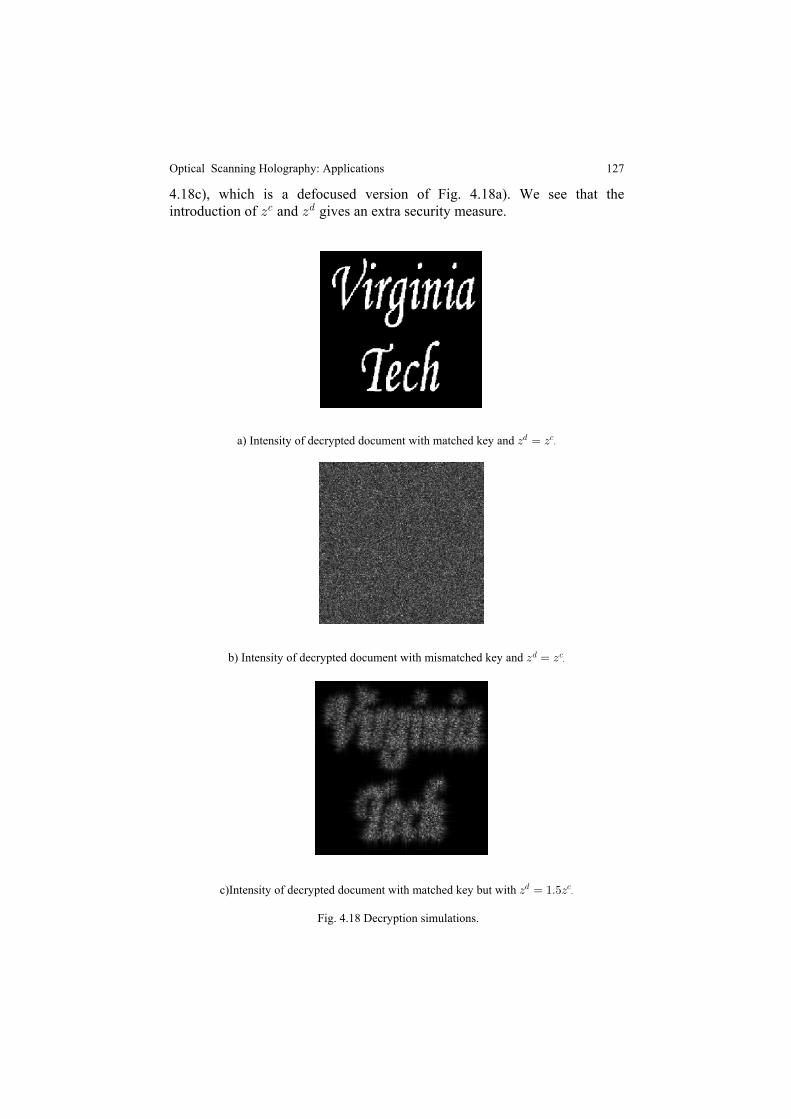
127

4.18c), which is a defocused version of Fig. 4.18a). We see that theintroduction of and gives an extra security measure.D D- .

. -.

b) Intensity of decrypted document with mismatched key and D œ D. -.

c)Intensity of decrypted document with matched key but with D œ "Þ&D. -.

Fig. 4.18 Decryption simulations.


a) Intensity of decrypted document with matched key and D œ D

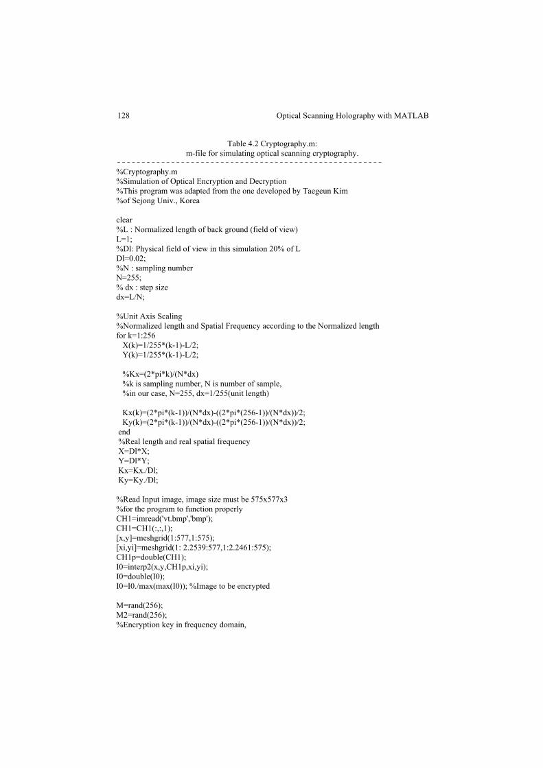
128

Table 4.2 Cryptography.m:m-file for simulating optical scanning cryptography.

------------------------------------------------------%Cryptography.m%Simulation of Optical Encryption and Decryption%This program was adapted from the one developed by Taegeun Kim%of Sejong Univ., Korea

clear%L : Normalized length of back ground (field of view)L=1;%Dl: Physical field of view in this simulation 20% of LDl=0.02;%N : sampling numberN=255;% dx : step sizedx=L/N;

%Unit Axis Scaling%Normalized length and Spatial Frequency according to the Normalized lengthfor k=1:256 X(k)=1/255*(k-1)-L/2; Y(k)=1/255*(k-1)-L/2;

%Kx=(2*pi*k)/(N*dx) %k is sampling number, N is number of sample, %in our case, N=255, dx=1/255(unit length)

Kx(k)=(2*pi*(k-1))/(N*dx)-((2*pi*(256-1))/(N*dx))/2; Ky(k)=(2*pi*(k-1))/(N*dx)-((2*pi*(256-1))/(N*dx))/2; end %Real length and real spatial frequency X=Dl*X; Y=Dl*Y; Kx=Kx./Dl; Ky=Ky./Dl;

%Read Input image, image size must be 575x577x3%for the program to function properlyCH1=imread('vt.bmp','bmp');CH1=CH1(:,:,1);[x,y]=meshgrid(1:577,1:575);[xi,yi]=meshgrid(1: 2.2539:577,1:2.2461:575);CH1p=double(CH1);I0=interp2(x,y,CH1p,xi,yi);I0=double(I0);I0=I0./max(max(I0)); %Image to be encrypted

M=rand(256);M2=rand(256);%Encryption key in frequency domain,


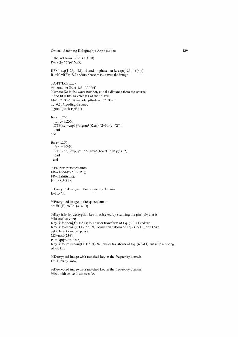
129

%the last term in Eq. (4.3-10)P=exp(-j*2*pi*M2);

RPM=exp(j*2*pi*M); %random phase mask, exp(j*2*pi*r(x,y))R1=I0.*RPM;%Random phase mask times the image

%OTF(kx,ky;zc)%sigma=z/(2Ko)=(z*ld)/(4*pi)%where Ko is the wave number, z is the distance from the source%and ld is the wavelength of the sourceld=0.6*10^-6; % wavelength=ld=0.6*10^-6zc=0.3; %coding distancesigma=(zc*ld)/(4*pi);

for r=1:256, for c=1:256, OTF(r,c)=exp(-j*sigma*(Kx(r).^2+Ky(c).^2)); endend

for r=1:256, for c=1:256, OTF2(r,c)=exp(-j*1.5*sigma*(Kx(r).^2+Ky(c).^2)); end end

%Fourier transformationFR=(1/256)^2*fft2(R1);FR=fftshift(FR);Ho=FR.*OTF;

%Encrypted image in the frequency domainE=Ho.*P;

%Encrypted image in the space domaine=ifft2(E); %Eq. (4.3-10)

%Key info for decryption key is achieved by scanning the pin hole that is%located at z=zcKey_info=conj(OTF.*P); % Fourier transform of Eq. (4.3-11),zd=zcKey_info2=conj(OTF2.*P); % Fourier transform of Eq. (4.3-11), zd=1.5zc%Different random phaseM3=rand(256);P1=exp(j*2*pi*M3);Key_info_mis=conj(OTF.*P1);% Fourier transform of Eq. (4.3-11) but with a wrongphase key

%Decrypted image with matched key in the frequency domainDe=E.*Key_info;

%Decrypted image with matched key in the frequency domain%but with twice distance of zc


130

De2=E.*Key_info2;

%Decrypted image with matched key in the space domainde=ifft2(De); %Eq. (4.3-12)

%Decrypted image with matched key in the space domain%but with zd=1.5 zcde2=ifft2(De2); %Eq. (4.3-12)

%Decrypted image with mis_matched key in the frequency domainDe_mis=E.*Key_info_mis;

%Decrypted image with mis_matched key in the space domainde_mis=ifft2(De_mis);

figure(1)image(X,Y,256*I0);colormap(gray(256));axis squaretitle('image to be encrypted')axis off

figure(2)image(X,Y,255*real(R1));colormap(gray(256));axis squaretitle('Real part of the image multiplied by random phase mask')axis off

figure(3)image(X,Y,255*imag(R1));colormap(gray(256));axis squaretitle('Imaginary part of the image multiplied by random phase mask')axis off

figure(4)image(X,Y,255*abs(e)/max(max(abs(e))))colormap(gray(256))axis squaretitle('Intensity of encrypted image')% absolute value of Eq. (4.3-10)axis off

figure(5)image(X,Y,255*abs(de)/max(max(abs(de))));colormap(gray(256));axis squaretitle('Intensity of decrypted image with matched key with zd=zc')axis off

figure(6)image(X,Y,255*abs(de_mis)/max(max(abs(de_mis))));


131

colormap(gray(256));axis squaretitle('Intensity of decrypted image with mismatched key with zd=zc')axis off

figure(7)image(X,Y,255*abs(de2)/max(max(abs(de2))));colormap(gray(256));axis squaretitle('Intensity of decrypted image with matched key with zd=1.5zc')axis off------------------------------------------------------

References

4.1 Agard, D. A. (1984). Optical sectioning microscopy: cellular architecture in threedimensions,

4.2 Benton, S.A. (1991). Experiments in holographic video, IS-08, 247-Proc. SPIE267.

4.3

4.4 Corle, T. R. and G. S. Kino (1996). Confocal Scanning Optical Microscopy andRelated Imaging Systems, Academic Press, San Diego, CA.

4.5 Enloe, L. H., J.A. Murphy, and C. B. Rubinstein (1966). Hologram transmissionvia television, . 45, 333-335.Bell Syst. Techn. J

4.6 Gabor, D. (1949). Microscopy by reconstructed wavefronts, Proc. Roy. Soc., ser.A, 197, 454-487.

4.7 Hamamatsu Photonics K.K., Japan, and Hamamatsu Corp., Bridgewater, NJ. ImageProcessing and Measuring System (IPMS), Model DVS-3010/SS.

4.8 Hamamatsu Photonics K.K., Japan, and Hamamatsu Corp., Bridgewater, NJ.Product information sheet for EBSLM model X3636.

4.9 Huang, D., E.A. Swanson, C. P. Lin, J.S. Shuman, W.G. Stinson, W. Chang, M.R.Hee, T. Flotte, K. Gregory, C.A. Puliafito, and J. G. Fujimoto (1991). Opticalcoherent tomography, , Vol. 254, 1178-1181.Science

4.10 Indebetouw, G. (2002). Properties of a scanning holographic microscope: improvedresolution, extended depth of focus, and/or optical sectioning, Journal of ModernOptics 49, 1479–1500.

4.11 Indebetouw, G., T. Kim, T.-C. Poon, and B. Schilling (1998). Three-dimensionallocation of fluorescent inhomogeneities in turbid media using scanning heterodyneholography, 23, 135-137.Optics Letters

4.12 Indebetouw, G. and W. Zhong (2006) Scanning holographic microscopy of three-dimensional fluorescent specimens, AJournal of the Optical Society of America 23, 1699-1707.

4.13 Kim, M (2000) Tomographic three-dimensional imaging of a biological specimenusing wave-scanning digital interference holography, 7, 305-310.Optics Express

4.14 Extraction of 3-D location of matched 3-D objectusing power fringe-adjusted filtering and Wigner analysis, 38,Optical Engineering 2176-2183.

4.15 Kirk, R. L. (1984). Electronically generated holography, No.International Patent WO 84/00070.

“”

“ ”

“”

“ ”

“”

“”

“

”“

”

“”

“”

Brown, H. B., S.C. Noble and B.V. Markevitch (1983). Three-dimensional tele-vision system using holographic technique, U.S. Patent # 4,376,950.

Kim, T and T.-C. Poon (1999).


Ann. Rev. Biophys. Bioeng. 13, 191-219.

132

4.16 Lai, S. and M. A. Neifeld (2000). Digital wavefront reconstruction and itsapplications to image encryption, 178, 283-289.Optics Communications

4.17 Lohmann, A.W., W. Stork, and G. Stucke (1986), Optical perfect shuffle, AppliedOptics 25 , 1530-1531.

4.18 Macovski, A. (1971). Considerations of television holography, , 18,Optica Acta31-39.

4.19 Magensen, P.C. and J. Gluckstad (2001). Phase-only optical decryption of a fixedmask, 8, 1226-1235.Applied Optics

4.20 Minsky, M. (1961). Microscopy Apparatus, # 3,013,467.US Patent4.21 Pawley, J. ed. (1995).

Handbook of Biological Confocal Microscopy, 2 ed., Plenum Press.nd

4.22 Poon, T.-C. (2002a). Three-dimensional television using optical scanningholography,” 3, 12-16.Journal of Information Display

4.23 Poon, T.-C. (2002b). inOptical scanning holography: principles and applications,Three-Dimensional Holographic Imaging, C.J. Kuo and M. H. Tsai, ed., John Wiley& Sons, Inc.

4.24 Poon, T.-C. (2005). Three-dimensional optical remote sensing by optical scanningholography, Current Research on Image Processing for 3D information displays,sponsored by SPIE Russia Chapter, V. Petrov, ed., ,Proc. SPIE Vol. 5821, 41-59.

4.25 Poon, T.-C. (2006). Horizontal-parallax-only optical scanning holography, in

Applications, T.-C. Poon ed., Springer, New York, USA.4.26 Poon, T.-C, K. Doh, B. Schilling, M. Wu, K. Shinoda, and Y. Suzuki (1995).

4.27 Poon, T.-C., K. Doh, B. Schilling, K. Shinoda, Y. Suzuki, and M. Wu (1997).Holographic three-dimensional display using an electron-beam-addressed spatial-

light-modulator, 567-571. Optical Review4.28 Poon, T.-C. and T. Kim (1999). Optical image recognition of three-dimensional

objects, 38, 370-381. Applied Optics 4.29 Poon, T.-C., B. D. Schilling, G. Indebetouw, and B. Storrie (2000). Three-

dimensional holographic fluorescence microscopy, # 6,038,041.U.S. Patent4.30 Poon, T.-C., T. Kim, and K. Doh (2003) Optical scanning cryptography for secure

wireless transmission, 42, 6496-6503.Applied Optics4.31 Poon, T.-C., T. Akin, G. Indebetouw and T. Kim (2005). Horizontal-parallax-only

electronic holography 13, 2427-2432., Optics Express4.32 Poon, T.-C. and T. Kim (2006). , WorldEngineering Optics with MATLAB®

Scientific, Singapore.4.33

National Academies Press, Washington, D.C.4.34

plane random phase encoding, 20, 767-769.Optics Letters 4.35 Schilling, B. W. and T.-C. Poon (1995). Real-time pre-processing of holographic

information, 34, 3174-3180. Optical Engineering4.36 Schilling, B. W. (1997). Three-dimensional fluorescence microscopy by optical

scanning holography, Ph.D. dissertation, Virginia Tech.4.37 Schilling, B., T.-C. Poon, G. Indebetouw, B. Storrie, K. Shinoda, and M. Wu

(1997). Three-dimensional holographic fluorescence microscopy, Optics Letters22, 1506-1508.

“”

“ ”

“ ”

“”

“ ”

“

“ ”

“”

“ ”

neering 34, 1338–1344.

“ ”

“”

“”

”

“”

“”

“”

“”

chapter 10 of Digital Holography and Three-Dimensional Display: Principles and

Fundamental limits in confocal microscopy, in chapter 2 of

“Three-dimensional microscopy by optical scanning holography,” Optical Engi-

Radio Frequency Identification Technologies: A Workshop Summary (2004). The

Refregier P. and B. Javidi (1995) “Optical image encryption using input and Fourier


133

4.38 Schilling, B.W. and T.-C. Poon (2004). Multicolor electronic holography and 3-Dimage projection system, # 6760134.U.S. Patent

4.39 Shinoda, K., Y. Suzuki, M. Wu and T.-C. Poon (1991). Optical heterodyne scanningtype holography device, # 5064257.U.S. Patent

4.40

Proc. SPIE, vol. 1212, 174-182.4.41 St. Hilaire, P., S. A. Benton, and M. Lucente (1992). Synthetic aperture

holography: a novel approach to three-dimensional displays, Journal of the OpticalSociety of America A 9, 1969-1977.

4.42 Sun, P and J. -H. Xie (2004).images in scanning holography with a Fresnel-zone-plate coded aperture, AppliedOptics 43, 4214-4218.

4.43 Tajahuerce, E., J. Lancis, B. Javidi, and P. Andres (2001). Optical security andencryption with totally incoherent light, 26, 678-680.Applied Optics

4.44 Wang, B, C.-C. Sun, W.-C. Su, and A. Chiou (2000). Shift-tolerance property of anoptical double-random phase-encoding encryption system, 39,Applied Optics 4788-4793.

4.45 Wilson, T. and C. Sheppard (1984). Theory and Practice of Scanning OpticalMicroscopy , Academic Press.

4.46 Zhang, T. and I. Yamaguchi (1998). Three-dimensional microscopy with phase-shifting digital holography, 23, 1221-1223.Optics Letters

“ ”

“”

“”

“”

“”

“”

Electronic display system for computational holography,J. Underkoffler (1990).St. Hilaire, P., S. A. Benton, M. Lucente, M. Jepsen, J. Kollin, H. Yoshikawa, and

Method for reduction of background artifacts of


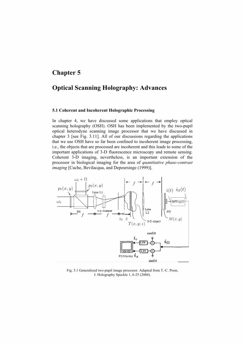
Chapter 5

Optical Scanning Holography: Advances

5.1 Coherent and Incoherent Holographic Processing

In chapter 4, we have discussed some applications that employ opticalscanning holography (OSH). OSH has been implemented by the two-pupiloptical heterodyne scanning image processor that we have discussed inchapter 3 [see Fig. 3.11]. All of our discussions regarding the applicationsthat we use OSH have so far been confined to incoherent image processing,i.e., the objects that are processed are incoherent and this leads to some of theimportant applications of 3-D fluorescence microscopy and remote sensing.Coherent 3-D imaging, nevertheless, is an important extension of theprocessor in biological imaging for the area of quantitative phase-contrastimaging [Cuche, Bevilacqua, and Depeursinge (1999)].

Fig. 5.1 Generalized two-pupil image processor. Adapted from T.-C. Poon,J. Holography Speckle 1, 6-25 (2004).

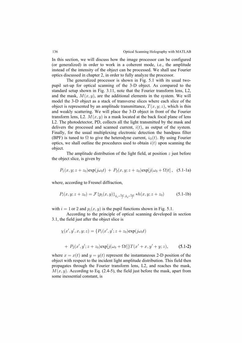
In this section, we will discuss how the image processor can be configured(or generalized) in order to work in a coherent mode, i.e., the amplitudeinstead of the intensity of the object can be processed. We shall use Fourieroptics discussed in chapter 2, in order to fully analyze the processor. The generalized processor is shown in Fig. 5.1 with its usual two-pupil set-up for optical scanning of the 3-D object. As compared to thestandard setup shown in Fig. 3.11, note that the Fourier transform lens, L2,and the mask, , are the additional elements in the system. We willQÐBß CÑmodel the 3-D object as a stack of transverse slices where each slice of theobject is represented by an amplitude transmittance, , which is thinXÐBß Cà DÑand weakly scattering. We will place the 3-D object in front of the Fouriertransform lens, L2. is a mask locateQÐBß CÑ d at the back focal plane of lensL2. The photodetector, PD, collects all the light transmitted by the mask anddelivers the processed and scanned current, , as output of the system.3Ð>ÑFinally, for the usual multiplexing electronic detection the bandpass filter(BPF) is tuned to to give the heterodyne current, . By using FourierH 3 Ð>ÑH

optics, we shall outline the procedures used to obtain upon scanning the3Ð>Ñobject. The amplitude distribution of the light field, just beforeat position Dthe object is given byslice,

, (5.1-1a)T ÐBß Cà D D Ñ Ð4 >Ñ T ÐBß Cà D D Ñ Ò4Ð Ñ>Ó" ! ! # ! !exp exp= = H

where, according to Fresnel diffraction,

(5.1-1b)T ÐBß Cà D D Ñ œ : ÐBß CÑ ‡2ÐBß Cà D D Ñ3 ! !3 5 ß5Y

B C5 B 5 C! !0 0= =

with or and is the pupil functions shown in Fig. 5.1.3 œ " # : ÐBß CÑ3

According to the principle of optical scanning developed in section3.1, t slice he field just after the object is

; =ÐB ß C ß Bß Cà DÑ œ ÖT ÐB ß C à D D Ñ Ð4 >Ñw w w w" ! !exp

, (5.1-2))(5.1-2 T ÐB ß C à D D Ñ Ò4Ð >Ó×X ÐB Bß C Cà DÑ# ! !w w w wexp = H

where and represent the instantaneous 2-D position of theB œ BÐ>Ñ C œ CÐ>Ñobject with respect to the incident light amplitude distribution. This field thenpropagates through the Fourier transform lens, L2, and reaches the mask, QÐBß CÑÞ According to Eq. (2.4-5), the field just before the mask, apart fromsome inessential constant, is


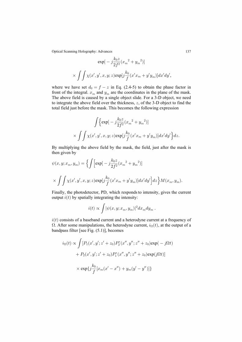
137

expÒ 4 ÐB C ÑÓ5 D

#0!

# 7 7# #

‚ ÐB ß C ß Bß Cà DÑ Ò4 ÐB B C C ÑÓ.B .C5

0( ( ; w w w w w w!

7 7exp ,

where we have set in Eq. (2.4-5) to obtain the phase factor in. œ 0 D!

front of the integral. and are the coordinatesB C7 7 in the plane of the mask.The above field is caused by a single object slide. For a 3-D object, we needto integrate the above field over the thickness, , of the 3-D object to find theDtotal field just before the mask. This becomes the following expression

( šexpÒ 4 ÐB C ÑÓ5 D

#0!

# 7 7# #

‚ ÐB ß C ß Bß Cà DÑ Ò4 ÐB B C C ÑÓ.B .C .D5

0( ( ›; w w w w w w!

7 7exp .

By multiplying the above field by the mask, the field, just after the mask isthen given by

<ÐBß Cà B ß C Ñ œ Ò 4 ÐB C ÑÓ5 D

#07 7 7 7!

## #š ’( exp

‚ ÐB ß C ß Bß Cà DÑ Ò4 ÐB B C C ÑÓ.B .C .D QÐB ß C Ñ5

0( ( “ ›; w w w w w w!

7 7 7 7exp .

Finally, the photodetector, PD, which responds to intensity, gives currentthe output by spatially integrating the intensity:3Ð>Ñ

3Ð>Ñ º l ÐBß Cà B ß C Ñl .B .C( < 7 7 7 7# .

3Ð>Ñ consists of a baseband current and a heterodyne current at a frequency ofH. After some manipulations, the heterodyne current, , at the output of a3 Ð>ÑH

bandpass filter [see Fig. (5.1)], becomes

3 Ð>Ñ º T B ß C à D D T B ß C à D D 4 >H ( c a b a b a b" ! !w w w ‡ ww ww ww

# exp H

a b a b a b T B ß C à D D T B ß C à D D 4 > Ó# ! !w w w ‡ ww ww ww

" exp H

‚ Ö4 ÒB ÐB B Ñ C ÐC C ÑÓ×5

0exp !

7 7w ww w ww


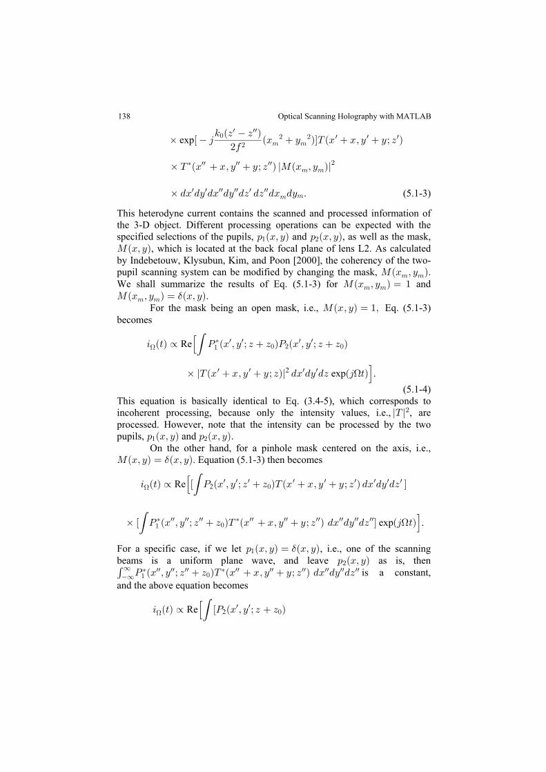
138

‚ Ò 4 ÐB C ÑÓX ÐB Bß C Cà D Ñ5 ÐD D Ñ

#0exp !

w ww

# 7 7# # w w w

‚ X ÐB Bß C Cà D Ñ QÐB ß C Ñ‡ ww ww ww7 7

#k k‚ .B .C .B .C .D .D .B .Cw w ww ww w ww

7 7. (5.1-3)

This heterodyne current contains the scanned and processed information ofthe 3-D object. Different processing operations can be expected with thespecified selections of the pupils, and , as well as the mask,: ÐBß CÑ : ÐBß CÑ1 #

QÐBß CÑ, which is located at the back focal plane of lens L2. As calculatedby Indebetouw, Klysubun, Kim, and Poon [2000], the coherency of the two-pupil scanning system can be modified by changing the mask, .QÐB ß C Ñ7 7

We shall summarize the results of Eq. (5.1-3) for andQÐB ß C Ñ œ "7 7

QÐB ß C Ñ œ ÐBß CÑ7 7 $ . For the mask being an open mask, i.e., Eq. (5.1-3)QÐBß CÑ œ "ßbecomes

3 Ð>Ñ ºH Re’( T ÐB ß C à D D ÑT ÐB ß C à D D Ñ‡ w w w w" ! # !

‚ l ÐB Bß C Cà DÑl .B .C .D Ð4 >ÑX w w w w2 exp H “.(5.1-4)

This equation is basically identical to Eq. (3.4-5), which corresponds toincoherent processing, because only the intensity values, i.e., , arelX l#

processed. However, note that the intensity can be processed by the twopupils, : ÐBß CÑ : ÐBß CÑ1 and .#

On the other hand, for a pinhole mask centered on the axis, i.e.,QÐBß CÑ œ ÐBß CÑ$ . Equation (5.1-3) then becomes

3 Ð>Ñ º Ò T ÐB ß C à D D ÑX ÐB Bß C Cà D Ñ .B .C .D ÓH Re’ ( 2w w w w w w w w w

!

‚ Ò T ÐB ß C à D D ÑX ÐB Bß C Cà D Ñ .B .C .D Ó Ð4 >Ñ( “‡ ww ww ww ‡ ww ww ww ww ww ww" ! exp H .

For a specific case, if we let , i.e., one of the scanning: ÐBß CÑ œ ÐBß CÑ1 $beams is a uniform plane wave, and leave as is, then: ÐBß CÑ#'__ ‡ ww ww ww ‡ ww ww ww ww ww ww

" !T ÐB ß C à D D ÑX ÐB Bß C Cà D Ñ .B .C .D is a constant,and the above equation becomes

3 Ð>Ñ ºH Re’( ÒT ÐB ß C à D D Ñ2w w

!


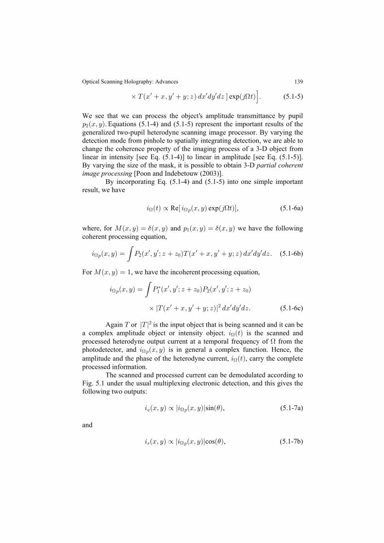
139

‚ X Ð4 >ÑÐB Bß C Cà DÑ .B .C .D Ów w w w exp H “. (5.1-5)

We see that we can process the object s amplitude transmittance by pupil: ÐBß CÑ# . Equations (5.1-4) and (5.1-5) represent the important results of thegeneralized two-pupil heterodyne scanning image processor. By varying thedetection mode from pinhole to spatially integrating detection, we are able tochange the coherence property of the imaging process of a 3-D object fromlinear in intensity [see Eq. (5.1-4)] to linear in amplitude [see Eq. (5.1-5)].By varying the size of the mask, it is possible to obtain 3-D partial coherentimage processing [Poon and Indebetouw (2003)]. By incorporating Eq. (5.1-4) and (5.1-5) into one simple importantresult, we have

3 Ð>Ñ º 3 ÐBß CÑ Ð4 >ÑH HRe , (5.1-6a)c d: exp H

where, the followingfor and we haveQÐBß CÑ œ ÐBß CÑ : ÐBß CÑ œ ÐBß CÑ$ $1coherent processing equation,

. (5.1-6b)3 ÐBß CÑ œ T ÐB ß C à D D Ñ ÐB Bß C Cà DÑ .B .C .DH:w w w w w w

!( 2 X

F , we have the incoherent processing equation,or QÐBß CÑ œ "

3 ÐBß CÑ œ T ÐB ß C à D D ÑT ÐB ß C à D D ÑH:‡ w w w w" ! # !(

. (5.1-6c)‚ l ÐB Bß C Cà DÑl .B .C .DX w w # w w

Again or is the input object that is being scanned and it can beX lX l#

a complex amplitude object or intensity object. 3 Ð>ÑH is the scanned andprocessed heterodyne output current at a temporal frequency of from theHphotodetector, and is in general a complex function. Hence, the3 ÐBß CÑH:

amplitude and the phase of the heterodyne current, , carry the complete3 Ð>ÑH

processed information. The scanned and processed current can be demodulated according toFig. 5.1 under the usual multiplexing electronic detection, and this gives thefollowing two outputs:

sin , (5.1-7a)3 ÐBß CÑ º l3 ÐBß CÑl Ð Ñc H: )

and

cos , (5.1-7b)3 ÐBß CÑ º l3 ÐBß CÑl Ð Ñ= :H )

’


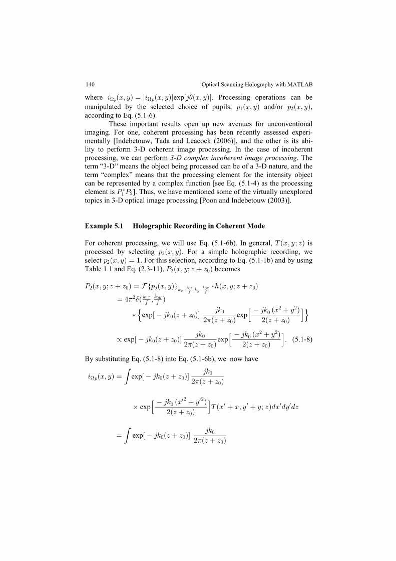
140

where exp . Processing operations can be3 ÐBß CÑ œ l3 ÐBß CÑl Ò4 ÐBß CÑÓH H: : )

manipulated by the selected choice of pupils, : ÐBß CÑ : ÐBß CÑ1 2 and/or ,according to Eq. (5.1-6). These important results open up new avenues for unconventional

processing, we can perform . The3-D complex incoherent image processingterm 3-D means the object being processed can be of a 3-D nature, and theterm complex means that the processing element for the intensity objectcan be represented by a complex function [see Eq. (5.1-4) as the processingelement is . Thus, we have mentioned some of the virtually unexploredT T‡" #]topics in 3-D optical image processing [Poon and Indebetouw (2003)].

Example 5.1 Holographic Recording in Coherent Mode

For coherent processing, we will use Eq. (5.1-6b). In general, XÐBß Cà DÑ isprocessed by selecting : ÐBß CÑ2 . For a simple holographic recording, weselect . For this selection, according to Eq. (5.1-1b) and by using: ÐBß CÑ œ "2Table 1.1 and Eq. (2.3-11), becomesT ÐBß Cà D D Ñ# !

T ÐBß Cà D D Ñ œ : ÐBß CÑ ‡2ÐBß Cà D D Ñ# ! !# 5 ß5Y

B C5 B 5 C! !0 0= =

œ %1 $# Ð Ñ5 B0 0

5 C! !,

‡ D DD D D D

š ›exp expÒ 45 Ð ÑÓ45

# Ð Ñ Ð Ñ!

!!

! !1’ 45 ÐB C Ñ

#!

# # “ exp exp (5.1-8)º Ò 45 Ð ÑÓ

45

# Ð Ñ Ð Ñ!

!D D

D D D D!

! !1’ 45 ÐB C Ñ

#!

# # “.

By substituting Eq. (5.1-8) into Eq. (5.1-6b), we now have

3 ÐBß CÑ œH: ( expÒ 45 Ð ÑÓ45

# Ð Ñ!

!D D

D D!

!1

; ‚ ÐB Bß C C .B .C .Dexp’ 45 ÐB C Ñ

#X!

w w# #

Ð ÑDÑ

D D!“ w w w w

œ ( expÒ 45 Ð ÑÓ45

# Ð Ñ!

!D D

D D!

!1

imaging. For one, coherent processing has been recently assessed experi-mentally [Indebetouw, Tada and Leacock (2006)], and the other is its abi-lity to perform 3-D coherent image processing. In the case of incoherent

“ ”“ ”


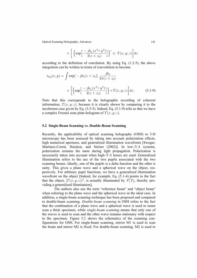
141

‚ ÐBß Cà DÑ .D” •šexp’ 45 ÐB C Ñ

#Œ!

# # ‡+ Ð ÑD D

X!

“›

according to the definition of correlation. By using Eq. (1.2-5), the aboveintegration can be written in terms of convolution to become

3 ÐBß CÑ œH: ( expÒ 45 Ð ÑÓ45

# Ð Ñ!

!D D

D D!

!1

. (5.1-9)‚ ÐBß Cà DÑ .D” •šexp’ 45 ÐB C Ñ

#‡ X!

# #+ Ð ÑD D!

“›Note that this corresponds to the holographic recording of coherentinformation, , because it is clearly shown by comparing it to theXÐBß Cà DÑincoherent case given by Eq. (3.5-5). Indeed, Eq. (5.1-9) tells us that we havea complex Fresnel zone plate hologram of .XÐBß Cà DÑ

5.2 Single-Beam Scanning vs. Double-Beam Scanning

Recently, the applicability of optical scanning holography (OSH) to 3-Dmicroscopy has been assessed by taking into account polarization effects,high numerical apertures, and generalized illumination wavefronts [Swoger,Martinez-Corral, Huisken, and Stelzer (2002)]. In low- systems,REpolarization remains the same during light propagation. Polarization isnecessarily taken into account when high- lenses are used. GeneralizedREillumination refers to the use of the two pupils associated with the twoscanning beams. Ideally, one of the pupils is a delta function and the other is

that the object, lX ÐBß C DÑl T; , is actually illuminated by #" #*

The authors also use the term reference beam and object beamwhen referring to the plane wave and the spherical wave in the ideal case. Inaddition, a single-beam scanning technique has been proposed and comparedto double-beam scanning. in OSH refers to the factDouble-beam scanningthat the combination of a plane wave and a spherical wave is used to rasterscan a thick specimen, while means that only one ofsingle-beam scanning the waves is used to scan and the other wave remains stationary with respect

the beam and mirror M2 is fixed. For double-beam scanning, M2 is used to

“ ” “ ”

unity. This gives a plane wave and a spherical wave on the object, res-pectively. For arbitrary pupil functions, we have a generalized illuminationwavefront on the object [Indeed, for example, Eq. (5.1-4) points to the fact

T , thereby pro-viding a generalized illumination].

to the specimen. Figure 5.2 shows the schematics of the scanning con-figurations for OSH. For single-beam scanning, mirror M1 is used to scan


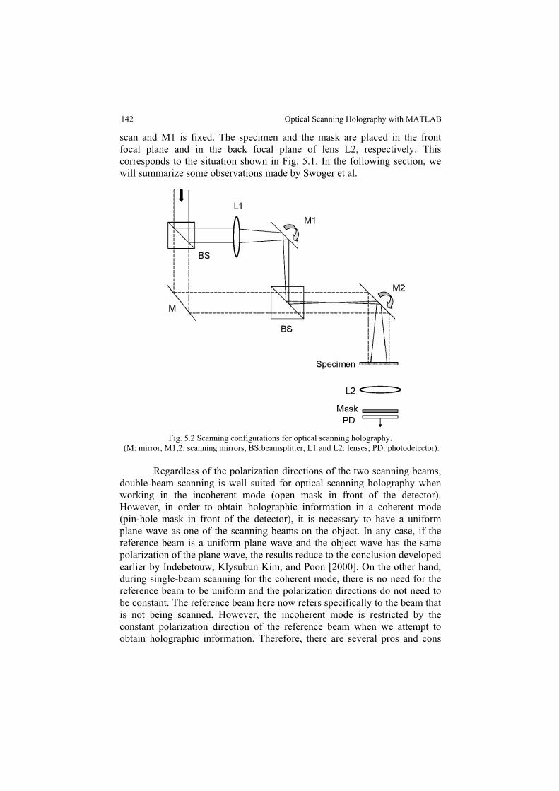
142

scan and M1 is fixed. The specimen and the mask are placed in the frontfocal plane and in the back focal plane of lens L2, respectively. Thiscorresponds to the situation shown in Fig. 5.1. In the following section, wewill summarize some observations made by Swoger et al.

Fig. 5.2 Scanning configurations for optical scanning holography. (M: mirror, M1,2: scanning mirrors, BS:beamsplitter, L1 and L2: lenses; PD: photodetector).

Regardless of the polarization directions of the two scanning beams,double-beam scanning is well suited for optical scanning holography whenworking in the incoherent mode (open mask in front of the detector).However, in order to obtain holographic information in a coherent mode(pin-hole mask in front of the detector), it is necessary to have a uniformplane wave as one of the scanning beams on the object. In any case, if thereference beam is a uniform plane wave and the object wave has the samepolarization of the plane wave, the results reduce to the conclusion developedearlier by Indebetouw, Klysubun Kim, and Poon [2000]. On the other hand,during single-beam scanning for the coherent mode, there is no need for thereference beam to be uniform and the polarization directions do not need tobe constant. The reference beam here now refers specifically to the beam thatis not being scanned. However, the incoherent mode is restricted by theconstant polarization direction of the reference beam when we attempt toobtain holographic information. Therefore, there are several pros and cons


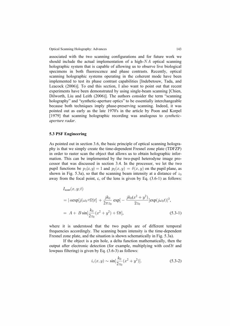
143

associated with the two scanning configurations and for future work weshould include the actual implementation of a high- optical scanningREholographic system that is capable of allowing us to observe live biologicalspecimens in both fluorescence and phase contrasts. Recently, opticalscanning holographic systems operating in the coherent mode have beenimplemented to test its phase contrast capabilities [Indebetouw, Tada, andLeacock (2006)]. To end this section, I also want to point out that recentexperiments have been demonstrated by using single-beam scanning [Chien,Dilworth, Liu and Leith (2006)]. The authors consider the term scanningholography and synthetic-aperture optics to be essentially interchangeablebecause both techniques imply phase-preserving scanning. Indeed, it waspointed out as early as the late 1970 s in the article by Poon and Korpel[1979] that scanning holographic recording was analogous to synthetic-aperture radar.

5.3 PSF Engineering

" and : ÐBß CÑ œ ÐBß CÑ# $

!

M ÐBß Cà >Ñscan

œ l + Ò4Ð Ñ>Ó Ò Ó Ð4 >Ñl45 45 B C Ñ

D #Dexp + exp exp ,

2(

= H =1

! !! !

! !

#2 2

, (5.3-1)2


Dsin !

!

2 2 H

where it is understood that the two pupils are of different temporalfrequencies accordingly. The scanning beam intensity is the time-dependentFresnel zone plate, and the situation is shown schematically in Fig. 5.3a). If the object is a pin hole, a delta function mathematically, then theoutput after electronic detection (for example, multiplying with cos andH>lowpass filtering) is given by Eq. (3.6-3) as follows:


D-

!

!sin

2. (5.3-2)2 2

“” “ ”

’

As pointed out in section 3.6, the basic principle of optical scanning hologra-phy is that we simply create the time-dependent Fresnel zone plate (TDFZP)in order to raster scan the object that allows us to obtain holographic infor-mation. This can be implemented by the two-pupil heterodyne image pro-cessor that was discussed in section 3.4. In the processor, we let the twopupil functions be : ÐBß CÑ œ "shown in Fig. 5.3a), so that the scanning beam intensity at a distance of

on the pupil plane, asD

away from the focal point, c, of the lens is given by Eq. (3.6-1) as follows:


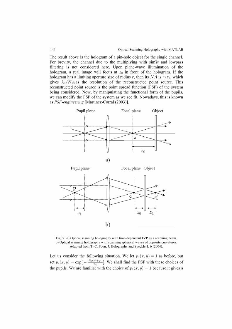
144

The result above is the hologram of a pin-hole object for the single channel.For brevity, the channel due to the multiplying with sin and lowpassH>filtering is not considered here. Upon plane-wave illumination of thehologram, a real image will focus at in front of the hologram. If theD!hologram has a limiting aperture size of radius , then its is , which< RE <ÎD0gives as the resolution of the reconstructed point source. This-0ÎREreconstructed point source is the point spread function (PSF) of the systembeing considered. Now, by manipulating the functional form of the pupils,we can modify the PSF of the system as we see fit. Nowadays, this is knownas [Martinez-Corral (2003)].PSF-engineering

Fig. 5.3a) Optical scanning holography with time-dependent FZP as a scanning beam.b) Optical scanning holography with scanning spherical waves of opposite curvatures.

Adapted from T.-C. Poon, J. Holography and Speckle 1, 6 (2004).

"

set exp . We shall find the PSF with these choices of: ÐBß CÑ œ Ò Ó#45 B C Ñ

#D!

3

( 2 2

the pupils. We are familiar with the choice of because it gives a: ÐBß CÑ œ ""

Let us consider the following situation. We let : ÐBß CÑ œ " as before, but


145

spherical wave on the object at a distance away from the focal plane of theD!

lens, which corresponds to the term exp exp in Eq.45D #D

45 B C Ñ!

!

! !

!

2(

1Ò Ó Ð4 >Ñ

2 2=

(5.3-1). The situation is shown in Fig. 5.3b). Let us find what is in Eq.+(5.3-1) for the choice of given above. Note that is now a: ÐBß CÑ +ÐBß CÑ#

function of and . Through the Fourier transformation of the lens [see Eq.B C(2.4-6)] and Fresnel diffraction at a distance of [see Eq. (2.3-12)], we canD!write the field distribution due to on the object as: ÐBß CÑ#

(5.3-3)+ÐBß CÑ œ : ÐBß CÑ DYBCÖ × ‡ 2ÐBß Cà Ñ# !º5Cœ5 CÎ0!

5 œ5 BÎ0B !

œ Ò Ó D45 ÐB C Ñ

#D expYBC˜ ™º!

3!

2 2

5 œ5 CÎ0C !

5 œ5 BÎ0B !

‡ 2ÐBß Cà Ñ,

where is the focal length of the lens. The above Fourier transformation can0be found by using Table 1.1 on page 2. We then perform the convolution andthe result, apart from some constant, is given as follows:

+ÐBß CÑ œ Ò Ó45 45 ÐB C Ñ

D #D! !

" "2exp . (5.3-4)

1

2 2

w

"

"

3

" " "

0 D 0 D D 0 œ

3 ! " . (5.3-5)

Therefore, we can design with a different radius of curvature.: ÐBß CÑ#

For the choices of and , Eq. (5.3-5) will beD œ #0 D œ D œ 0Î%3 ! "

satisfied. Since , we will have spherical waves of opposite curvaturesD œ D! "

illuminating the specimen. Hence, with Eq. (5.3-4) and , the scanningD œ D! "

beam intensity becomes

M ÐBß Cà >Ñscan

º l Ò Ó Ò4Ð Ñ>Ó Ò Ó Ð4 >Ñl45 ÐB C Ñ 45 ÐB C Ñ

#D #Dexp exp exp exp! !

! !! !

#2 2 2 2

= H =

Note that +ÐBß CÑ can either be converging wavefronts or divergent wave-fronts on the specimen and this is dependent on the location of the focusedpoint, p. In Fig. 5.3b), we show that point c is the image point of the focusedpoint, p, and hence the radius of curvature, D , is positive in the situation

Example 2.4 on spherical wave]. The value of D can be designed accordinglyby properly locating point p or the distance, D , under the imaging conditionso that

because we have converging wavefronts illuminating the specimen [see


146

, (5.3-6)2


ÐD Î#Ñw w !

!sin 2 2 H

where and are some constants. The above scanning beam givesE Fw w


D-

!

!sin 2 2 (5.3-7)

as our new hologram for the selected pupils. Upon real image reconstructionof the hologram given by Eq. (5.3-7), we see that the image is formed at adistance of . For the same limiting aperture size of the hologram, ,D Î# <!

similar to the standard optical scanning setup, its now becomesRE<ÎÐD Î#Ñ ÎÐ#REÑ0 0. This gives as the resolution of the reconstructed point-source, which is our new PSF. The result means that for the same hologramaperture size, it is possible to synthesize the point-spread function in opticalscanning holography in order to obtain holographic reconstructions with atransverse resolution exceeding the Rayleigh limit of the aperture up to afactor of 2, at least in the limit of low . Indeed, this has been investigatedREby Indebetouw (2002) and was recently confirmed by optical experiments[Indebetouw, Maghnouji, and Foster (2005)]. Other pupils examined so farinclude , which have been used to achieve optical sectioning,axiconshowever, thus far only simulations have been provided [Indebetouw, Zhong,and Chamberlin-Long (2006)]. In general, arbitrary complex amplitude distributions of the pupilscan be synthesized by using masks, refractive or diffractive optical elements(DOEs), or spatial light modulators which allow dynamic changes. For: ÐBß CÑ œ Ò #

45 B C Ñ#Dexp !

!

( 2 2

3

plane as shown in Fig. 5.3b). In general, I want to point out that the two-pupil method offers a broad range of possibilities when synthesizing

applications is [Indebetouw, Tada, Rosen and Brookersuper-resolution(2007)].

References

5.1 Chien, W.-C., D. S. Dilworth, E. Liu, and E. N. Leith (2006). Synthetic-aperturechirp confocal imaging, 45, 501-510.Applied Optics

5.2 Cuche, E., F. Bevilacqua, and C. Depeursinge (1999).quantitative phase-contrast imaging, 24, 291-293.Optics Letters

Ó shown in this example, we can simply imple-ment it by placing a point source at a distance, D , in front of the pupil

“”

”

unconventional PSFs for potential novel applications. One of the new

“Digital holography for


147

5.3 Indebetouw, G. (2002). Properties of a scanning holographic microscope: improvedresolution, extended depth of focus, and/or optical sectioning, Journal of ModernOptics 49, 1479-1500.

5.4 Indebetouw, G., P. Klysubun, T. Kim, and T.-C. Poon (2000). Imaging propertiesof scanning holographic microscopy, Journal of the Optical Society of America A17, 380-390.

5.5 Indebetouw, G., A. El Maghnouji, and R. Foster (2005). Scanning holographicmicroscopy with transverse resolution exceeding the Rayleigh limit and extendeddepth of focus, 22, 829-898.Journal of the Optical Society of America A

5.6 Indebetouw, G., Y. Tada and J. Leacock (2006). Quantitative phase imaging withscanning holographic microscopy: an experimental assessment, available athttp://www.biomedical-engineering-online.com/content/5/1/63.

5.7 Indebetouw, G., W. Zhong, and D. Chamberlin-Long (2006). Point-spread functionsynthesis in scanning holographic microscopy, Journal of the Optical Society ofAmerica A 23, 1708-1717.

5.8 Indebetouw, J., Y. Tada, J. Rosen, and G. Brooker (2007). Scanning holographicmicroscopy with resolution exceeding the Rayleigh limit of the objective bysuperposition of off-axis holograms, , to appear.Applied Optics

5.9 Martinez-Corral, M. (2003). Point spread function engineering in confocalscanning microscopy, , Vol. 5182, 112-122.Proceedings of SPIE

5.10 Poon, T.-C. and A. Korpel (1979). Optical transfer function of an acousto-opticheterodyning image processor, 4, 317-319.Optics Letters

5.11 Poon, T.-C. (2004). Recent progress in optical scanning holography , Journal ofHolography and Speckle 1, 6-25.

5.12 Poon, T.-C. and G. Indebetouw (2003). Three-dimensional point spread functionsof an optical heterodyne scanning image processor, 42, 1485-1492.Applied Optics

5.13 Swoger, J., M. Martínez-Corral, J. Huisken, and E. H. K. Stelzer (2002). Opticalscanning holography as a technique for high-resolution three-dimensional biologicalmicroscopy, 19, 1910-1918.Journal of the Optical Society of America A

“

”

“”

“ ”

“”

“”

“

”

“”

“”

“

”

“”

“”


Index

A acousto-optic frequency shifter 72 acousto-optic modulator 72 angular frequency 25 aperture 29 axicon 146 B bipolar PSF 46,49 bitmap 7 Bragg angle 73 C carrier 30 coding process 55 coherent point spread function 44 coherent transfer function 45 complex amplitude 30 conservation of energy 73 conservation of momentum 73 constitution relations 22 continuity equation 22 convolution 14, 16 correlation 14, 16 auto- 17

cross- 17 current baseband 70 heterodyne 70 D decoding process 55 decryption 121 depth of field 100 depth of focus 97 detection electronic multiplexing 70 lock-in 70 optical coherent 70 optical direct 67 optical incoherent 67 diffracting screen 29 display 3-D 106 distance coding 120 decoding 122 E electric field 22 encoding

double-random phase 124

encryption 121 on-the-fly 118 F filtering bandpass 48 lowpass 47 spatial 45 Fourier optics

spatial frequency transferfunction in 34

spatial impulse response in 34 Fourier plane 43 frequency transfer function 13 Fourier transform 1 Fresnel diffraction 34 Fresnel diffraction formula 34 Fresnel zone plate (FZP) 49, 52 time-dependent 92, 102 function Gaussian 2 separabale 3

transfer 13 G Gaussian beam 40 Gaussian function 2 H Helmholtz equation 30 heterodyning 69 hologram 51 complex Fresnel zone plate 85

cosine-FZP 83 off-axis 59 sine-FZP 83 twin-image-free 83 hologram scaling 110, 113

holographic recording 51 holography 49 carrier-frequency 60 CO2 scanning 84 digital 60 electronic 62 HPO-optical scanning 117 phase-shifting 85 scanning 65, 81 off-axis 56 X-ray scanning 84 homodyning 94 I ideal lens 40 image intensity 45 image processing 3-D complex incoherent 140 bipolar incoherent 48 coherent 43 complex incoherent 78 incoherent 44 impulse response 11 initial condition 29 in-phase component 71 integral convolution 11 correlation 16 invariance 10 issue

spatial frequency resolution115

spatial resolution 116 data transmission 117 K key

decryption 122 encryption 121

150

delta 2, 8

rect 2, 3

sinc 2, 4

optical scanning 65, 83, 87, 92


lateral resolution 97 linearity 10 liquid crystal television 61 lock-in detection 70 M magnetic field 22 magnification lateral 113 longitudinal 113 holographic 112 Maxwell’s equations 21 medium homogeneous 22 isotropic 22 linear 22 microscopy fluorescence 101 optical sectioning 99 scanning confocal 99 scanning holographic 97 mixing 70 modulator acousto-optic 72

electron-beam-addressed spatial light 107

N numerical aperture 98 Nyquist sampling 116 O optical coherent detection 70 optical coherent tomography (OCT) 101 optical direct detection 67 optical heterodyning 65, 69 optical incoherent detection 67 optical pattern recognition 17 optical scanning 65

optical scanning holography 65, 97, 117 HPO- 117

optical transfer function(OTF) 46, 78

P parallax 49 paraxial approximation 33 pattern recognition 17 phase 26 phase curvature 42 phase grating 73 phasor 30 phonon 73 photo-bleaching 101 photon 73 planar wavefront 27 Planck’s constant 73 Pockels effect 108 point spread function (PSF) 13 bipolar 46

coherent 44 complex 49 intensity 46

principle of conservation of charge 22 processing coherent holographic 136 Fourier-plane 43 incoherent holographic 136 propagation constant 26 propagation vector 26 PSF-engineering 143 pupil function 45

Q quadrature component 71 quantitative phase-contrast

imaging 133

151

L optical scanning cryptography 117

Index

radio frequency identification (RFID) 118 radius of curvature 35 real image 56, 60 reconstruction 55 recording 55 recording angle 58 S sampling property 9 scalar diffraction theory 29 scalar wave equation 25 scanning single-beam 141 double-beam scanning 141 separable function 3 solution planar wave 25 spherical wave 27 source 22 spatial carrier 60 spatial filter 44 spatial frequency response 13 spatial frequency transfer function in Fourier optics 34 spatial frequency transfer function of propagation 31 spatial impulse response in Fourier optics 34 spatial impulse response 13 spatial impulse response of propagation 33 spatial light modulator (SLM) 61 electron-beam addressed 107 spherical wavefront 28 square aperture 36 superposition 10

super-resolution 146 synthetic-aperture radar 143 system coherent optical 45

incoherent optical 45 linear 10 linear space-invariant 12 time-invariant 11 two-pupil 75 T TV holographic 106 twin image 57 twin-image problem 58 two-pupil system 75 U uncertainty relationship 99 upshifted interaction 74 V vector wave equation 23 homogeneous 24 viewing angle 115 virtual image 57, 60 W Wave divering spherical 35 object 51 plane 26 reconstruction 55, 59 reference 51 spherical 28, 52 wavelength scaling 114 Z

R


zero-order beam 56, 59

Author

Ting-Chung Poon Bradley Department of Electrical and Computer Engineering Virginia Tech Blacksburg, Virginia, USA 24061 e-mail: [email protected] Dr. Ting-Chung Poon received his physics and engineering degrees from the

Bradley Department of Electrical and Computer Engineering. His currentUniversity of Iowa, Iowa City. He is a professor at Virginia Tech in the

research interests include acousto-optics, hybrid (optical/electronic/digital)3-D image processing; optical scanning holography and its applications in3-D cryptography, 3-D display, 3-D microscopy, 3-D optical remote sensing,and 3-D pattern recognition. Dr. Poon is the co-author of the textbooks Engineering Optics with MATLAB® (World Scientific 2006), Contemporary Optical Image Processing with MATLAB® (Elsevier 2001), and Principles of Applied Optics (McGraw-Hill 1991). He is also editor of the book Digital Holography and Three-Dimensional Display (Springer 2006) and has served as a panelist for the National Institutes of Health and the National Science Foundation, and as guest editor of, among other journals, International Journal of Optoelectronics and Optical Engineering. Dr. Poon currently serves as a topical/associate editor for Applied Optics and the International Journal of Optomechatronics. He is also on the editorial board of Optics and Laser Technology and the Journal of Holography and Speckle. Dr. Poon is a fellow of the OSA and SPIE and is a senior member of the IEEE.