Modelling fast transient flows and

morphological evolution in rivers

Sandra Soares-Frazão

Civil Engineering

Université catholique de Louvain

1

Contents

• Mathematical models

• Open questions

– 1D approach

– Steep slopes

– Sediment transport

• Application to breaching

2

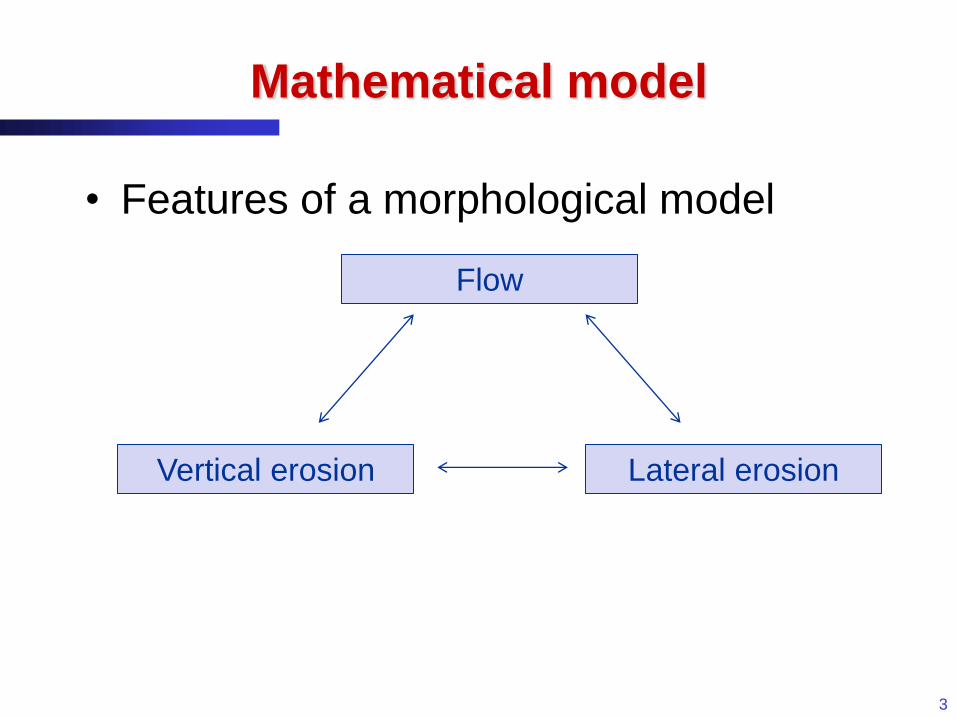
Mathematical model

• Features of a morphological model

3

Flow

Vertical erosion Lateral erosion

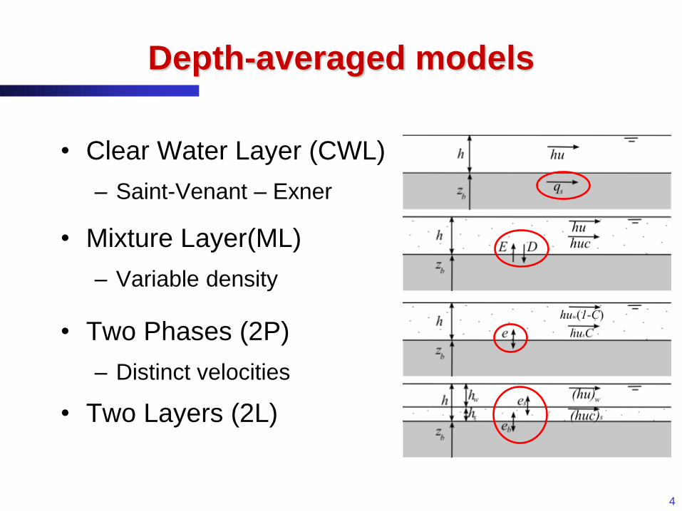
Depth-averaged models

• Clear Water Layer (CWL)

– Saint-Venant – Exner

• Mixture Layer(ML)

– Variable density

• Two Phases (2P)

– Distinct velocities

• Two Layers (2L)

4

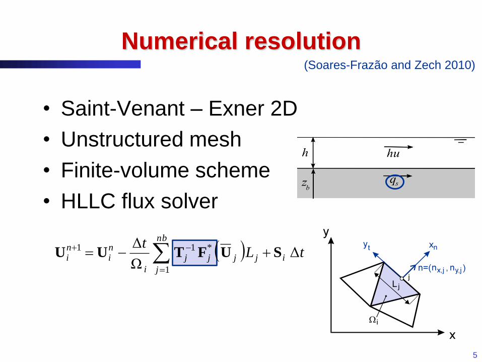
Numerical resolution

• Saint-Venant – Exner 2D

• Unstructured mesh

• Finite-volume scheme

• HLLC flux solver

5

(Soares-Frazão and Zech 2010)

tLt

i

nb

j

jj*jj

i

ni

ni Δ

Ω

Δ

1

11SUFTUU

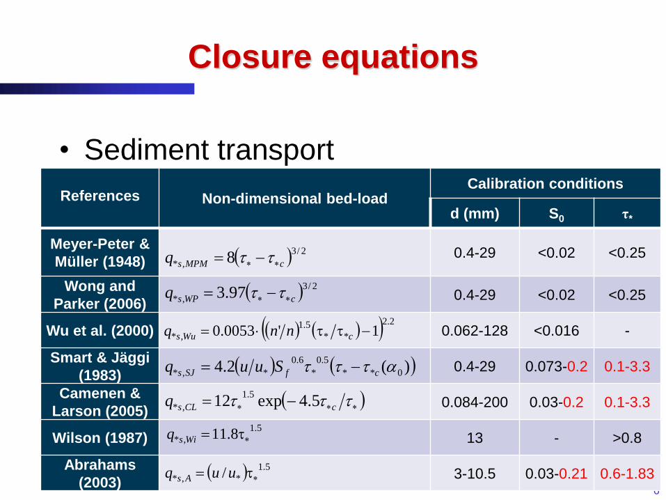
Closure equations

• Sediment transport

• Formules empiriques, calibrées dans

des conditions limitées

6

References Non-dimensional bed-load Calibration conditions

d (mm) S0 τ*

Meyer-Peter &

Müller (1948) 0.4-29 <0.02 <0.25

Wong and

Parker (2006) 0.4-29 <0.02 <0.25

Wu et al. (2000) 0.062-128 <0.016 -

Smart & Jäggi

(1983) 0.4-29 0.073-0.2 0.1-3.3

Camenen &

Larson (2005) 0.084-200 0.03-0.2 0.1-3.3

Wilson (1987) 13 - >0.8

Abrahams

(2003) 3-10.5 0.03-0.21 0.6-1.83

2/3

,* 8 cMPMsq

2/3

,* 97.3 cWPsq

)(2.4 0**

5.0

*

6.0

*,* cfSJs Suuq

5.1

*,* / uuq As

cCLsq 5.4exp125.1

,*

2.2

**

5.1

,* 1'0053.0 cWus nnq

5.1

,* 8.11 Wisq

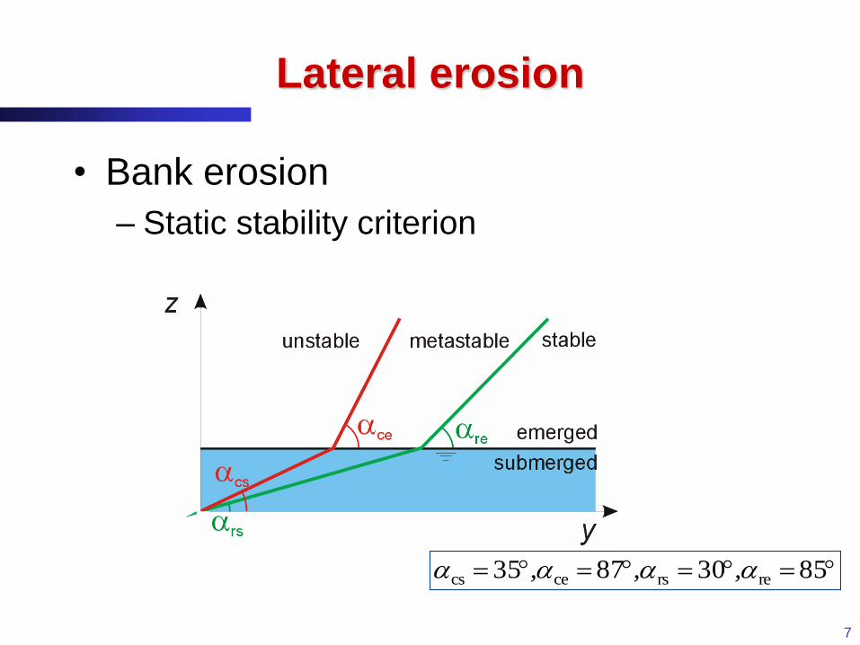
Lateral erosion

• Bank erosion

– Static stability criterion

7

85308735 rerscecs ,,,

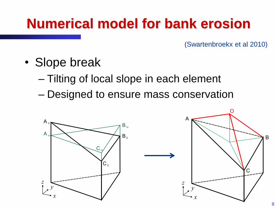
Numerical model for bank erosion

• Slope break

– Tilting of local slope in each element

– Designed to ensure mass conservation

8

(Swartenbroekx et al 2010)

Contents

• Mathematical models

• Open questions

– 1D approach

– Sediment transport: bed shear stress

– Steep slopes

• Application to breaching

9

Open questions

• 1D approaches

– Efficiency?

– Accuracy?

– Extension to morphological evolution?

10

11

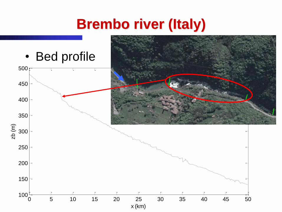
Brembo river (Italy)

• Bed profile

0 5 10 15 20 25 30 35 40 45 50100

150

200

250

300

350

400

450

500

x (km)

zb

(m

)

12

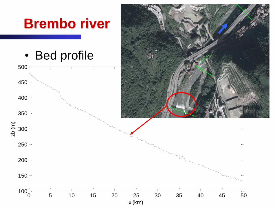
Brembo river

• Bed profile

0 5 10 15 20 25 30 35 40 45 50100

150

200

250

300

350

400

450

500

x (km)

zb

(m

)

13

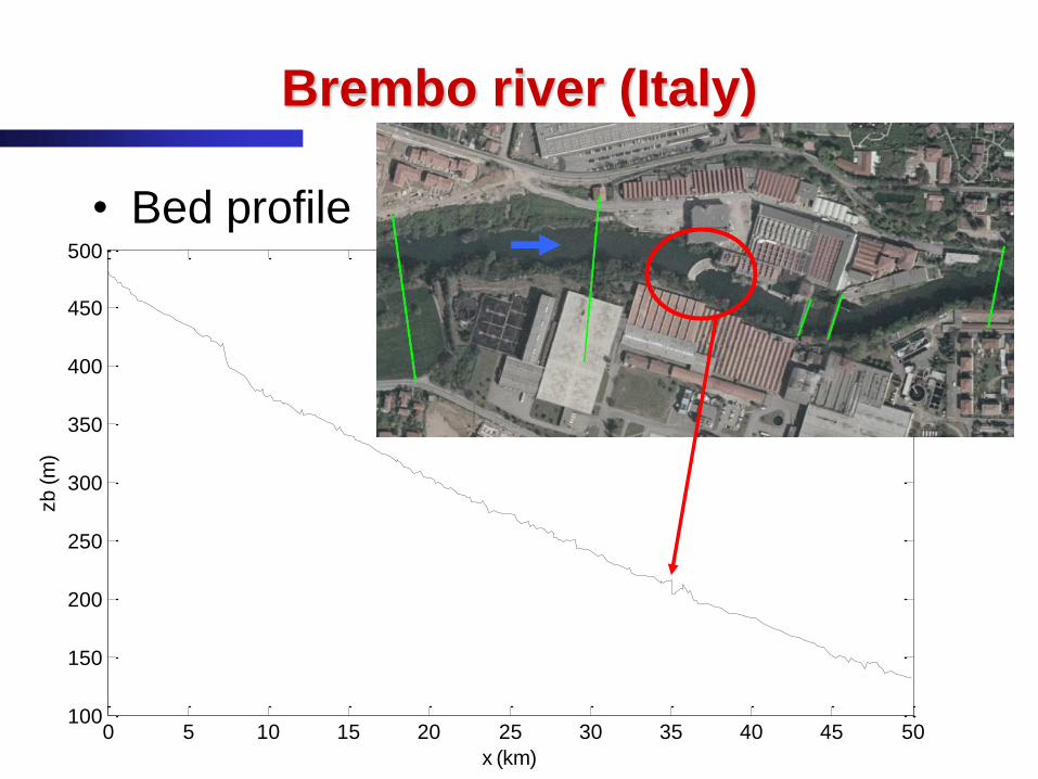
Brembo river (Italy)

• Bed profile

0 5 10 15 20 25 30 35 40 45 50100

150

200

250

300

350

400

450

500

x (km)

zb

(m

)

14

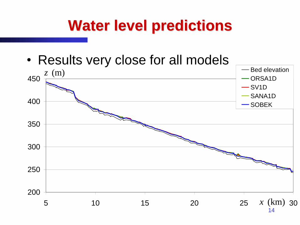
Water level predictions

200

250

300

350

400

450

5 10 15 20 25 30x (km)

z (m) Bed elevation

ORSA1D

SV1D

SANA1D

SOBEK

• Results very close for all models

15

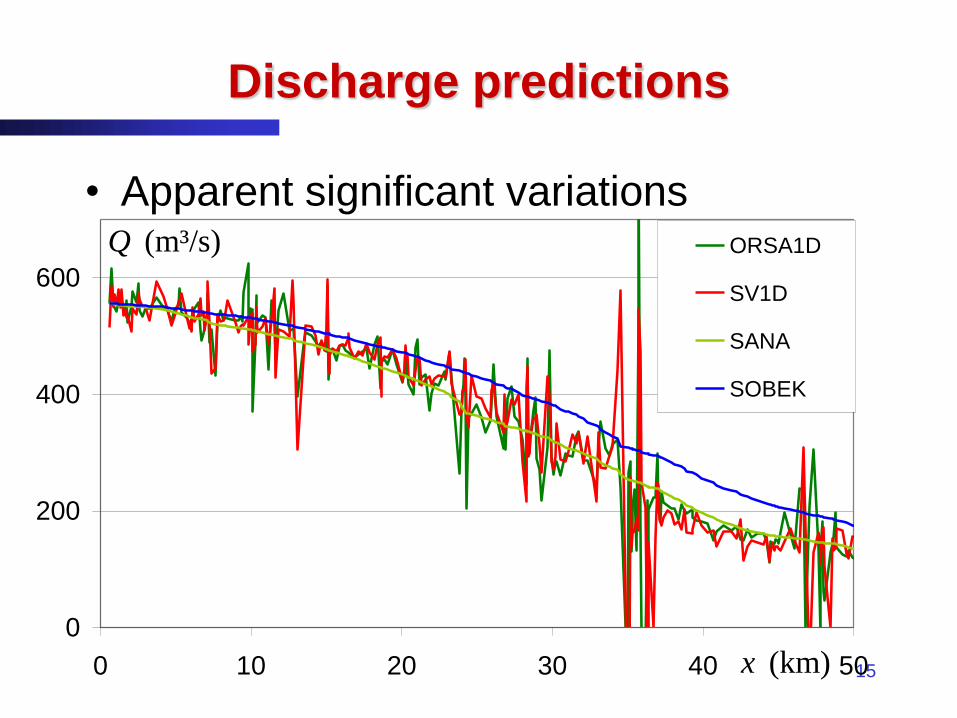
Discharge predictions

• Apparent significant variations

0

200

400

600

0 10 20 30 40 50x (km)

Q (m³/s) ORSA1D

SV1D

SANA

SOBEK

16

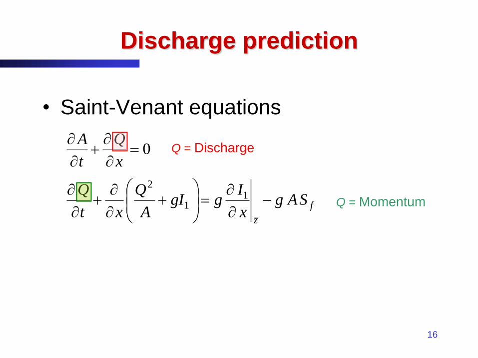
Discharge prediction

• Saint-Venant equations

f

z

SAgx

IggI

A

Q

xt

Q

x

Q

t

A

11

2

0 Q = Discharge

Q = Momentum

17 x

t

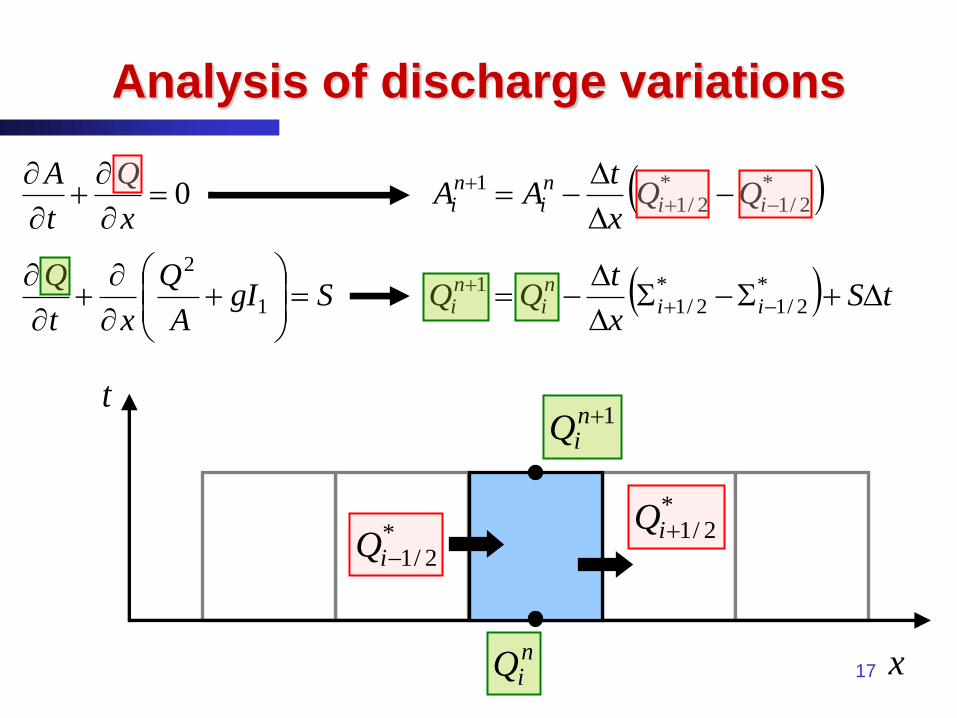
Analysis of discharge variations

niQ

1niQ

*2/1iQ

*2/1iQ

*2/1

*2/1

1

ii

ni

ni QQ

x

tAA

tSx

tQQ ii

ni

ni

*2/1

*2/1

1SgIA

Q

xt

Q

x

Q

t

A

1

2

0

18

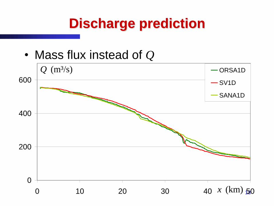
Discharge prediction

• Mass flux instead of Q

0

200

400

600

0 10 20 30 40 50x (km)

Q (m³/s) ORSA1D

SV1D

SANA1D

Open questions

• 1D approach: improved models

– HLLS

– Augmented-Roe with energy balance

19

Adaptation to irregular

cross-sections

Fabian Franzini,

PhD research

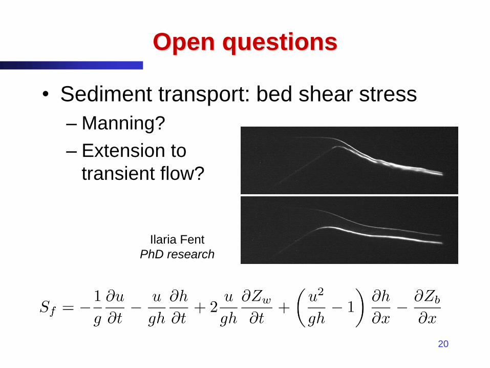
Open questions

• Sediment transport: bed shear stress

– Manning?

– Extension to

transient flow?

20

Ilaria Fent

PhD research

Open questions

• Sediment transport on steep slopes

– Gravity projection?

– Adapted transport formula?

21

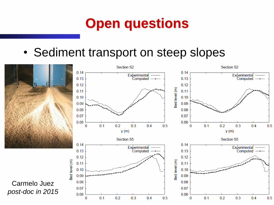
Open questions

• Sediment transport on steep slopes

22

Carmelo Juez

post-doc in 2015

Contents

• Mathematical models

• Open questions

– 1D approach

– Steep slopes

– Sediment transport

• Application to breaching

23

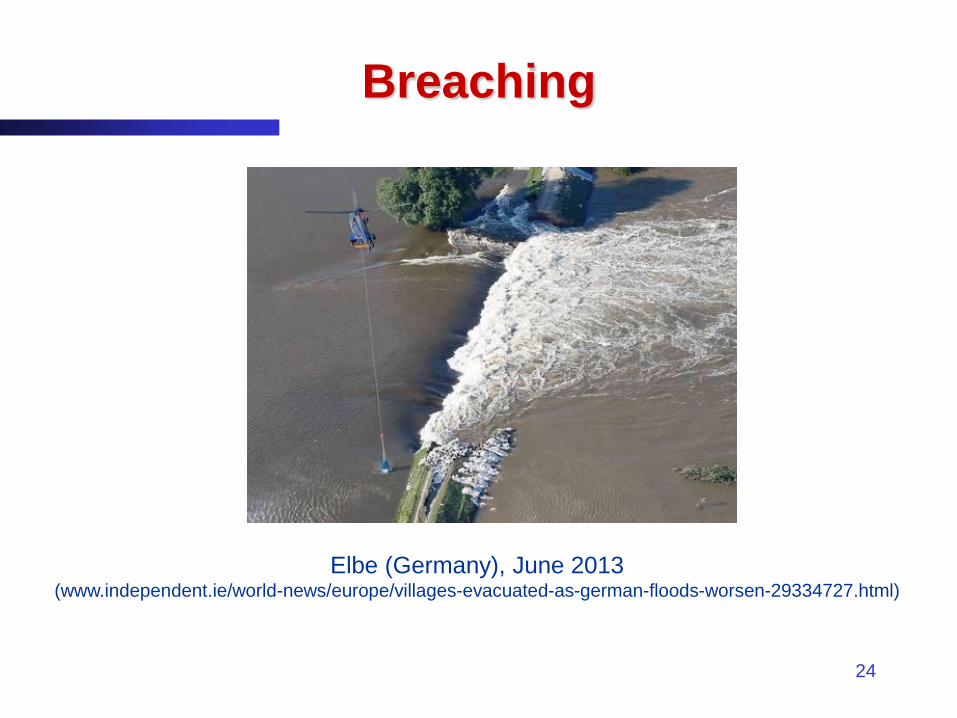
Breaching

24

Elbe (Germany), June 2013 (www.independent.ie/world-news/europe/villages-evacuated-as-german-floods-worsen-29334727.html)

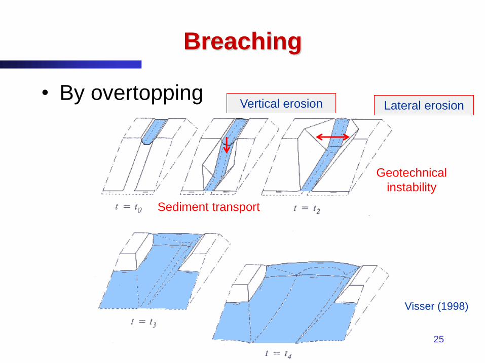
Breaching

• By overtopping

25

Visser (1998)

Vertical erosion Lateral erosion

Sediment transport

Geotechnical

instability

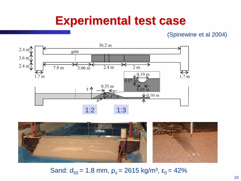
Experimental test case

• Dispositif expérimental

26

(Spinewine et al 2004)

Sand: d50 = 1.8 mm, ρs = 2615 kg/m³, ε0 = 42%

1:2

1:3

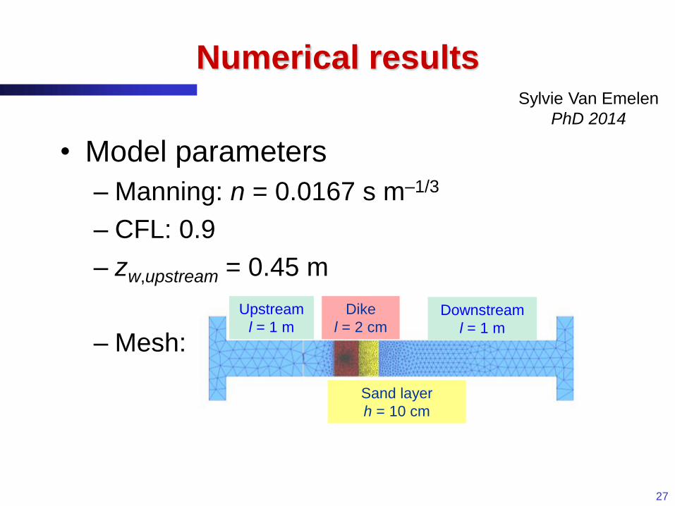
Numerical results

• Model parameters

– Manning: n = 0.0167 s m–1/3

– CFL: 0.9

– zw,upstream = 0.45 m

– Mesh:

27

Dike

l = 2 cm

Sand layer

h = 10 cm

Downstream

l = 1 m

Upstream

l = 1 m

Sylvie Van Emelen

PhD 2014

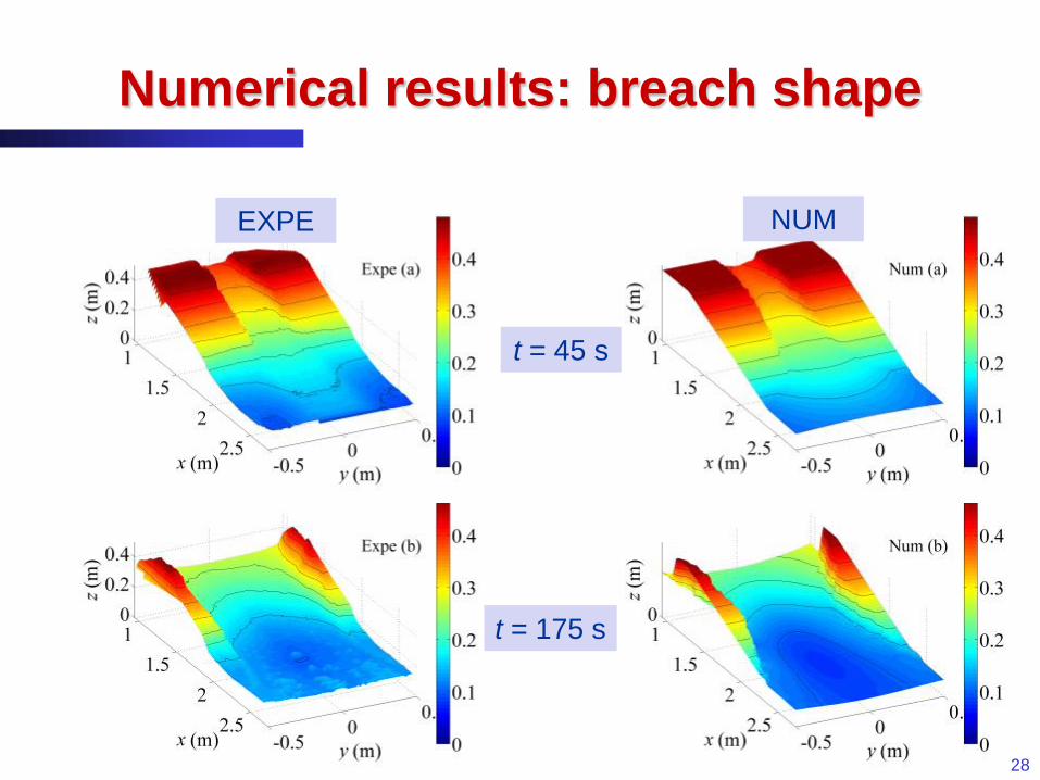
Numerical results: breach shape

28

t = 175 s

t = 45 s

EXPE NUM

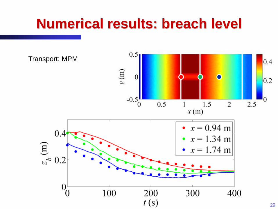
Numerical results: breach level

29

Transport: MPM

Dike:

variable mesh

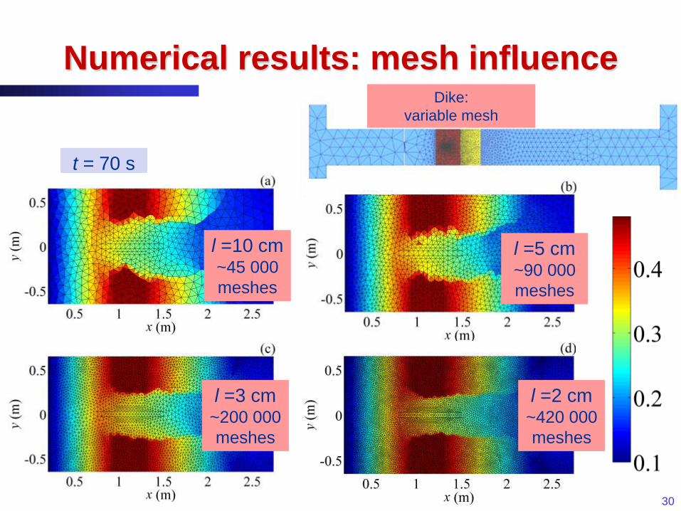
Numerical results: mesh influence

30

t = 70 s

l =10 cm ~45 000

meshes

l =5 cm ~90 000

meshes

l =3 cm ~200 000

meshes

l =2 cm ~420 000

meshes

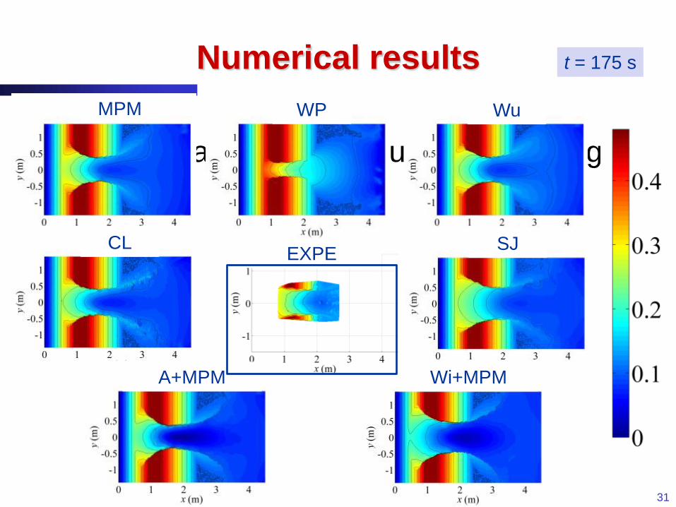
Numerical results

• Comparaison des formules de charriage

31

MPM

CL

WP Wu

SJ

Wi+MPM A+MPM

EXPE

t = 175 s

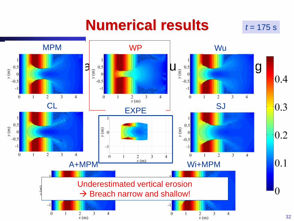
Numerical results

• Comparaison des formules de charriage

32

MPM

CL

WP Wu

SJ

Wi+MPM A+MPM

EXPE

t = 175 s

Underestimated vertical erosion

Breach narrow and shallow!

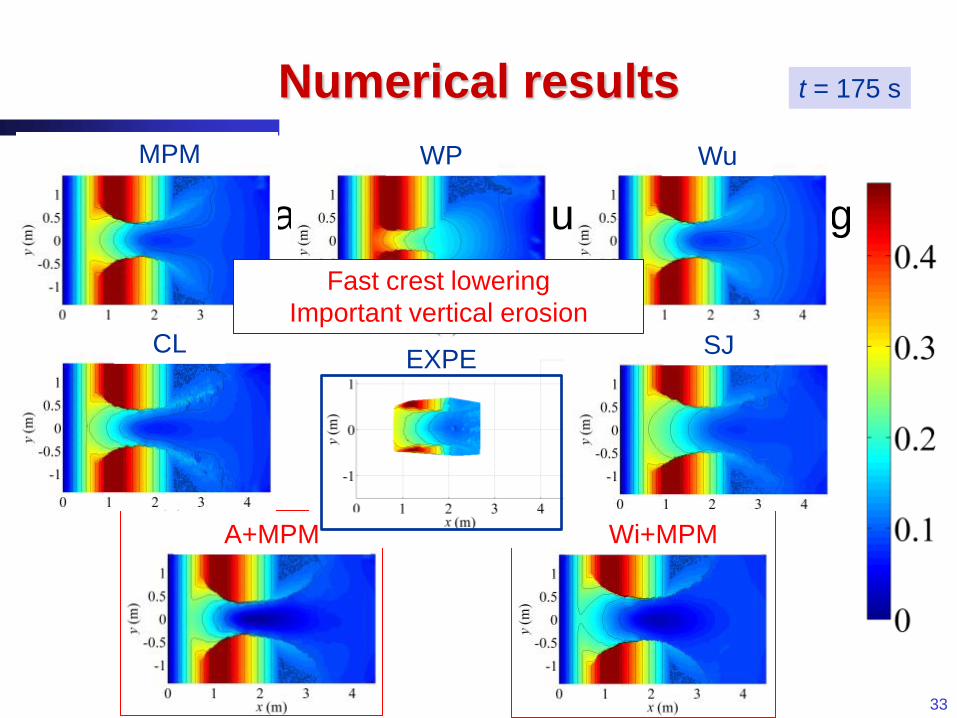
Numerical results

• Comparaison des formules de charriage

33

MPM

CL

WP Wu

SJ

Wi+MPM A+MPM

EXPE

t = 175 s

Fast crest lowering

Important vertical erosion

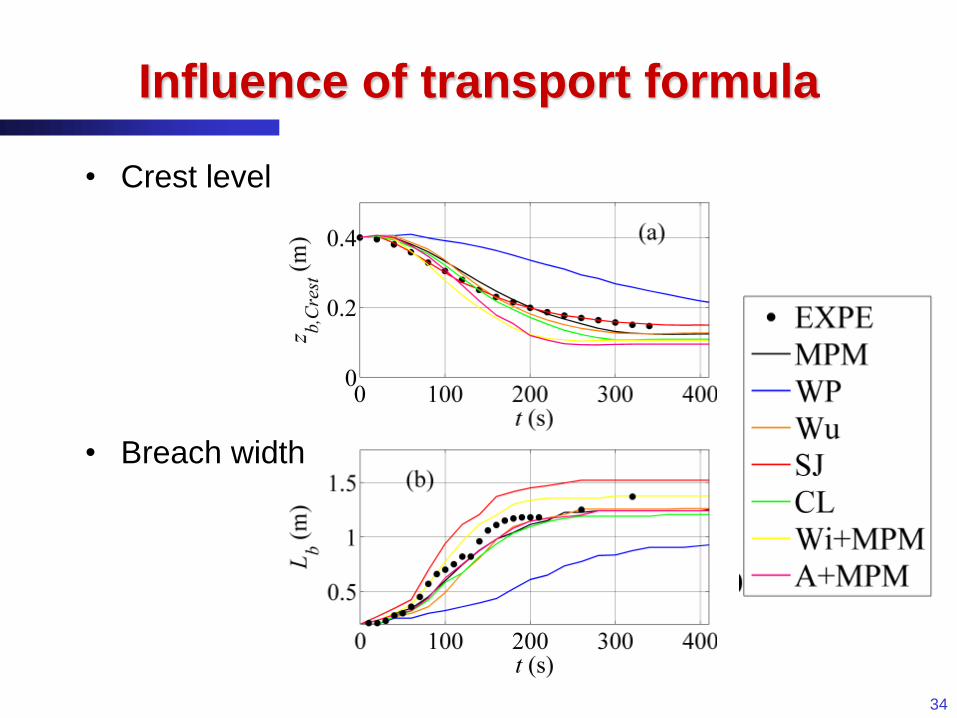
Influence of transport formula

34

• Crest level

• Breach width

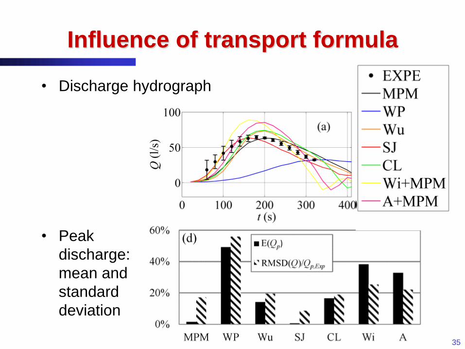
Influence of transport formula

35

• Discharge hydrograph

• Peak

discharge:

mean and

standard

deviation

Thank you for your attention !

36