State Estimation

Vipin Chandra Pandey

State Estimationassigning a value to an unknown system state variable based on

measurements from that system according to some criteria.

The process involves imperfect measurements that are redundant and the

process of estimating the system states is based on a statistical criterion

that estimates the true value of the state variables to minimize or maximize

the selected criterion.

Most Commonly used criterion for State Estimator in Power System is the

Weighted Least Square Criteria.

State & EstimateWhat’s A State?

The complete “solution” of the power system is known if all voltages and angles are identified at each bus. These quantities are the “state variables” of the system.

Why Estimate? Meters aren’t perfect. Meters aren’t everywhere. Very few phase measurements? SE suppresses bad measurements and uses the

measurement set to the fullest extent.2-3

State variable & Input to estimator In the Power System, The State Variables are the voltage Magnitudes and

Relative Phase Angles at the System Nodes.

The inputs to an estimator are imperfect power system measurements of

voltage magnitude and power, VAR, or ampere flow quantities.

The Estimator is designed to produce the “best estimate” of the system

voltage and phase angles, recognizing that there are errors in the measured

quantities and that they may be redundant measurements.

State Estimator output

Bus voltages, branch flows, …(state variables)

Measurement error processing results

Provide an estimate for all metered quantities

Filter out small errors due to model approximations

and measurement inaccuracies.

Detect and identify discordant measurements, the

so- called bad data.

Case 1 Suppose we use M13 and M32 and further suppose that M13 and M32 gives us perfect readings of the flows on their respective transmission lines.

M13=5 MW=0.05pu

M32 =40 MW=0.40pu

f13=1/x13*(1- 3 )=M13 = 0.05

f32=1/x32*(3- 2)=M32 = 0.40

Since 3=0 rad

1/0.4*(1- 0 )= 0.05

1/0.25*(0- 2) = 0.40

1 =0.02 rad

2 =-0.10 rad

Bus1Bus2

Bus3

60 MW

40 MW

65 MW

100 MW

Per unit Reactances

(100 MVA Base):

X12=0.2

X13=0.4

X23=0.25

M12

M13

M32

5 MWMeter Location

35 MW

Case1-Measurement with accurate meters)

Only two of these meter readings are required to calculate the bus phase angles and all load and generation values fully.

Case-2: use only M12 and M32.

M12=62 MW=0.62pu

M32 =37 MW=0.37pu

f12=1/x12*(1- 2 )=M12 = 0.62

f32=1/x32*(3- 2)=M32 = 0.37

Since 3=0 rad

1/0.2*(1- 2 )= 0.62

1/0.25*(0- 2) = 0.37

1 =0.0315 rad

2 =-0.0925 rad

Bus1Bus2

Bus3

62 MW

37 MW

65 MW

100 MW

Per unit Reactances

(100 MVA Base):

X12=0.2

X13=0.4

X23=0.25

M12

M13

M32

6 MW (7.875MW)Meter Location

35 MW

Case2-result of system flow. (M12 & M32)

Mismatch

Analysis of example

• use the measurements to estimate system conditions.• Measurements of were used to calculate the angles at different

buses by which all unmeasured power flows, loads, and generations can be calculated.

• voltage angles as the state variables for the three- bus system since knowing them allows all other quantities to be calculated

• If we can use measurements to estimate the “states” of the power system, then we can go on to calculate any power flows, generation, loads, and so forth that we desire.

Solution MethodologiesWeighted Least Square (WLS)method:

Minimizes the weighted sum of squares of the difference betweenmeasured and calculated values .

The weighted least-squares criterion, where the objective is to minimizethe sum of the squares of the weighted deviations of the estimated measurements, z, from the actual measurements, z.

Iteratively Reweighted Least SquareValue (WLAV)method:

(IRLS)Weighted Least Absolute

Minimizes the weighted sum of the absolute value ofdifferencebetween measured and calculated values.

The objective function to be minimized is given by

m| pi |

i 1

The weights get updated in every iteration.

m 1

e2

i2ii 1

(Cont.,)

The measurements are assumed to be in error: that is, the value obtained from the measurement device is close to the true value of the parameter being measured but differs by an unknown error.

If Zmeas be the value of a measurement as received from a measurement device.

If Ztrue be the true value of the quantity being measured. Finally, let η be the random measurement error.

Then mathematically it is expressed as

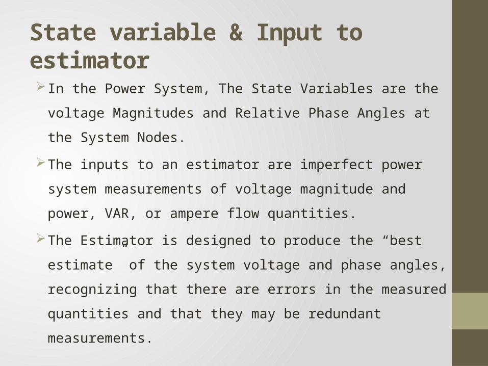
Probability density function

The random number, η, serves to model the uncertainty in the measurements.

If the measurement error is unbiased, the probability density function of η is usually chosen as a normal distribution with zero mean.

where σ is called the standard deviation and σ^2 is called the variance of the random number.

If σ is large, the measurement is relatively inaccurate (i.e., a poor-quality measurement device), whereas a small value of σ denotes a small error spread (i.e., a higher-quality measurement device).

Probability density function

Weighted least Squares-State Estimator

where

fi = function that is used to calculate the value being measured by the ith measurement

= variance for the ith measurement

J(x) = measurement residual

Nm = number of independent measurements

zmeas= ith measured quantity.

Note: that above equation may be expressed in per unit or in physical units such as MW, MVAR, or kV.

Estimate Ns unknown parameters using Nm measurements

Matrix Formulation:

If the functions are linear functions.

In vector form f(x)

Where

[H]=an Nm by Ns matrix containing the coefficients of the linear function

[H]=measurement function coefficients matrix

Nm= number of measurements

Ns=number of unknown parameters being estimated

[R]=covariance matrix of measurement error

The gradient of

Case Ns<Nm over determined

Case Ns=Nm completely determined

Case Ns>Nm underdetermined

Weighted Least Squares-Example

est 1

est 2x est

(Cont.,)

• To derive the [H] matrix, we need to write the measurementsas a function of the state variablesare written in per unit as

2 . These functions1 and

12 12 1 2 1 2

13 13 1 3 1

32 32 3 2 2

1(M f ) 5 5

0.2

1(M f ) 2.5

0.41

M f ( ) 40.25

(Cont.,)

55

2.5 0

04

[H]

2M12

2M12

2M13

2M13

2M32

2M32

0.0001

R 0.0001

0.0001

(Cont.,)

•

11

est 1

est 2

1

0.0001 55

2.5 0

04

5 2.5 0

-5 0 -40.0001

0.0001

0.0001 0.62

0.06

0.37

5 2.5 0

-5 0 -40.0001

0.0001

(Cont.,)

• We get

• From the estimated phase angles, we can calculate the power flowing in each transmission line and the net generation or load at each bus.

est 1

est 2

0.028571

0.094286

5 ))2 (0.06 (2.5 ))2 (0.37 (4 ))2 1 2

0.00012.14

1

0.0001 2

0.0001J( 1, 2 )

(0.62 (5

Solution of the weighted least square example

Application of State Estimation

To provide a view of real-time power system conditions Real-time data primarily come from SCADA SE supplements SCADA data: filter, fill, smooth.

To provide a consistent representation forpower system security analysis• On-line dispatcher power flow• Contingency Analysis• Load Frequency Control

To provide diagnostics for modeling & maintenance

ReferencesPower generation operation and control by Allen J.Wood &

Bruce F.WollenbergOperation and control in Power systems by P.S.R. Murthy

THANK YOU