Transient Analysis of Grounding Systems Without Computer

L. Grcev, B. Markovski Ss. Cyril and Methodius University

Faculty of Electrical Engineering & IT Skopje, Republic of Macedonia

Leonid.Grcev@ieee.org , bmarkovski@feit.ukim.edu.mk

V. Arnautovski-Toseva, K. E. K. Drissi Blaise Pascal University

Institute Pascal, LASMEA Clermont-Ferrand, France

Vesna.ARNAUTOVSKI@lasmea.univ-bpclermont.fr

Abstract—Recently simple empirical formulas have been introduced that estimate the impulse impedance, impulse coefficient and effective length/area of different arrangements of grounding electrodes (horizontal and vertical electrodes and grounding grids) under typical lightning currents. Soil ionization and inductive effects are both included in the formulas for smaller simple arrangements of grounding electrodes, while soil ionization is ignored for grounding grids. To illustrate and validate the new formulas, we compare the results from the formulas with experimental data recently published by different research groups.

Keywords-grounding; lightning; modeling

I. INTRODUCTION The quantities that are usually used to characterize the

dynamic behavior of the grounding electrode during lightning discharge are: impulse impedance, impulse coefficient and effective length/area [1]–[4].

We consider the current pulse that is injected into the grounding system and the resulting electric potential at the injection point in relation to the remote ground. The impulse impedance

( )i t( )v t

Z is defined as:

m

m

VZ

I= , (1)

where mI and are the peak values of and , respectively. To compare the grounding performance under surge conditions with the performance at a power frequency,

mV ( )i t ( )v t

Z is related to the power frequency grounding resistance R through the dimensionless impulse coefficient A :

ZAR

= . (2)

Values of A larger than one indicate impaired surge performance as compared with the LF grounding performance, while values of A equal to or less than one indicate equivalent or superior surge performance, respectively.

For longer grounding electrodes or larger grounding grids, Z might become larger than R – that is, A might become larger than one. Consequently, the surge effective length of electrodes or size length of square effective area a of grounding grids are defined as the maximal electrode length or maximal side length of square area of grounding grids, respectively, for which

eff

eff

A is equal to one [1]–[4].

II. FORMULAS FOR IMPULSE COEFFICIENT Details on development and validation of new empirical

formulas for lightning surge characteristics of simple grounding electrodes arrangements and grounding grids can be found elsewhere (see [1]–[3] for grounding electrodes and [4] for grids); here we include only brief summary for completeness.

A. Grounding electrode First we compute the impulse coefficient 0A when

frequency dependent inductive effects are taken into account but soil ionization is ignored. Next the ionization is taken into account and complete impulse coefficient A is computed.

The first step is to compute the coefficients α and β :

, 0.25710.025 exp 0.82 ( )Tα ⎡ ⎤= + − ⋅ ⋅⎣ ⎦ρ

ρ . (3) 0.55510.17 exp 0.22 ( )Tβ ⎡ ⎤= + − ⋅ ⋅⎣ ⎦

Here, ρ is the soil resistivity (in ohmmeters), and T1 is current pulse zero-to-peak time (in microseconds). Next, the effective length (in meters) is determined by: eff

1

effβ

α−

= . (4)

When the length of the grounding electrode (in meters) is less or equal than then the impulse coefficient is assumed equal to one:

eff

This work was supported in part by the FP7-PEOPLE-2009-IEF Project 253783, the Republic of Macedonia Ministry of Education and Science, and the Macedonian Academy of Sciences and Arts.

978-1-4673-1897-6/12/$31.00 ©2012 IEEE

2012 International Conference on Lightning Protection (ICLP), Vienna, Austria

. (5) 0 1, ( )effA = ≤

For the electrode length , dependence of the

impulse coefficient eff≥

0A on is nearly linear and may be approximated by:

0 , ( )effA α β= + ≥ . (6)

Effects of soil ionization are negligible if

m gI I<< , (7)

where gI (in kiloamperes) is computed by:

022g

EI

Rρ

π= . (8)

Here, (in kilovolts per meter) is the critical electric field intensity ( = 300 kV/m according to [5]), and R is LF resistance to ground. For vertical rod following popular formula can be used

0E

0E

4ln 1 , ( )

2R a

aρπ

⎡ ⎤⎛ ⎞= −⎜ ⎟⎢ ⎥⎝ ⎠⎣ ⎦>> , (9)

and for horizontal electrode

2ln 1 , ( , )2

Rad

ρπ

⎡ ⎤⎛ ⎞= − >> <<⎢ ⎥⎜ ⎟

⎝ ⎠⎣ ⎦a d . (10)

Here a (in meters) is electrode radius, and d (in meters) is depth of burial.

In case when the effects of soil ionization are negligible the impulse coefficient is

0A A= , (11)

where 0A is given by (5) or (6).

Impulse coefficient A that takes into account the time dependent non-linear soil ionization effects (and in the same time the frequency dependent inductive effects) is determined by:

01 1

1 m g

A AI I

= ++

− . (12)

Here 0A is computed using (5) or (6), mI (in kiloamperes) is the lightning current pulse peak value and gI is computed by (8).

The list of input parameters and their validity ranges for the formulas (3)–(12) is given in Table I.

Presented formulas can also be applied for additional arrangements of grounding electrodes, such as, centrally fed

horizontal electrode, cross electrodes and two or four rods, using reduction factors given in Table III on p. 447 of reference [1].

TABLE I. INPUT PARAMETERS OF THE FORMULAS (3)–(12).

Parameter Symbol Unit Validity range

Electrode length m 3 – 30

Soil resistivity ρ Ωm 10 – 1000

Current pulse zero-to-peak time

T1 μs 0.2 – 10

Current pulse peak value mI kA 0 – 100

Soil’s critical E field 0E kV/m 300 – 1000

B. Grounding grid We consider a square grounding grid with side length a (in

meters). We compute the effective area that is also assumed as a square area around the current feed point. The formula for the side length of the effective area (in meters) is effa

, (13) ( )0.221exp 0.84effa K Tρ⎡= ⋅ ⋅⎣

⎤⎦

Here, 1K = for a center-fed grid, and for a corner-fed grid. Units and ranges of other parameters in (13) are given in Table II.

0.5K =

When the grid side a (in meters) is smaller than the side of the effective area a , we approximate the value of the impulse coefficient by

eff

( )1, effA a a= ≤ . (14)

For equal to and larger than , the impulse coefficient is approximated by

a effa

( ), effeff

aA a aa

= ≥ . (15)

Input parameters for the proposed formulas (13)–(15) and their validity ranges are given in Table II.

TABLE II. INPUT PARAMETERS OF THE FORMULAS (13)–(15).

Parameter Symbol Unit Validity range

Square grid side length a m 5 – 100

Soil resistivity ρ Ωm 10 – 1000

Current pulse zero-to-peak time

T1 μs 0.2 – 10

III. COMPARISON WITH EXPERIMENTAL RESULTS

A. Simple grounding electrodes arrangements 1) High current measurements by Geri [6]

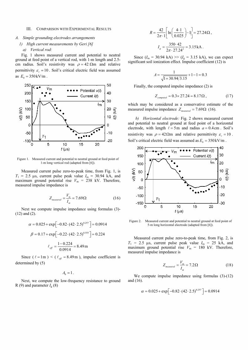
a) Vertical rod: Fig. 1 shows measured current and potential to neutral

ground at feed point of a vertical rod, with 1-m length and 2.5-cm radius. Soil’s resistivity was 42 mρ = Ω and relative permittivity 10rε = . Soil’s critical electric field was assumed as . 0 350E = kV/m

Figure 1. Measured current and potential to neutral ground at feed point of 1-m long vertical rod (adapted from [6]).

Measured current pulse zero-to-peak time, from Fig. 1, is T1 = 2.5 μs, current pulse peak value Im = 30.94 kA, and maximum ground potential rise Vm = 238 kV. Therefore, measured impulse impedance is

7.69mmeasured

m

VZ

I= = Ω (16)

Next we compute impulse impedance using formulas (3)-(12) and (2).

0.2570.025 exp 0.82 (42 2.5) 0.0914α ⎡ ⎤= + − ⋅ ⋅ =⎣ ⎦

0.5550.17 exp 0.22 (42 2.5) 0.224β ⎡ ⎤= + − ⋅ ⋅ =⎣ ⎦

1 0.224 8.49m0.0914eff−

= =

Since ( ) < ( ), impulse coefficient is determined by (5)

1m= 8.49meff =

0 1A = .

Next, we compute the low-frequency resistance to ground R (9) and parameter Ig (8)

42 4 1ln 1 27.242 1 0.025

Rπ

⎡ ⋅ ⎤⎛ ⎞= − = Ω⎜ ⎟⎢ ⎥⋅ ⎝ ⎠⎣ ⎦,

2

350 42 3.15kA2 27.24gIπ

⋅= =

⋅.

Since (Im = 30.94 kA) >> (Ig = 3.15 kA), we can expect significant soil ionization effect. Impulse coefficient (12) is

1 1 1 0.31 30.94 3.15

A = + −+

=

Finally, the computed impulse impedance (2) is

0.3 27.24 8.17computedZ = × = Ω

Ω

, (17)

which may be considered as a conservative estimate of the measured impulse impedance (16). 7.69measuredZ =

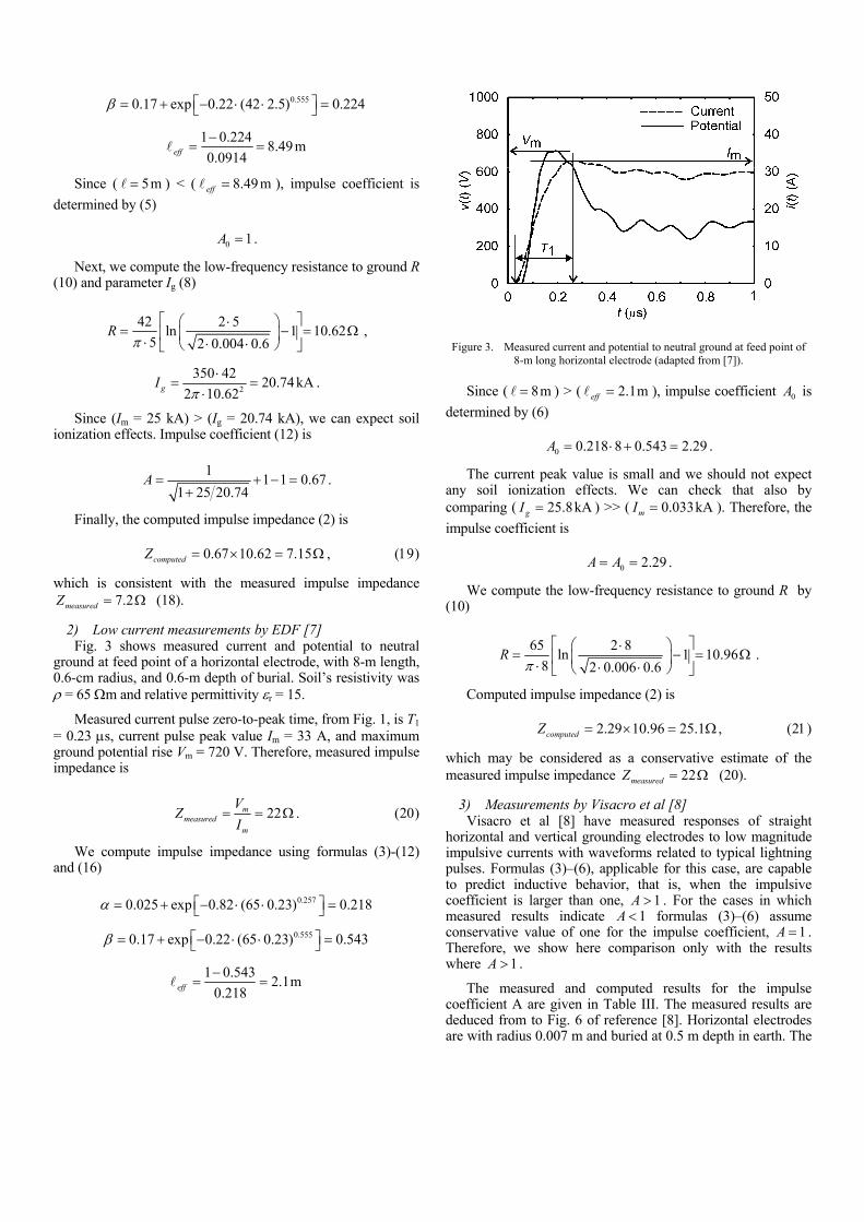
b) Horizontal electrode: Fig. 2 shows measured current and potential to neutral ground at feed point of a horizontal electrode, with length 5m= and radius 0.4cma = . Soil’s resistivity was 42 mρ = Ω and relative permittivity 10rε = . Soil’s critical electric field was assumed as m . 0 350kV/E =

Figure 2. Measured current and potential to neutral ground at feed point of 5-m long horizontal electrode (adapted from [6]).

Measured current pulse zero-to-peak time, from Fig. 2, is

T1 = 2.5 μs, current pulse peak value Im = 25 kA, and maximum ground potential rise Vm = 180 kV. Therefore, measured impulse impedance is

7.2mmeasured

m

VZ

I= = Ω (18)

We compute impulse impedance using formulas (3)-(12) and (16).

0.2570.025 exp 0.82 (42 2.5) 0.0914α ⎡ ⎤= + − ⋅ ⋅ =⎣ ⎦

0.5550.17 exp 0.22 (42 2.5) 0.224β ⎡ ⎤= + − ⋅ ⋅ =⎣ ⎦

1 0.224 8.49m0.0914eff−

= =

Since ( ) < ( ), impulse coefficient is determined by (5)

5m= 8.49meff =

0 1A = .

Next, we compute the low-frequency resistance to ground R (10) and parameter Ig (8)

42 2 5ln 1 10.625 2 0.004 0.6

Rπ

⎡ ⎤⋅⎛ ⎞= −⎢ ⎥⎜ ⎟⋅ ⋅ ⋅⎝ ⎠⎣ ⎦

= Ω ,

2

350 42 20.74kA2 10.62gIπ

⋅= =

⋅.

Since (Im = 25 kA) > (Ig = 20.74 kA), we can expect soil ionization effects. Impulse coefficient (12) is

1 1 1 0.671 25 20.74

A = + −+

=

Ω

.

Finally, the computed impulse impedance (2) is

, (19) 0.67 10.62 7.15computedZ = × =

which is consistent with the measured impulse impedance (18). 7.2measuredZ = Ω

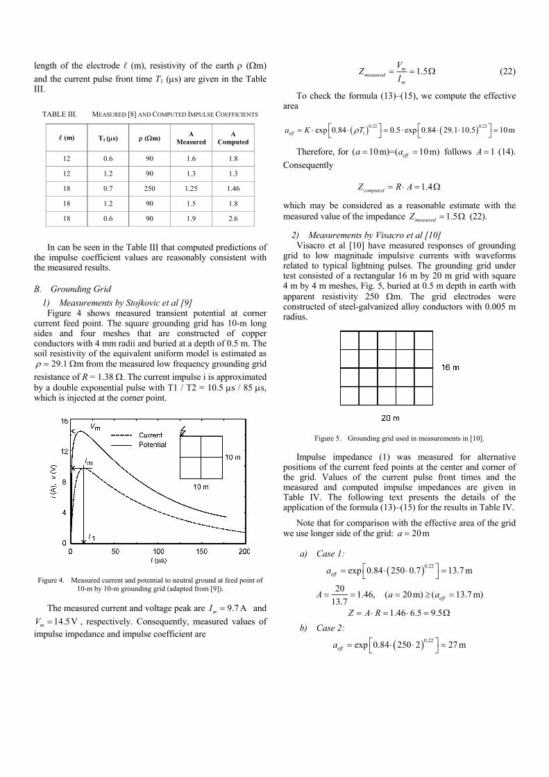
2) Low current measurements by EDF [7] Fig. 3 shows measured current and potential to neutral

ground at feed point of a horizontal electrode, with 8-m length, 0.6-cm radius, and 0.6-m depth of burial. Soil’s resistivity was ρ = 65 Ωm and relative permittivity εr = 15.

Measured current pulse zero-to-peak time, from Fig. 1, is T1 = 0.23 μs, current pulse peak value Im = 33 A, and maximum ground potential rise Vm = 720 V. Therefore, measured impulse impedance is

22mmeasured

m

VZ

I= = Ω . (20)

We compute impulse impedance using formulas (3)-(12) and (16)

0.2570.025 exp 0.82 (65 0.23) 0.218α ⎡ ⎤= + − ⋅ ⋅ =⎣ ⎦

0.5550.17 exp 0.22 (65 0.23) 0.543β ⎡ ⎤= + − ⋅ ⋅ =⎣ ⎦

1 0.543 2.1m0.218eff−

= =

Figure 3. Measured current and potential to neutral ground at feed point of 8-m long horizontal electrode (adapted from [7]).

Since ( 8m= ) > ( 2.1meff = ), impulse coefficient 0A is determined by (6)

0 0.218 8 0.543 2.29A = ⋅ + = .

The current peak value is small and we should not expect any soil ionization effects. We can check that also by comparing ( 25.8kAgI = ) >> ( ). Therefore, the impulse coefficient is

0.033kAmI =

0 2.29A A= = .

We compute the low-frequency resistance to ground R by (10)

65 2 8ln 1 10.96

8 2 0.006 0.6R

π⎡ ⎤⋅⎛ ⎞

= − = Ω⎢ ⎥⎜ ⎟⋅ ⋅ ⋅⎝ ⎠⎣ ⎦.

Computed impulse impedance (2) is

2.29 10.96 25.1computedZ = × = Ω , (21)

which may be considered as a conservative estimate of the measured impulse impedance (20). 22measuredZ = Ω

3) Measurements by Visacro et al [8] Visacro et al [8] have measured responses of straight

horizontal and vertical grounding electrodes to low magnitude impulsive currents with waveforms related to typical lightning pulses. Formulas (3)–(6), applicable for this case, are capable to predict inductive behavior, that is, when the impulsive coefficient is larger than one, 1A >

1. For the cases in which

measured results indicate A < formulas (3)–(6) assume conservative value of one for the impulse coefficient, 1A = . Therefore, we show here comparison only with the results where 1A > .

The measured and computed results for the impulse coefficient A are given in Table III. The measured results are deduced from to Fig. 6 of reference [8]. Horizontal electrodes are with radius 0.007 m and buried at 0.5 m depth in earth. The

length of the electrode (m), resistivity of the earth ρ (Ωm) and the current pulse front time T1 (μs) are given in the Table III.

TABLE III. MEASURED [8] AND COMPUTED IMPULSE COEFFICIENTS

(m) T1 (μs) ρ (Ωm) A Measured

A Computed

12 0.6 90 1.6 1.8

12 1.2 90 1.3 1.3

18 0.7 250 1.25 1.46

18 1.2 90 1.5 1.8

18 0.6 90 1.9 2.6

In can be seen in the Table III that computed predictions of the impulse coefficient values are reasonably consistent with the measured results.

B. Grounding Grid 1) Measurements by Stojkovic et al [9]

Figure 4 shows measured transient potential at corner current feed point. The square grounding grid has 10-m long sides and four meshes that are constructed of copper conductors with 4 mm radii and buried at a depth of 0.5 m. The soil resistivity of the equivalent uniform model is estimated as

29.1 mρ = Ω from the measured low frequency grounding grid resistance of R = 1.38 Ω. The current impulse i is approximated by a double exponential pulse with T1 / T2 = 10.5 μs / 85 μs, which is injected at the corner point.

Figure 4. Measured current and potential to neutral ground at feed point of 10-m by 10-m grounding grid (adapted from [9]).

The measured current and voltage peak are and , respectively. Consequently, measured values of

impulse impedance and impulse coefficient are

9.7 AmI =14.5VmV =

1.5mmeasured

m

VZ

I= = Ω (22)

To check the formula (13)–(15), we compute the effective area

( ) ( )0.22 0.221exp 0.84 0.5 exp 0.84 29.1 10.5 10meffa K Tρ⎡ ⎤ ⎡ ⎤= ⋅ ⋅ = ⋅ ⋅ ⋅ =⎣ ⎦ ⎣ ⎦

Therefore, for ( 10 m)=( 10 m)effa a= = follows 1A = (14). Consequently

1.4computedZ R A= ⋅ = Ω

which may be considered as a reasonable estimate with the measured value of the impedance (22). 1.5measuredZ = Ω

2) Measurements by Visacro et al [10] Visacro et al [10] have measured responses of grounding

grid to low magnitude impulsive currents with waveforms related to typical lightning pulses. The grounding grid under test consisted of a rectangular 16 m by 20 m grid with square 4 m by 4 m meshes, Fig. 5, buried at 0.5 m depth in earth with apparent resistivity 250 Ωm. The grid electrodes were constructed of steel-galvanized alloy conductors with 0.005 m radius.

Figure 5. Grounding grid used in measurements in [10].

Impulse impedance (1) was measured for alternative positions of the current feed points at the center and corner of the grid. Values of the current pulse front times and the measured and computed impulse impedances are given in Table IV. The following text presents the details of the application of the formula (13)–(15) for the results in Table IV.

Note that for comparison with the effective area of the grid we use longer side of the grid: 20ma =

a) Case 1:

( )0.22exp 0.84 250 0.7 13.7 meffa ⎡ ⎤= ⋅ ⋅ =⎣ ⎦

20 1.46, ( 20m) ( 13.7 m)13.7 effA a a= = = ≥ =

1.46 6.5 9.5Z A R= ⋅ = ⋅ = Ω b) Case 2:

( )0.22exp 0.84 250 2 27 meffa ⎡ ⎤= ⋅ ⋅ =⎣ ⎦

• Earth resistivity – from 10 to 100 Ωm. 1, ( 20m) ( 27 m)effA a a= = < = 6.5Z A R= ⋅ = Ω • Current pulse zero-to-peak time – from 0.2 to 10 μs.

c) Case 3: • Current pulse peak value – up to 100 kA. ( )0.22exp 0.84 250 4 46.5meffa ⎡ ⎤= ⋅ ⋅ =⎣ ⎦ Formulas are capable to approximately estimate

impairment of the grounding transient performance in comparison to the LF performance in the first moments of the stroke due to the inductive effects. In case of current pulses with high magnitudes, simultaneously with the frequency dependent inductive effects, formulas estimate the improvement of the performance due to the non-linear earth ionization.

1, ( 20 m) ( 46.5m)effA a a= = < = 6.5Z A R= ⋅ = Ω

d) Case 4:

( )0.220.5 exp 0.84 250 0.7 6.85meffa ⎡ ⎤= ⋅ ⋅ ⋅ =⎣ ⎦

20 2.92, ( 20m) ( 6.85m)6.85 effA a a= = = ≥ = The presented empirical formulas have been deducted from

simulations using the electromagnetic field model for transients in grounding systems that has been previously compared with experiments.

2.92 6.5 19Z A R= ⋅ = ⋅ = Ω e) Case 5:

Presented comparisons between the results from the formulas and experimental data available in the literature demonstrate their ability to predict dynamic characteristics of grounding systems, which suggests that they may be used for the first check in lightning performance calculations. For more accurate computations and more complex situations use of computer software might be necessary.

( )0.220.5 exp 0.84 250 2 13.5meffa ⎡ ⎤= ⋅ ⋅ ⋅ =⎣ ⎦

20 1.48, ( 20 m) ( 13.5m)13.5 effA a a= = = ≥ =

1.48 6.5 9.6Z A R= ⋅ = ⋅ = Ω f) Case 6:

( )0.220.5 exp 0.84 250 4 23meffa ⎡ ⎤= ⋅ ⋅ ⋅ =⎣ ⎦ REFERENCES

1, ( 20 m) ( 23m)effA a a= = < = [1] L. Grcev, “Impulse efficiency of ground electrodes”, IEEE Trans. Power Del., vol. 24, no. 1, pp. 441-451, Jan. 2009. 6.5Z A R= ⋅ = Ω

[2] L. Grcev, “Modeling of grounding electrodes under lightning currents”, IEEE Trans. Electromagn. Compat., vol. 51, no. 3, pp. 559-571, Aug. 2009. TABLE IV. MEASURED [10] AND COMPUTED IMPULSE IMPEDANCES

Case Position of

current feed point

T1 (μs) Z (Ω) Measured

Z (Ω) Computed

1 0.7 10 9.5

2 2 5.8 6.5

3

Center

4 5.3 6.5

4 0.7 21 19

5 2 9.5 9.6

6

Corner

4 6.9 6.5

[3] L. Grcev, “Time- and frequency-dependent lightning surge characteristics of grounding electrodes”, IEEE Trans. Power Del., vol. 24, no. 4, pp. 2186-2196, October 2009.

[4] L. Grcev, “Lightning surge efficiency of grounding grids,” IEEE Trans. Power Del., vol. 26, no. 3, pp. 1692-1699, Jul 2011.

[5] IEEE modeling and analysis of system transients Working Group, Fast front transients Task Force, “Modeling guidelines for fast front transients”, IEEE Trans. Power Del., vol. 11, no. 1, pp. 493-506, Jan. 1996.

[6] A. Geri, “Behaviour of grounding systems excited by high impulse currents: the model and its validation”, IEEE Trans. Power Del., vol. 14, no. 3, pp. 1008-1017, Jul. 1999.

[7] H. Rochereau, B. Merheim, “Application of the transmission lines theory and EMTP program for modelisation of grounding systems in high frequency range”, Collection de notes internes de la Direction des Etudes et Recherches, Electricité de France, 93NR00059, pp. 1-31, Paris, May 1993.

IV. CONCLUSIONS [8] S. Visacro and G. Rosado, “Response of grounding electrodes to

impulsive currents: An experimental evaluation,” IEEE Trans. Electromagn. Compat., vol. 51, no. 1, pp. 161–164, Feb. 2009.

Paper describes application of simple formulas for impulse impedance, impulse coefficient and effective length/area for typical lightning current waveforms for following range of parameters:

[9] Z. Stojkovic, M. S. Savic, J. M. Nahman, D. Salamon and B. Bukorovic, “Sensitivity analysis of experimentally determined grounding grid impulse characteristics”, IEEE Trans. Power Del., vol. 13, no. 4, pp. 1136–1142, Oct. 1998. • Simple arrangements of grounding electrodes, such as:

simple horizontal and vertical electrodes, center-fed horizontal and cross electrodes, two and four rods, with dimensions up to 30 m.

[10] S. Visacro, M. B. Guimaraes N., R. A. Araujo, L. S. de Araujo, “Experimental impulse response of grounding grids”, Proc. of 7th Asia-Pacific Int. Conf. on Lightning, pp. 637-641, Chengdu, China, November 2011.

• Grounding grids – square grids with side lengths up to 100 m.