Water demand forecasting

Chapter 4: Design of Water Supply

Pipe Network

Dr. Mohsin Siddique

Assistant Professor

1

Hydraulics

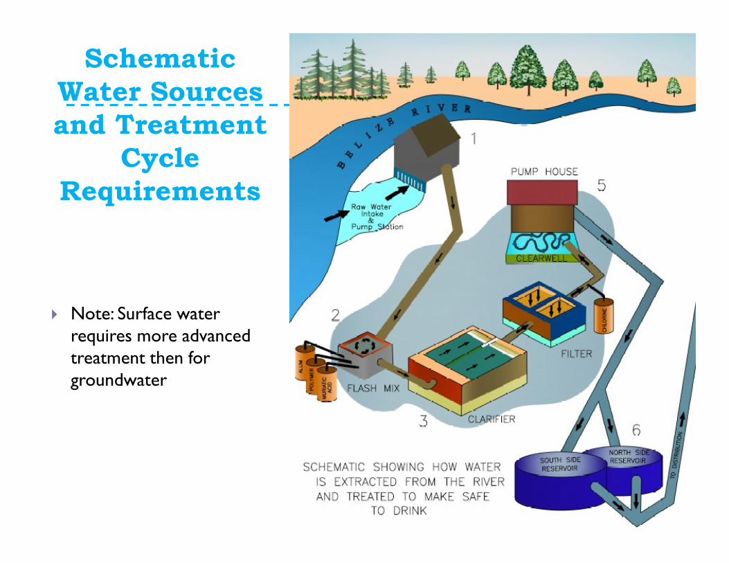
Schematic

Water Sources

and Treatment

Cycle

Requirements

� Note: Surface water requires more advanced treatment then for groundwater

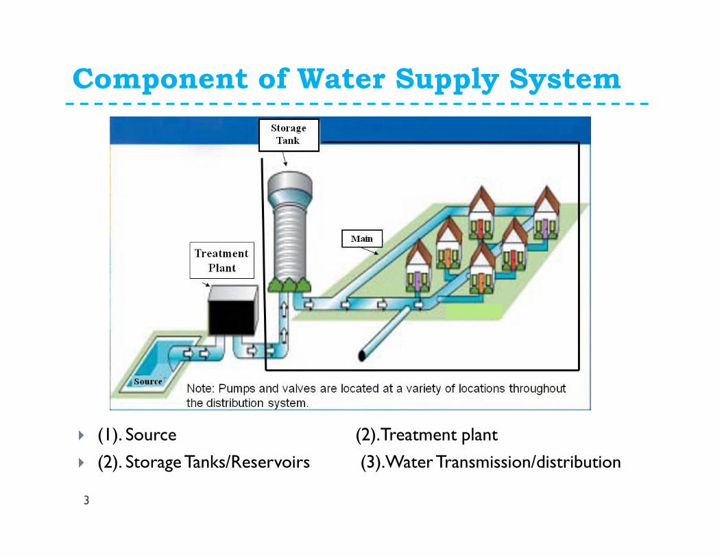
Component of Water Supply System

3

� (1). Source (2).Treatment plant

� (2). Storage Tanks/Reservoirs (3).Water Transmission/distribution

Design of Water Distribution System

� A municipal water distribution system is used to deliver water to the consumer.

� Water is withdrawn from along the pipes in a pipe network system (for computational purposes all demands on the system are assumed to occur at the junction nodes)

� Pressure is the main concern in a water distribution system. At no time should the water pressure in the system be so low that contamination (e.g. contaminated groundwater) could enter the system at points of leakage

� The total water demand at each node/Junction is estimated from residential, industrial and commercial water demands at that node. The fire flow is added to account for emergency water demand

Water Demand Forecasting/Estimation

� In the planning of municipal water-supply projects, the water demand at the end of the design life of the project is usually the basis for design.

� For existing water-supply systems, the American Water Works Association (AWWA, 1992) recommends that every 5 or 10 years, as a minimum, water-distribution systems be thoroughly reevaluated for requirements that would be placed on it by development and reconstruction over a 20-year period into the future.

� The estimation of the design flowrates for components of the water-supply system typically requires forecast of the population of the service area at the end of the design life, which is then multiplied by the per capita water demand to yield the design flowrate.

� Whereas the per capita water demand can usually be assumed to be fairly constant, the estimation of the future population typically involves a nonlinear extrapolation of past population trends.

Domestic Population Forecasting

6

� Design of water supply and sanitation scheme is based on the projected population of a particular city, estimated for the design period.

� Any underestimated value will make system inadequate for the purpose intended; similarly overestimated value will make it costly.

� Change in the population of the city over the years occurs, and the system should be designed taking into account of the population at the end of the design period.

� The present and past population record for the city can be obtained from the census population records. After collecting these population figures, the population at the end of design period is predicted using various methods as suitable for that city considering the growth pattern followed by the city.


7

� Methods of population forecasting

� Arithmetic increase method

� Geometrical increase method

� Incremental increase method

� Graphical method

� Comparative graphical method

� Master plan method

� Logistic curve method

� Ratio method etc


Arithmetic increase method

8

� This method is suitable for large and old city with considerable development.

� In this method the average increase in population per decade is calculated from the past census reports. This increase is added to the present population to find out the population of the next decade. Thus, it is assumed that the population is increasing at constant rate.

� Hence, dP/dt = C i.e. rate of change of population with respect to time is constant.

� Therefore, Population after nth decade will be

Pn= P + n.C

� Where, Pn is the population after n decades and P is present population.


Geometric Increase Method

9

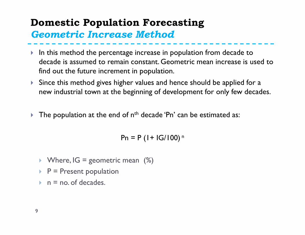
� In this method the percentage increase in population from decade to decade is assumed to remain constant. Geometric mean increase is used to find out the future increment in population.

� Since this method gives higher values and hence should be applied for a new industrial town at the beginning of development for only few decades.

� The population at the end of nth decade ‘Pn’ can be estimated as:

Pn = P (1+ IG/100) n

� Where, IG = geometric mean (%)

� P = Present population

� n = no. of decades.


Incremental Increase Method

10

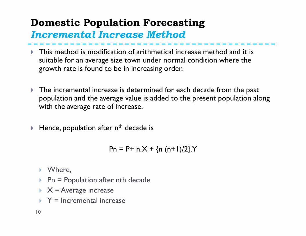
� This method is modification of arithmetical increase method and it is suitable for an average size town under normal condition where the growth rate is found to be in increasing order.

� The incremental increase is determined for each decade from the past population and the average value is added to the present population along with the average rate of increase.

� Hence, population after nth decade is

Pn = P+ n.X + {n (n+1)/2}.Y

� Where,

� Pn = Population after nth decade

� X = Average increase

� Y = Incremental increase


Graphical Method

11

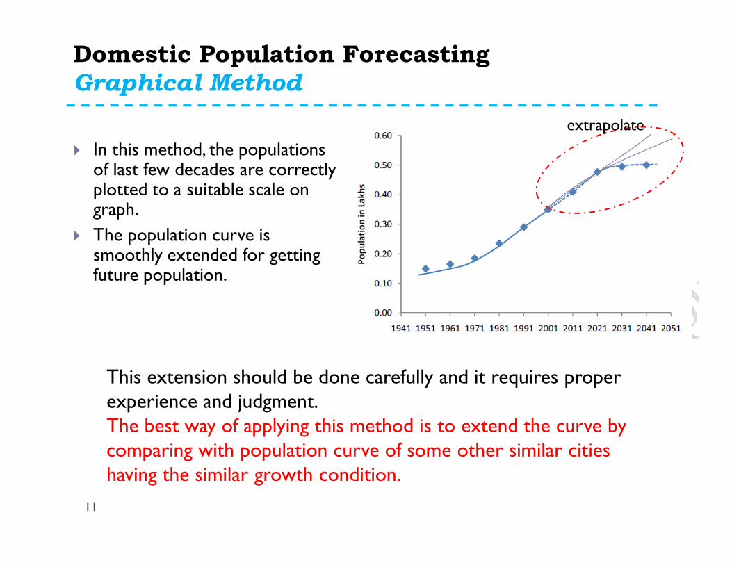
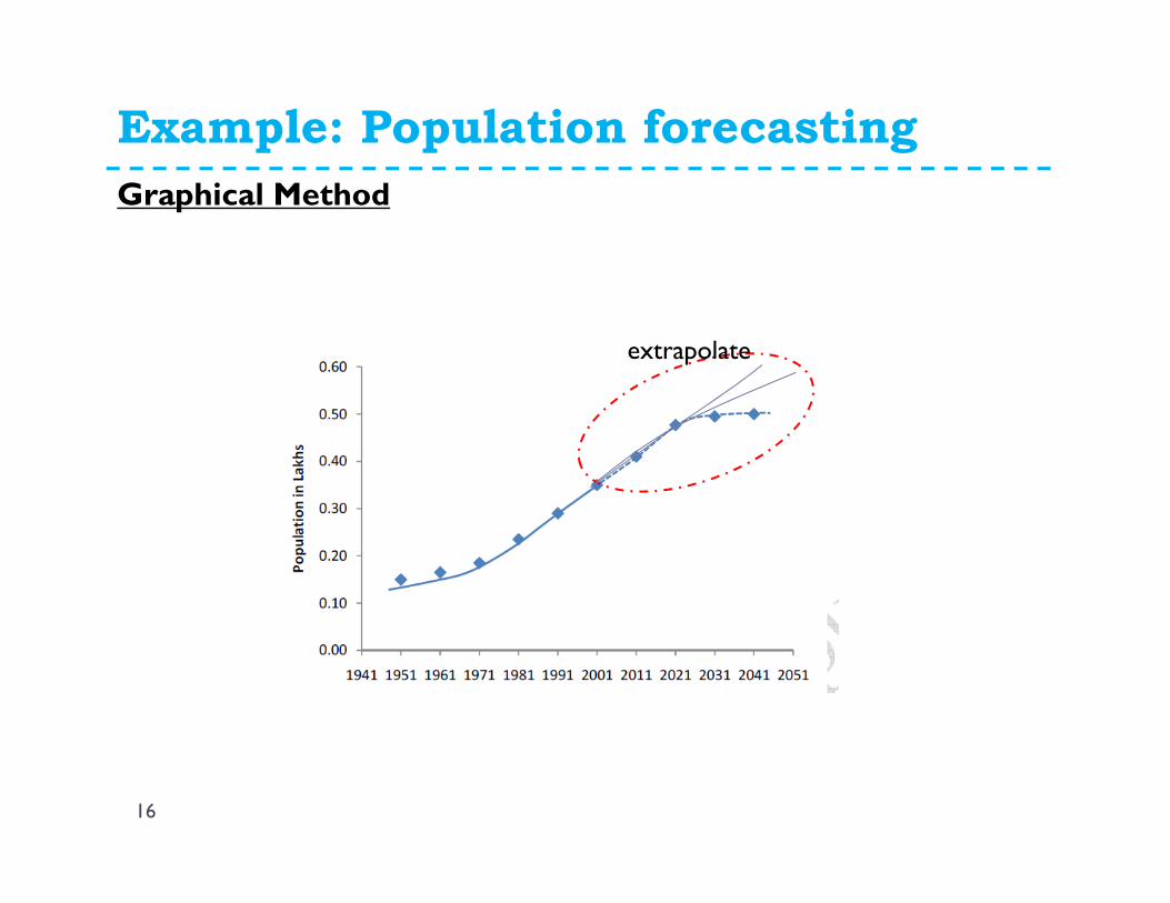
� In this method, the populations of last few decades are correctly plotted to a suitable scale on graph.

� The population curve is smoothly extended for getting future population.

This extension should be done carefully and it requires proper experience and judgment. The best way of applying this method is to extend the curve by comparing with population curve of some other similar cities having the similar growth condition.

extrapolate

Example: Population forecasting

12

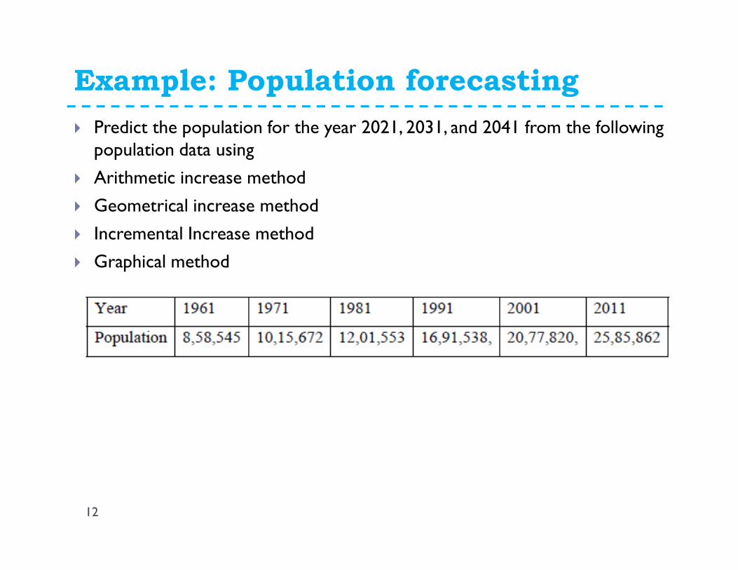
� Predict the population for the year 2021, 2031, and 2041 from the following population data using

� Arithmetic increase method

� Geometrical increase method

� Incremental Increase method

� Graphical method


13

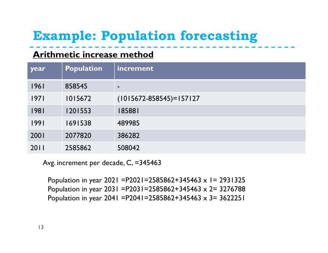
year Population increment

1961 858545 -

1971 1015672 (1015672-858545)=157127

1981 1201553 185881

1991 1691538 489985

2001 2077820 386282

2011 2585862 508042

Arithmetic increase method

Avg. increment per decade, C, =345463

Population in year 2021 =P2021=2585862+345463 x 1= 2931325Population in year 2031 =P2031=2585862+345463 x 2= 3276788Population in year 2041 =P2041=2585862+345463 x 3= 3622251


14

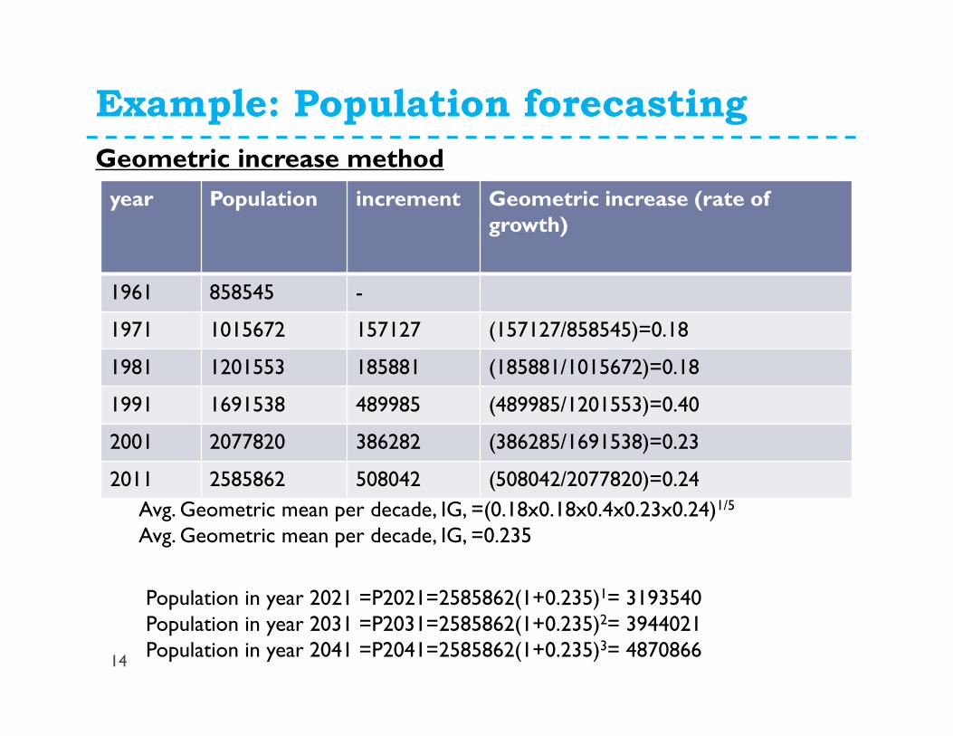
year Population increment Geometric increase (rate of growth)

1961 858545 -

1971 1015672 157127 (157127/858545)=0.18

1981 1201553 185881 (185881/1015672)=0.18

1991 1691538 489985 (489985/1201553)=0.40

2001 2077820 386282 (386285/1691538)=0.23

2011 2585862 508042 (508042/2077820)=0.24

Geometric increase method

Avg. Geometric mean per decade, IG, =(0.18x0.18x0.4x0.23x0.24)1/5

Avg. Geometric mean per decade, IG, =0.235

Population in year 2021 =P2021=2585862(1+0.235)1= 3193540Population in year 2031 =P2031=2585862(1+0.235)2= 3944021Population in year 2041 =P2041=2585862(1+0.235)3= 4870866


15

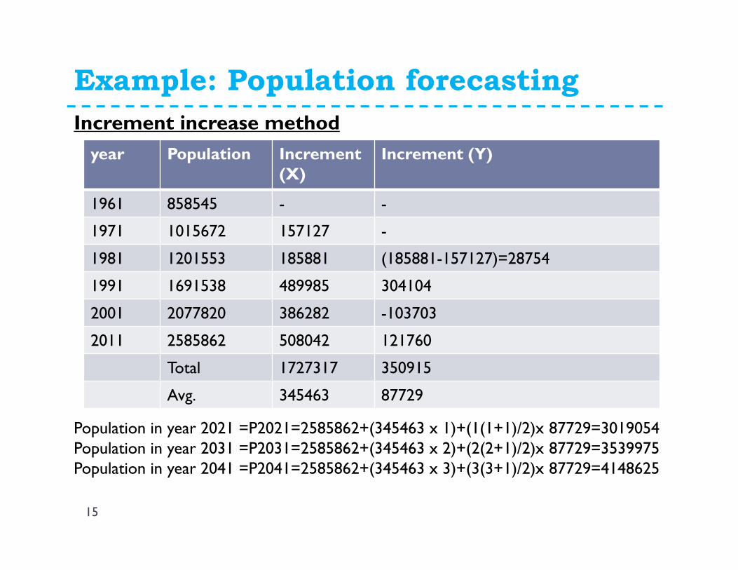
year Population Increment (X)

Increment (Y)

1961 858545 - -

1971 1015672 157127 -

1981 1201553 185881 (185881-157127)=28754

1991 1691538 489985 304104

2001 2077820 386282 -103703

2011 2585862 508042 121760

Total 1727317 350915

Avg. 345463 87729

Increment increase method

Population in year 2021 =P2021=2585862+(345463 x 1)+(1(1+1)/2)x 87729=3019054Population in year 2031 =P2031=2585862+(345463 x 2)+(2(2+1)/2)x 87729=3539975Population in year 2041 =P2041=2585862+(345463 x 3)+(3(3+1)/2)x 87729=4148625


16

Graphical Method

extrapolate


Comparative Graphical Method

17

� In this method the census populations of cities already developed under similar conditions are plotted.

� The curve of past population of the city under consideration is plotted on the same graph.

� The curve is extended carefully by comparing with the population curve of some similar cities having the similar condition of growth.

� The advantage of this method is that the future population can be predicted from the present population even in the absent of some of the past census report.



18

� Example: Let the population of a new city X be given for decades 1970, 1980, 1990 and 2000 were 32,000; 38,000; 43,000 and 50,000, respectively. The cities A, B, C and D were developed in similar conditions as that of city X. It is required to estimate the population of the city X in the years 2010 and 2020.

� The population of cities A, B, C and D of different decades were given below:

� (i) City A was 50,000; 62,000; 72,000 and 87,000 in 1960, 1972, 1980 and 1990, respectively.

� (ii) City B was 50,000; 58,000; 69,000 and 76,000 in 1962, 1970, 1981 and 1988, respectively.

� (iii) City C was 50,000; 56,500; 64,000 and 70,000 in 1964, 1970, 1980 and 1988, respectively.

� (iv) City D was 50,000; 54,000; 58,000 and 62,000 in 1961, 1973, 1982 and 1989, respectively.



19

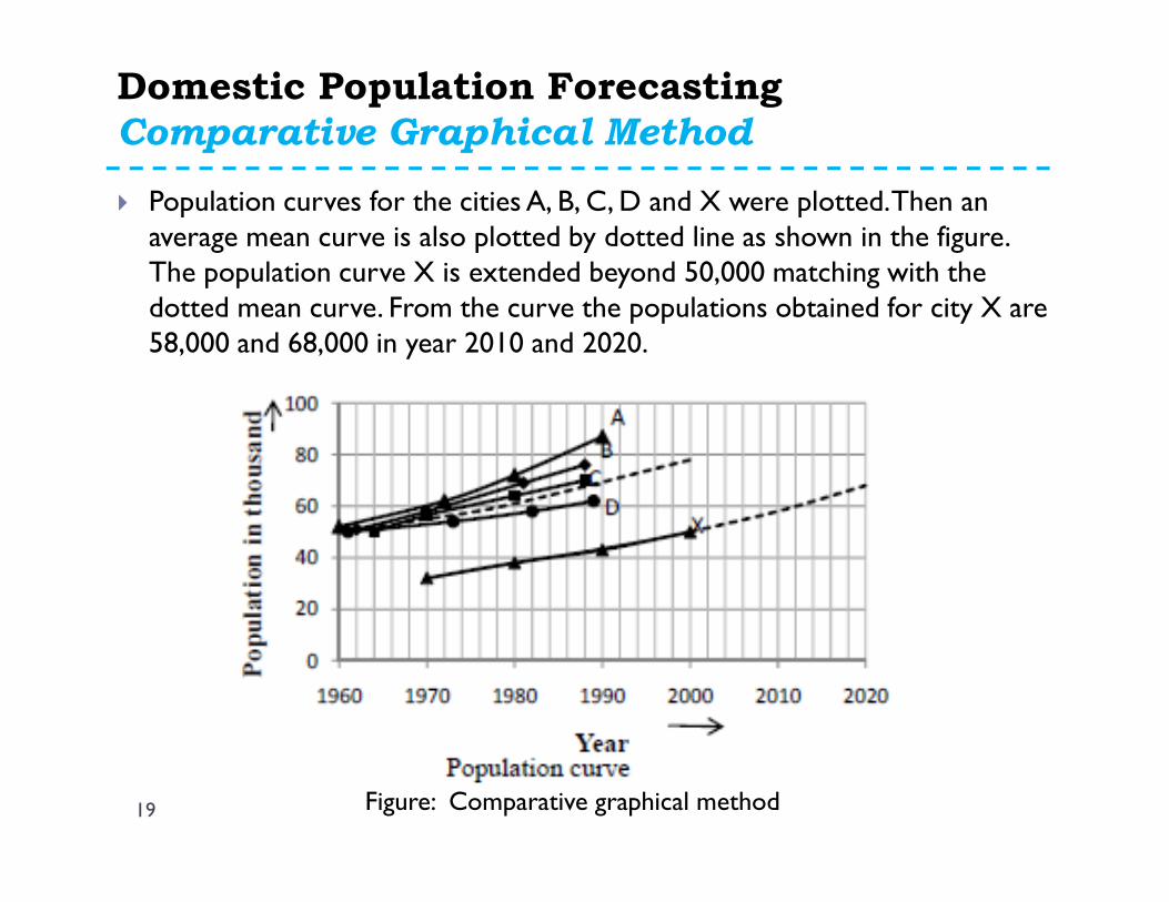
� Population curves for the cities A, B, C, D and X were plotted. Then an average mean curve is also plotted by dotted line as shown in the figure. The population curve X is extended beyond 50,000 matching with the dotted mean curve. From the curve the populations obtained for city X are 58,000 and 68,000 in year 2010 and 2020.

Figure: Comparative graphical method


Master Plan Method

20

� The big and metropolitan cities are generally not developed in haphazard manner, but are planned and regulated by local bodies according to master plan.

� The master plan is prepared for next 25 to 30 years for the city.

� According to the master plan the city is divided into various zones such as residence, commerce and industry.

� The population densities are fixed for various zones in the master plan.

� From this population density total water demand and wastewater generation for that zone can be worked out. So by this method it is very easy to access precisely the design population.

Domestic Population ForecastingRatio Method

21

� In this method, the local population and the country's population for the last four to five decades is obtained from the census records.

� The ratios of the local population to national population are then worked out for these decades.

� A graph is then plotted between time and these ratios, and extended up to the design period to extrapolate the ratio corresponding to future design year.

� This ratio is then multiplied by the expected national population at the end of the design period, so as to obtain the required city's future population.Drawbacks:

� Depends on accuracy of national population estimate.

� Does not consider the abnormal or special conditions which can lead to population shifts from one city to another.

Domestic Population Forecasting Logistic Curve Method

22

� This method is used when the growth rate of population due to births, deaths and migrations takes place under normal situation and it is not subjected to any extraordinary changes like epidemic, war, earth quake or any natural disaster etc.

� The population follows the growth curve characteristics of living things within limited space and economic opportunity.

� If the population of a city is plotted with respect to time, the curve so obtained under normal condition will look like S-shaped curve and is known as logistic curve.


Logistic Curve Method

23

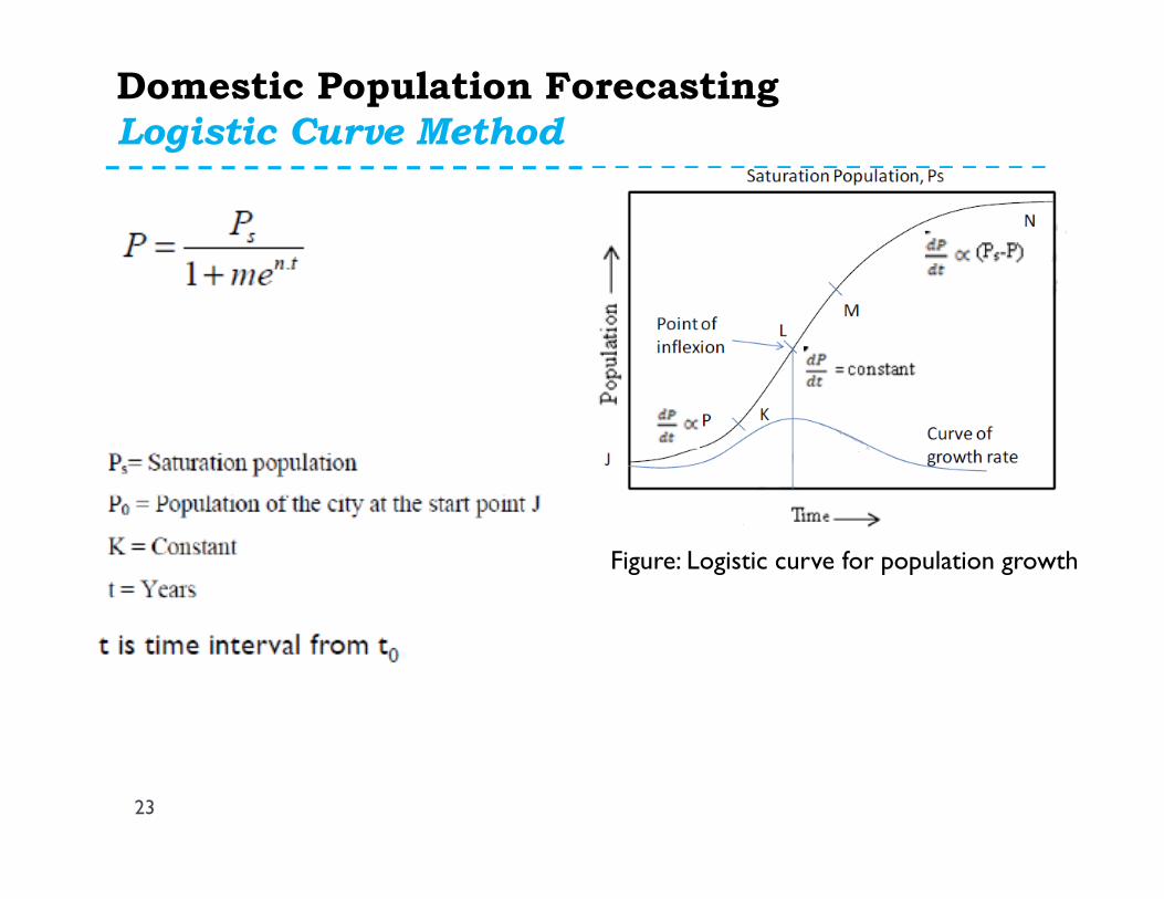
Figure: Logistic curve for population growth



24

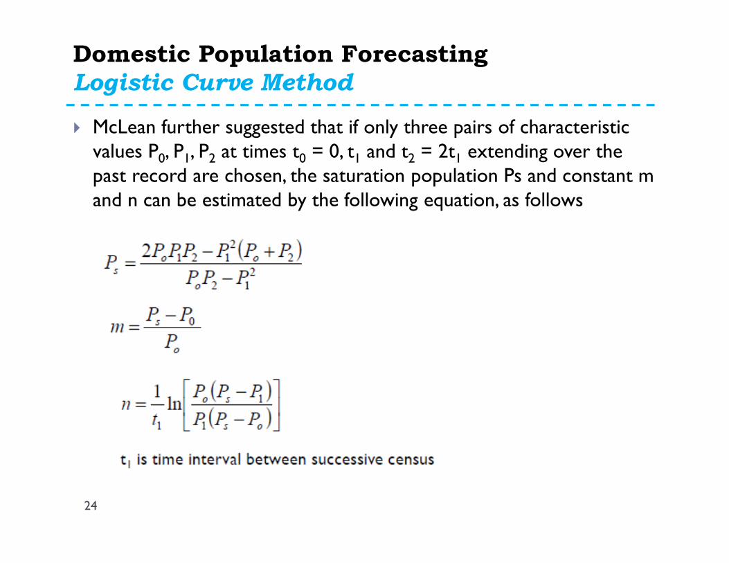
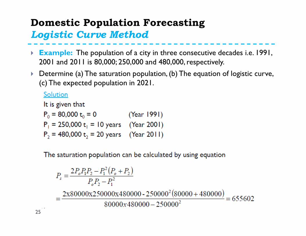
� McLean further suggested that if only three pairs of characteristic values P0, P1, P2 at times t0 = 0, t1 and t2 = 2t1 extending over the past record are chosen, the saturation population Ps and constant m and n can be estimated by the following equation, as follows



25

� Example: The population of a city in three consecutive decades i.e. 1991, 2001 and 2011 is 80,000; 250,000 and 480,000, respectively.

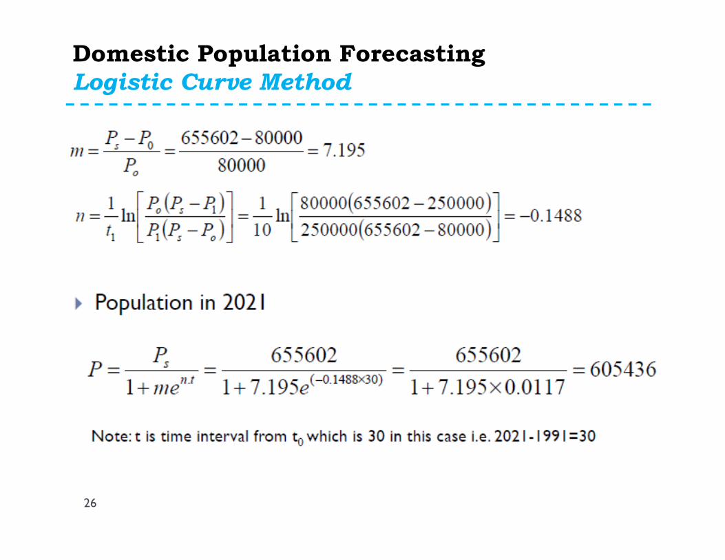
� Determine (a) The saturation population, (b) The equation of logistic curve, (c) The expected population in 2021.



26

Home Exercise

27

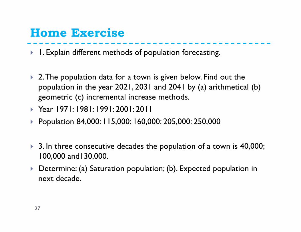
� 1. Explain different methods of population forecasting.

� 2. The population data for a town is given below. Find out the population in the year 2021, 2031 and 2041 by (a) arithmetical (b) geometric (c) incremental increase methods.

� Year 1971: 1981: 1991: 2001: 2011

� Population 84,000: 115,000: 160,000: 205,000: 250,000

� 3. In three consecutive decades the population of a town is 40,000; 100,000 and130,000.

� Determine: (a) Saturation population; (b). Expected population in next decade.

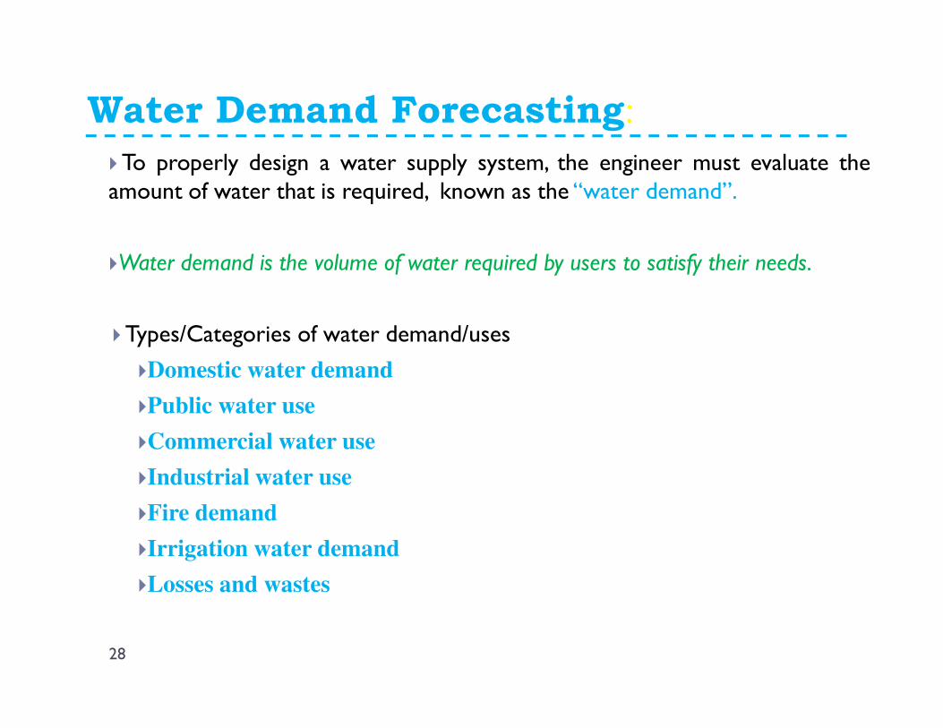
�To properly design a water supply system, the engineer must evaluate theamount of water that is required, known as the “water demand”.

�Water demand is the volume of water required by users to satisfy their needs.

�Types/Categories of water demand/uses

�Domestic water demand

�Public water use

�Commercial water use

�Industrial water use

�Fire demand

�Irrigation water demand

�Losses and wastes

Water Demand Forecasting:

28

Typical Water Demands

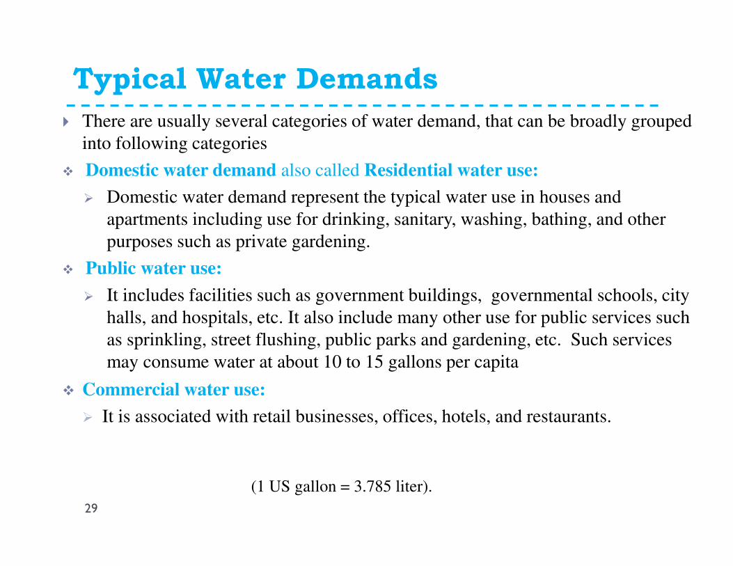
� There are usually several categories of water demand, that can be broadly grouped

into following categories

� Domestic water demand also called Residential water use:

� Domestic water demand represent the typical water use in houses and

apartments including use for drinking, sanitary, washing, bathing, and other

purposes such as private gardening.

� Public water use:

� It includes facilities such as government buildings, governmental schools, city

halls, and hospitals, etc. It also include many other use for public services such

as sprinkling, street flushing, public parks and gardening, etc. Such services

may consume water at about 10 to 15 gallons per capita

� Commercial water use:

� It is associated with retail businesses, offices, hotels, and restaurants.

(1 US gallon = 3.785 liter).

29


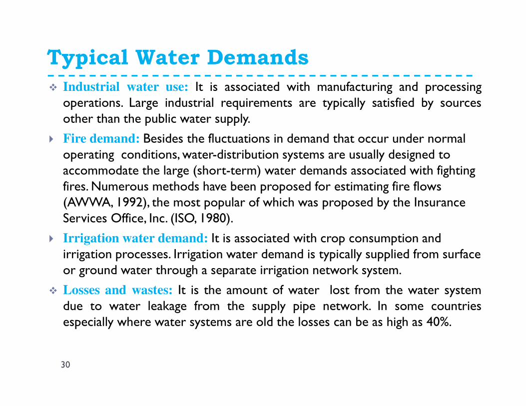
� Industrial water use: It is associated with manufacturing and processingoperations. Large industrial requirements are typically satisfied by sourcesother than the public water supply.

� Fire demand: Besides the fluctuations in demand that occur under normal operating conditions, water-distribution systems are usually designed to accommodate the large (short-term) water demands associated with fighting fires. Numerous methods have been proposed for estimating fire flows (AWWA, 1992), the most popular of which was proposed by the Insurance Services Office, Inc. (ISO, 1980).

� Irrigation water demand: It is associated with crop consumption and irrigation processes. Irrigation water demand is typically supplied from surface or ground water through a separate irrigation network system.

� Losses and wastes: It is the amount of water lost from the water systemdue to water leakage from the supply pipe network. In some countriesespecially where water systems are old the losses can be as high as 40%.

30


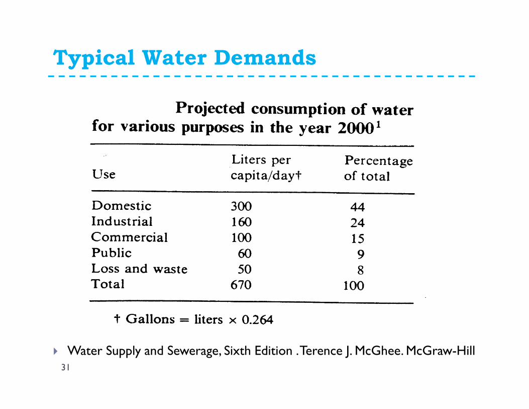
31

� Water Supply and Sewerage, Sixth Edition . Terence J. McGhee. McGraw-Hill


32

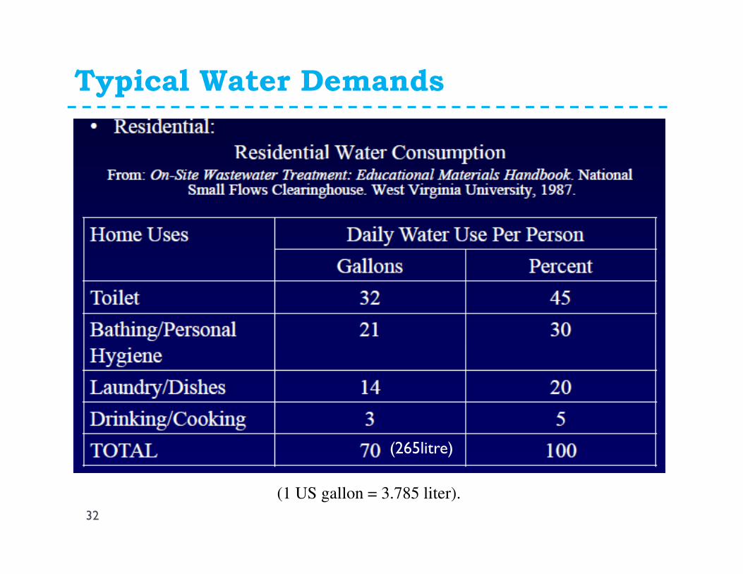
(1 US gallon = 3.785 liter).

(265litre)

FACTORS AFFECTING WATER CONSUMPTION

� Climate conditions: Warm dry regions have higher consumption rates thancooler regions. In addition, water usage is affected by the precipitation levelsin the region.

� Size of the city. In small cities, it was found that the per capita per day waterconsumption was small due to the fact that there are only limited uses ofwater in those cities. Small cities have larger area that is inadequately servedby both water and sewer systems than larger cities.

� Characteristics of the population. Domestic use of water was found tovary widely. This is largely dependent upon the economic status of theconsumers, which will differ greatly in various sections of a city. In high-value residential areas of a city the water consumption per capita will be highand vice versa

33

� Metering. Communities that are metered usually show a lower and morestable water use pattern.

� Water quality. Consumer perception of bad water quality can decrease thewater usage rate.

� Cost of water. A tendency toward water conservation occur when cost ofwater is high.

� Water pressure. Rates of water usage increase with increases in waterpressure.

� Water conservation. Public awareness and implementation of waterconservation programs by utilities tend to have an impact on the water usagerate.

FACTORS AFFECTING WATER CONSUMPTION

34

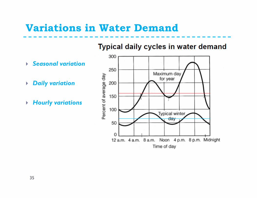
Variations in Water Demand

35

� Seasonal variation

� Daily variation

� Hourly variations

Water Demands: Terminologies

36

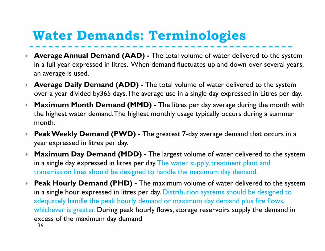
� Average Annual Demand (AAD) - The total volume of water delivered to the system in a full year expressed in litres. When demand fluctuates up and down over several years, an average is used.

� Average Daily Demand (ADD) - The total volume of water delivered to the system over a year divided by365 days. The average use in a single day expressed in Litres per day.

� Maximum Month Demand (MMD) - The litres per day average during the month with the highest water demand. The highest monthly usage typically occurs during a summer month.

� Peak Weekly Demand (PWD) - The greatest 7-day average demand that occurs in a year expressed in litres per day.

� Maximum Day Demand (MDD) - The largest volume of water delivered to the system in a single day expressed in litres per day. The water supply, treatment plant and transmission lines should be designed to handle the maximum day demand.

� Peak Hourly Demand (PHD) - The maximum volume of water delivered to the system in a single hour expressed in litres per day. Distribution systems should be designed to adequately handle the peak hourly demand or maximum day demand plus fire flows, whichever is greater. During peak hourly flows, storage reservoirs supply the demand in excess of the maximum day demand

Peak Water Use Estimation: Estimation of

Average Daily Rate Based on a Maximum Time Period

37

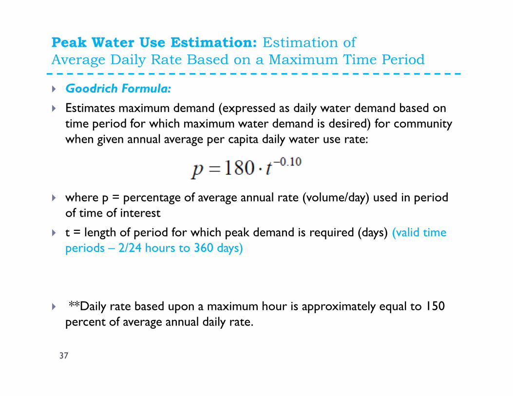
� Goodrich Formula:

� Estimates maximum demand (expressed as daily water demand based on time period for which maximum water demand is desired) for community when given annual average per capita daily water use rate:

� where p = percentage of average annual rate (volume/day) used in period of time of interest

� t = length of period for which peak demand is required (days) (valid time periods – 2/24 hours to 360 days)

� **Daily rate based upon a maximum hour is approximately equal to 150 percent of average annual daily rate.

Peak Water Use Estimation

38

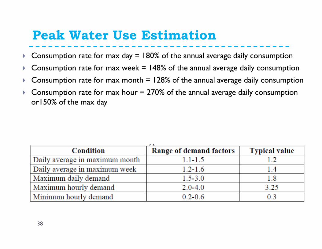
� Consumption rate for max day = 180% of the annual average daily consumption

� Consumption rate for max week = 148% of the annual average daily consumption

� Consumption rate for max month = 128% of the annual average daily consumption

� Consumption rate for max hour = 270% of the annual average daily consumption or150% of the max day

Example

39

� Estimate average and maximum daily demand/flow for a community with a population of 22000 having an average consumption of 600litre/capita/day

Fire Demand

40

� Fire flow is defined as the rate of water flow needed to control a fire (AWWA, 2008).

� Adequate fire flow is critical for the effective extinguishing of a fire.

� If the fire flow is over calculated, there could be a negative impact on the water distribution systems. If the fire flow is under calculated, a fire may result in the loss of the building of lives.

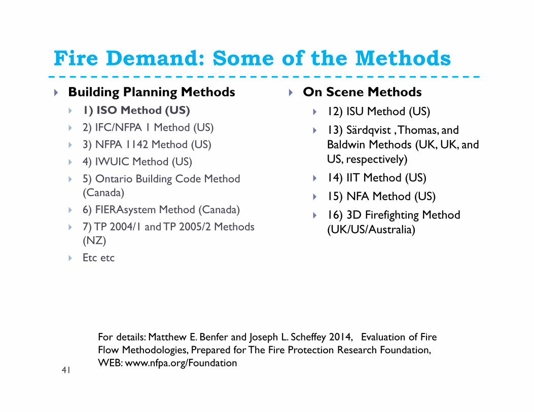
Fire Demand: Some of the Methods

41

� Building Planning Methods

� 1) ISO Method (US)

� 2) IFC/NFPA 1 Method (US)

� 3) NFPA 1142 Method (US)

� 4) IWUIC Method (US)

� 5) Ontario Building Code Method (Canada)

� 6) FIERAsystem Method (Canada)

� 7) TP 2004/1 and TP 2005/2 Methods (NZ)

� Etc etc

� On Scene Methods

� 12) ISU Method (US)

� 13) Särdqvist , Thomas, and Baldwin Methods (UK, UK, and US, respectively)

� 14) IIT Method (US)

� 15) NFA Method (US)

� 16) 3D Firefighting Method (UK/US/Australia)

For details: Matthew E. Benfer and Joseph L. Scheffey 2014, Evaluation of Fire Flow Methodologies, Prepared for The Fire Protection Research Foundation, WEB: www.nfpa.org/Foundation

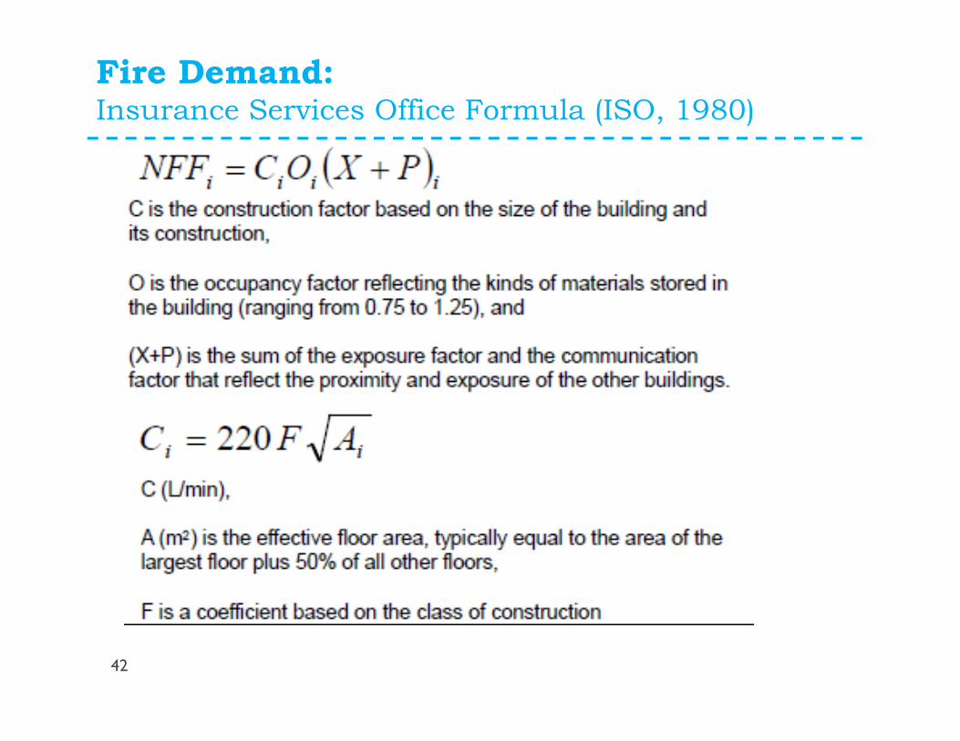
Fire Demand: Insurance Services Office Formula (ISO, 1980)

42

Fire Demand

43

� Maximum and Minimum Value of C:

� The value of C shall not exceed

� 8,000 gpm (32000L/min) for Construction Class 1 and 2

� 6,000 gpm (24000L/min) for Construction Class 3, 4, 5, and 6

� 6,000 gpm (24000L/min) for a 1-story building of any class of construction

� The value of C shall not be less than 500 gpm (2000L/min).

� ISO rounds the calculated value of C to the nearest 250 gpm (1000L/min).

1gallon=3.79liter~4Liters

Fire Demand

44

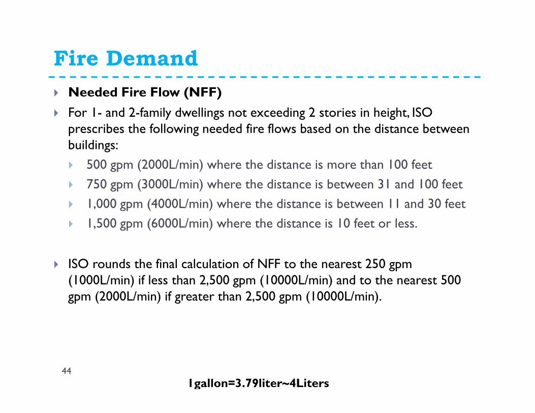
� Needed Fire Flow (NFF)

� For 1- and 2-family dwellings not exceeding 2 stories in height, ISO prescribes the following needed fire flows based on the distance between buildings:

� 500 gpm (2000L/min) where the distance is more than 100 feet

� 750 gpm (3000L/min) where the distance is between 31 and 100 feet

� 1,000 gpm (4000L/min) where the distance is between 11 and 30 feet

� 1,500 gpm (6000L/min) where the distance is 10 feet or less.

� ISO rounds the final calculation of NFF to the nearest 250 gpm(1000L/min) if less than 2,500 gpm (10000L/min) and to the nearest 500 gpm (2000L/min) if greater than 2,500 gpm (10000L/min).

1gallon=3.79liter~4Liters

Fire Demand

45

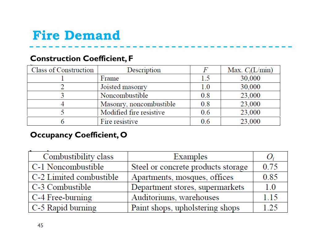
Construction Coefficient, F

Occupancy Coefficient, O

Fire Demand

46

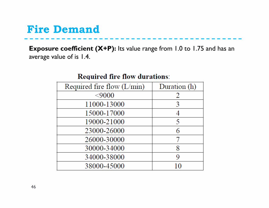
Exposure coefficient (X+P): Its value range from 1.0 to 1.75 and has an average value of is 1.4.

Fire Demand

47

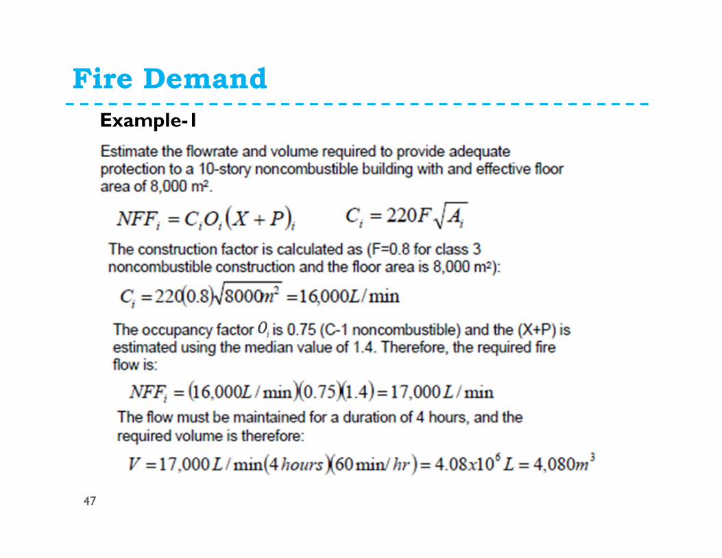
Example-1

Fire Demand

48

� Example-2: Estimate the flowrate and volume required to provide adequate protection to 20 story non-combustible building. Let each floor has an area of 1000m2.

� The construction factor is calculated as F=0.8 for class 3 non-combustible construction.

� Floor area of building=Ai=1000+0.5(1000)x19=10500m2

Ci=220(0.8)(10500)0.5=16395L/min

� The occupancy factor is 0.75 (C-1 non-combustible) and the (X+P) is estimated using the median value of 1.4. Therefore the required fire flow is

NFFi=Ci Oi (X+P) i=16395(0.75)(1.4)=17214=18000L/min

� If the flow must be maintained for a duration of 4 hours, the total required volume will be

=18000(4x60)= 4320000L=4320m3

Fire Demand: Fire Hydrants

49

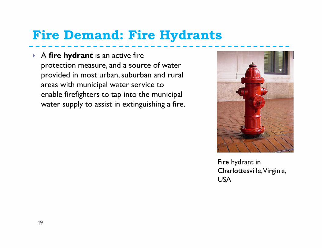
� A fire hydrant is an active fire protection measure, and a source of water provided in most urban, suburban and rural areas with municipal water service to enable firefighters to tap into the municipal water supply to assist in extinguishing a fire.

Fire hydrant in Charlottesville, Virginia, USA

Fire Demand: Fire Hydrants Spacing and

Discharge

50

� Guidelines are not uniformly defined and varies wide according to municipality. Typical information on spacing and discharge are given below;

� Capacity of a fire hydrant is 30 m3/h (500L/min) to 60 m3/h (1000L/min) and should be within 40m (130ft) to 50m(165ft) from every object. This results in fire hydrants every 80m (262ft) to 100m (328ft) in a distribution network.

� Looking at single- family houses with an average width of 4 (13ft) to 5 (16ft) meters, this means that for every 20 to 25 houses a fire hydrant is needed.

� Required fire flows, plus domestic demand, must be available within the water system at a minimum of 20 psi (150kPa) residual pressure.

� For details refer to guideline of fire hydrant spacing & fire flow requirements issued by municipality

Design Flows

� The required capacities consist of various combinations of

� the maximum daily demand,

� maximum hourly demand,

� and the fire demand.

� Typically, the delivery pipelines from the water source to the treatment plant, as well as the treatment plant itself, are designed with a capacity equal to the maximum daily demand.

� The flow rates and pressures in the distribution system are analyzed under both maximum daily plus fire demand and the maximum hourly demand, and the larger flow rate governs the design.

� Pumps are sized for a variety of conditions from maximum daily to maximum hourly demand, depending on their function in the distribution system.

� Additional reserve capacity is usually installed in water-supply systems to allow for redundancy and maintenance requirements.

51

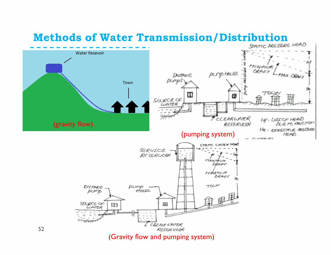
Methods of Water Transmission/Distribution

52

� (pumping system)

(gravity flow)

(pumping system)

(Gravity flow and pumping system)

Methods of Water Distribution

53

� Gravity flow and pumping with storage (Pumping with Storage)

� Most common

� Water supplied at approximately uniform rate

� Flow in excess of consumption stored in elevated tanks

� Tank water provides flow and pressure when use is high

� Fire-fighting

� High-use hours

� Flow during power failure

Water Distribution System Components

54

� Pumping Stations

� Distribution Storage (reservoirs or tanks)

� Distribution System Piping (transmission system)

� Other water system components include water source and water treatment

Distribution Reservoirs/Tanks

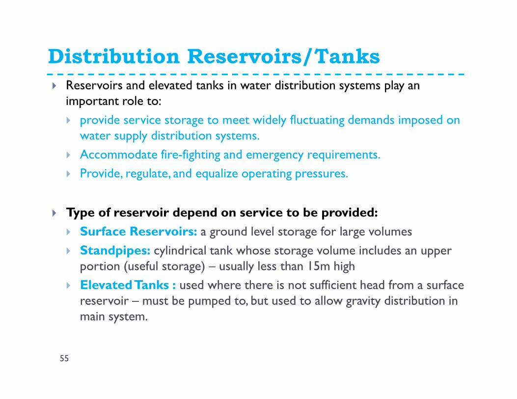
� Reservoirs and elevated tanks in water distribution systems play an important role to:

� provide service storage to meet widely fluctuating demands imposed on water supply distribution systems.

� Accommodate fire-fighting and emergency requirements.

� Provide, regulate, and equalize operating pressures.

� Type of reservoir depend on service to be provided:

� Surface Reservoirs: a ground level storage for large volumes

� Standpipes: cylindrical tank whose storage volume includes an upper portion (useful storage) – usually less than 15m high

� Elevated Tanks : used where there is not sufficient head from a surface reservoir – must be pumped to, but used to allow gravity distribution in main system.

55

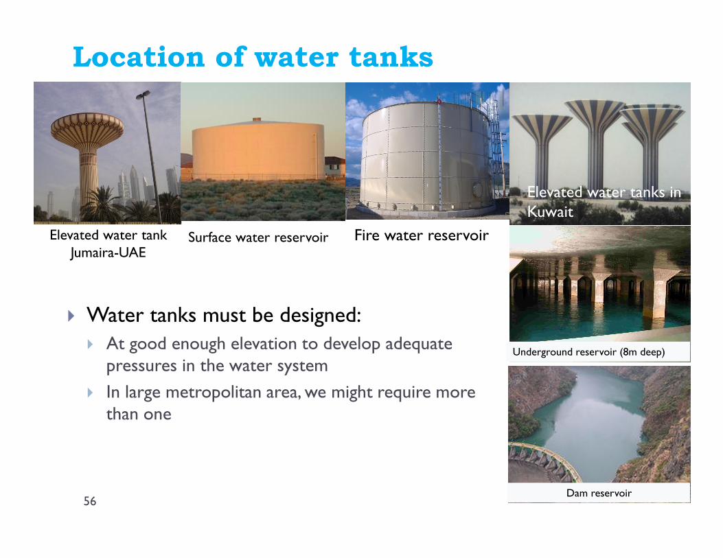
Location of water tanks

Fire water reservoirElevated water tank Jumaira-UAE

Surface water reservoir

Elevated water tanks in Kuwait

Underground reservoir (8m deep)

Dam reservoir

� Water tanks must be designed:

� At good enough elevation to develop adequate pressures in the water system

� In large metropolitan area, we might require more than one

56

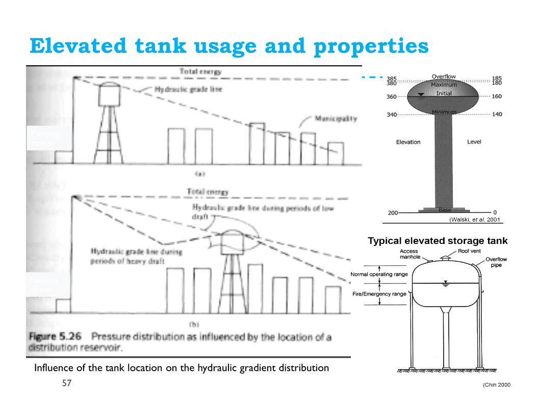
Elevated tank usage and properties

Influence of the tank location on the hydraulic gradient distribution

Pumping station

Pumping station

57

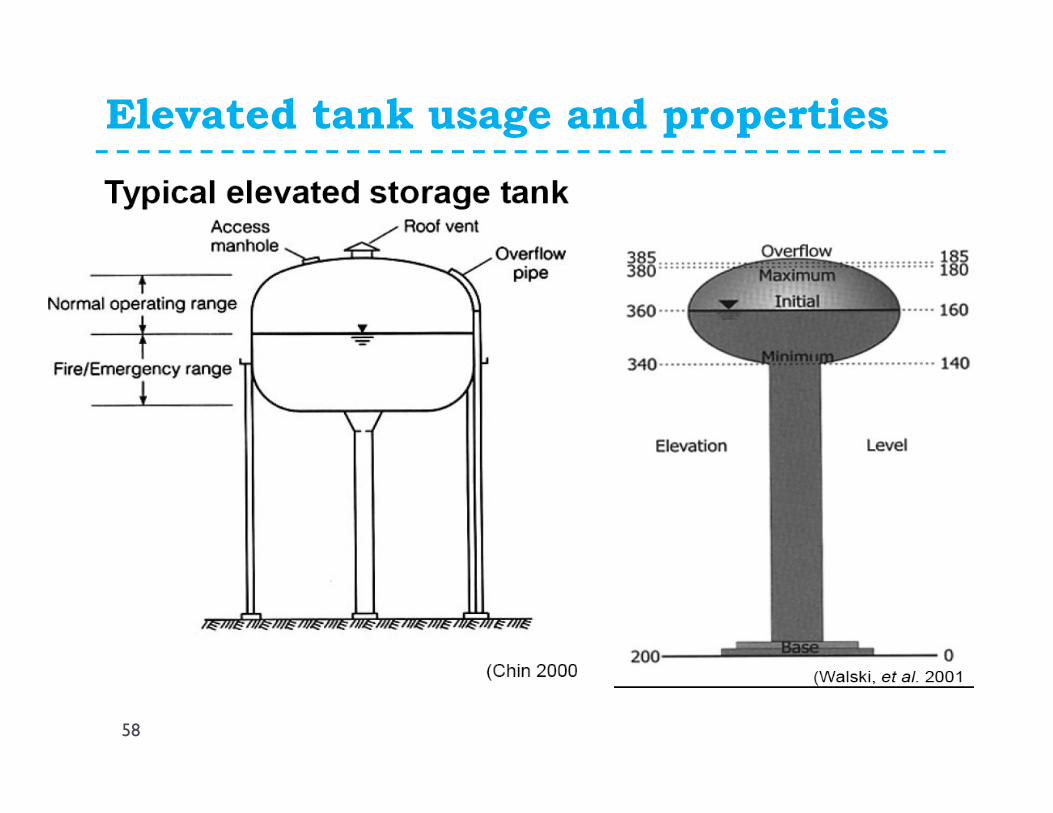
Elevated tank usage and properties

58

Storage Design Criteria

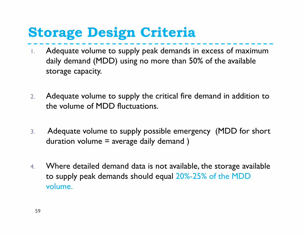
1. Adequate volume to supply peak demands in excess of maximum daily demand (MDD) using no more than 50% of the available storage capacity.

2. Adequate volume to supply the critical fire demand in addition to the volume of MDD fluctuations.

3. Adequate volume to supply possible emergency (MDD for short duration volume = average daily demand )

4. Where detailed demand data is not available, the storage available to supply peak demands should equal 20%-25% of the MDD volume.

59

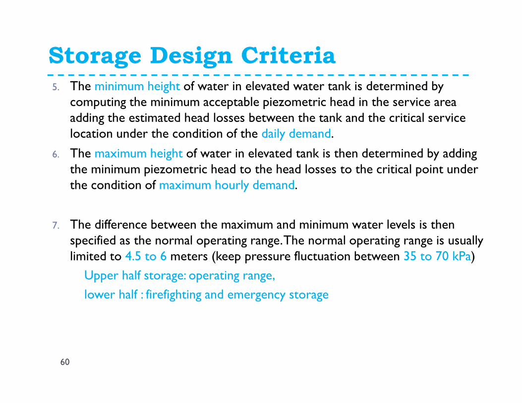
Storage Design Criteria5. The minimum height of water in elevated water tank is determined by

computing the minimum acceptable piezometric head in the service area adding the estimated head losses between the tank and the critical service location under the condition of the daily demand.

6. The maximum height of water in elevated tank is then determined by adding the minimum piezometric head to the head losses to the critical point under the condition of maximum hourly demand.

7. The difference between the maximum and minimum water levels is then specified as the normal operating range. The normal operating range is usually limited to 4.5 to 6 meters (keep pressure fluctuation between 35 to 70 kPa)

Upper half storage: operating range,

lower half : firefighting and emergency storage

60

Example

61

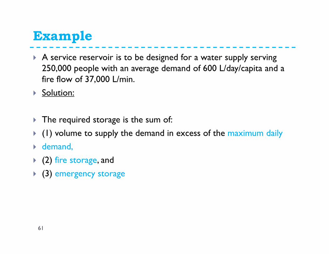
� A service reservoir is to be designed for a water supply serving 250,000 people with an average demand of 600 L/day/capita and a fire flow of 37,000 L/min.

� Solution:

� The required storage is the sum of:

� (1) volume to supply the demand in excess of the maximum daily

� demand,

� (2) fire storage, and

� (3) emergency storage

Example

62

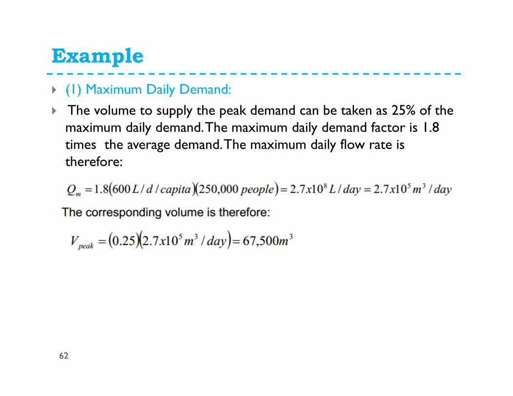
� (1) Maximum Daily Demand:

� The volume to supply the peak demand can be taken as 25% of the maximum daily demand. The maximum daily demand factor is 1.8 times the average demand. The maximum daily flow rate is therefore:

Example

63

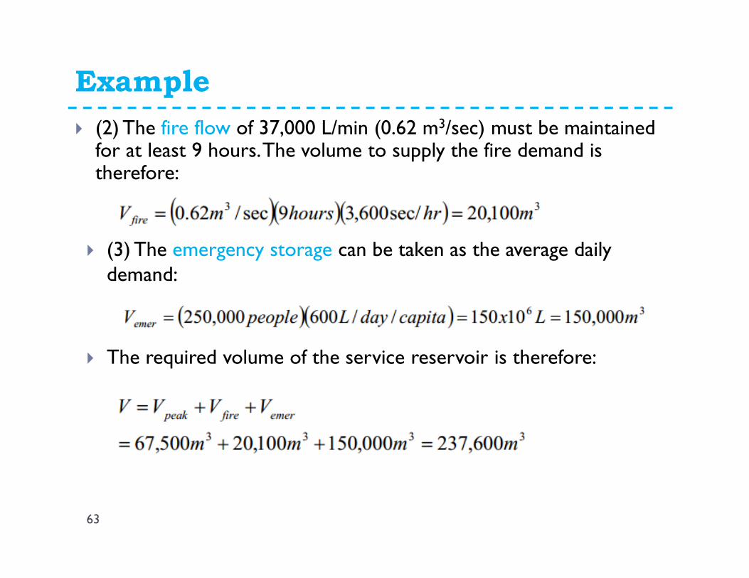
� (2) The fire flow of 37,000 L/min (0.62 m3/sec) must be maintained for at least 9 hours. The volume to supply the fire demand is therefore:

� (3) The emergency storage can be taken as the average daily demand:

� The required volume of the service reservoir is therefore:

Example

64

� A service reservoir is to be designed for a water supply serving 100,000 people with an average demand of 600 L/day/capita and a fire flow of 17,000 L/min.

� Solve

Example

65

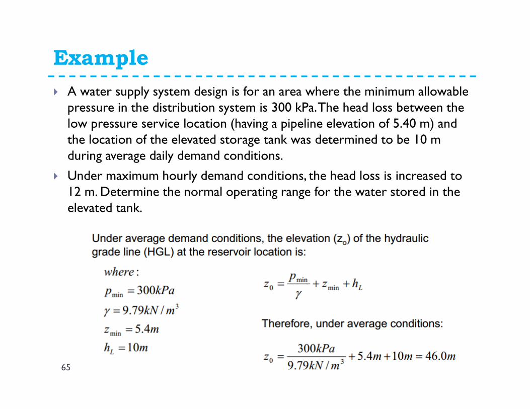
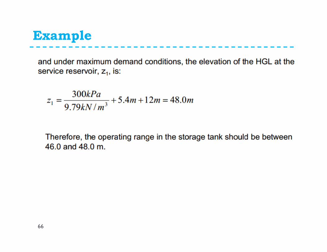
� A water supply system design is for an area where the minimum allowable pressure in the distribution system is 300 kPa. The head loss between the low pressure service location (having a pipeline elevation of 5.40 m) and the location of the elevated storage tank was determined to be 10 m during average daily demand conditions.

� Under maximum hourly demand conditions, the head loss is increased to 12 m. Determine the normal operating range for the water stored in the elevated tank.

Example

66

Water Transmission(Distribution System Piping)

67

� Water transmission refers to the transportation of the water from the source to the treatment plant and to the area of distribution.

� It can be realized through

� free-flow conduits,

� pressurized pipelines or

� a combination of the two.

� For small community water supplies pressurized pipelined (e.g., piping system) are most common, since they are not very limited by the topography of the area to be traversed.

� Free-flow conduits (e.g., canals, aqueducts and tunnels) are preferred in hilly areas or in areas where the required slope of the conduit more or less coincides with the slope of the terrain.

The Pipe System

68

� Primary mains

� Secondary lines

� Small distribution lines

� Primary Mains (Arterial Mains)

� Form the basic structure of the system and carry flow from the pumping station to elevated storage tanks and from elevated storage tanks to the various districts of the city

� Laid out in interlocking loops

� Mains not more than 1 km (3000 ft) apart

� Valved at intervals of not more than 1.5 km (1 mile)

� Smaller lines connecting to them are valved

The Pipe System

69

� Secondary Lines

� Form smaller loops within the primary main system

� Run from one primary line to another

� Spacing of 2 to 4 blocks

� Provide large amounts of water for fire fighting with out excessive pressure loss

� Small distribution lines

� Form a grid over the entire service area

� Supply water to every user and fire hydrants

� Connected to primary, secondary, or other small mains at both ends

� Valved so the system can be shut down for repairs

� Size may be dictated by fire flow except in residential areas with very large lots

Pipe Sizes in Municipal Distribution Systems

70

� Small distribution lines providing only domestic flow may be as small as 100mm (4in) but,

� <1300 ft in length if dead ended or

� <2000 ft if connected to system at both ends

� Otherwise small distribution mains > 150mm (6in)

� High value districts-minimum mains > 200mm (8 in)

� Major streets - minimum size 300mm (12 in)

� Fire fighting requirement >150mm (6 inch)

� National Board of Fire Underwrites > 200mm (8inch)

Velocity in Municipal Distribution Systems

71

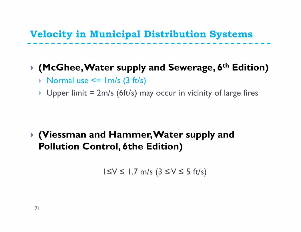
� (McGhee, Water supply and Sewerage, 6th Edition)

� Normal use <= 1m/s (3 ft/s)

� Upper limit = 2m/s (6ft/s) may occur in vicinity of large fires

� (Viessman and Hammer, Water supply and Pollution Control, 6the Edition)

1≤V ≤ 1.7 m/s (3 ≤ V ≤ 5 ft/s)

Pressure in Municipal Distribution System

72

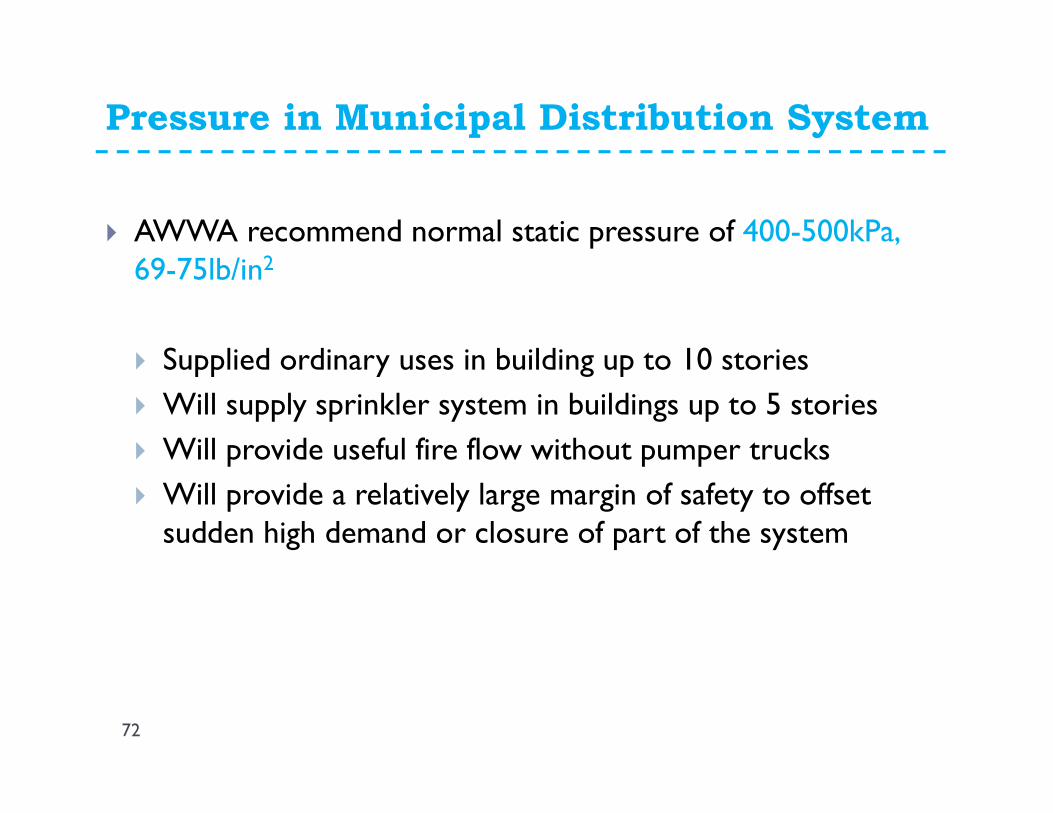
� AWWA recommend normal static pressure of 400-500kPa, 69-75lb/in2

� Supplied ordinary uses in building up to 10 stories

� Will supply sprinkler system in buildings up to 5 stories

� Will provide useful fire flow without pumper trucks

� Will provide a relatively large margin of safety to offset sudden high demand or closure of part of the system

Pressure in Municipal Distribution Systems

73

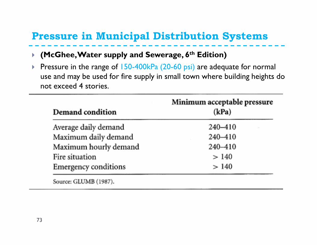
� (McGhee, Water supply and Sewerage, 6th Edition)

� Pressure in the range of 150-400kPa (20-60 psi) are adequate for normal use and may be used for fire supply in small town where building heights do not exceed 4 stories.

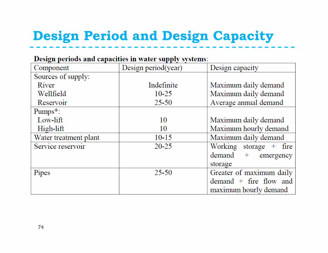
Design Period and Design Capacity

74

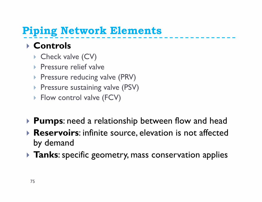
Piping Network Elements

� Controls� Check valve (CV)

� Pressure relief valve

� Pressure reducing valve (PRV)

� Pressure sustaining valve (PSV)

� Flow control valve (FCV)

� Pumps: need a relationship between flow and head

� Reservoirs: infinite source, elevation is not affected by demand

� Tanks: specific geometry, mass conservation applies

75

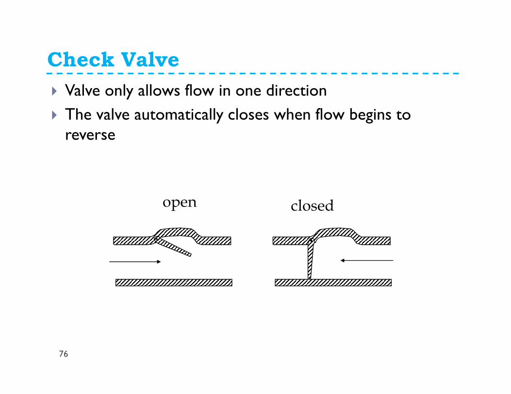
Check Valve

� Valve only allows flow in one direction

� The valve automatically closes when flow begins to reverse

closedopen

76

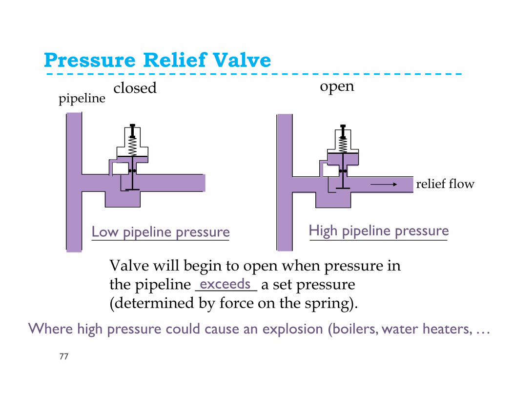
Pressure Relief Valve

Valve will begin to open when pressure in the pipeline ________ a set pressure (determined by force on the spring).

pipelineclosed

relief flow

open

exceeds

Low pipeline pressure High pipeline pressure

Where high pressure could cause an explosion (boilers, water heaters, …)

77

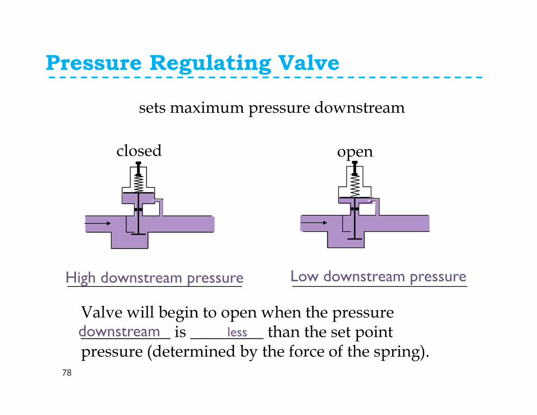
Pressure Regulating Valve

Valve will begin to open when the pressure ___________ is _________ than the set point pressure (determined by the force of the spring).

sets maximum pressure downstream

closed open

lessdownstream

High downstream pressure Low downstream pressure

78

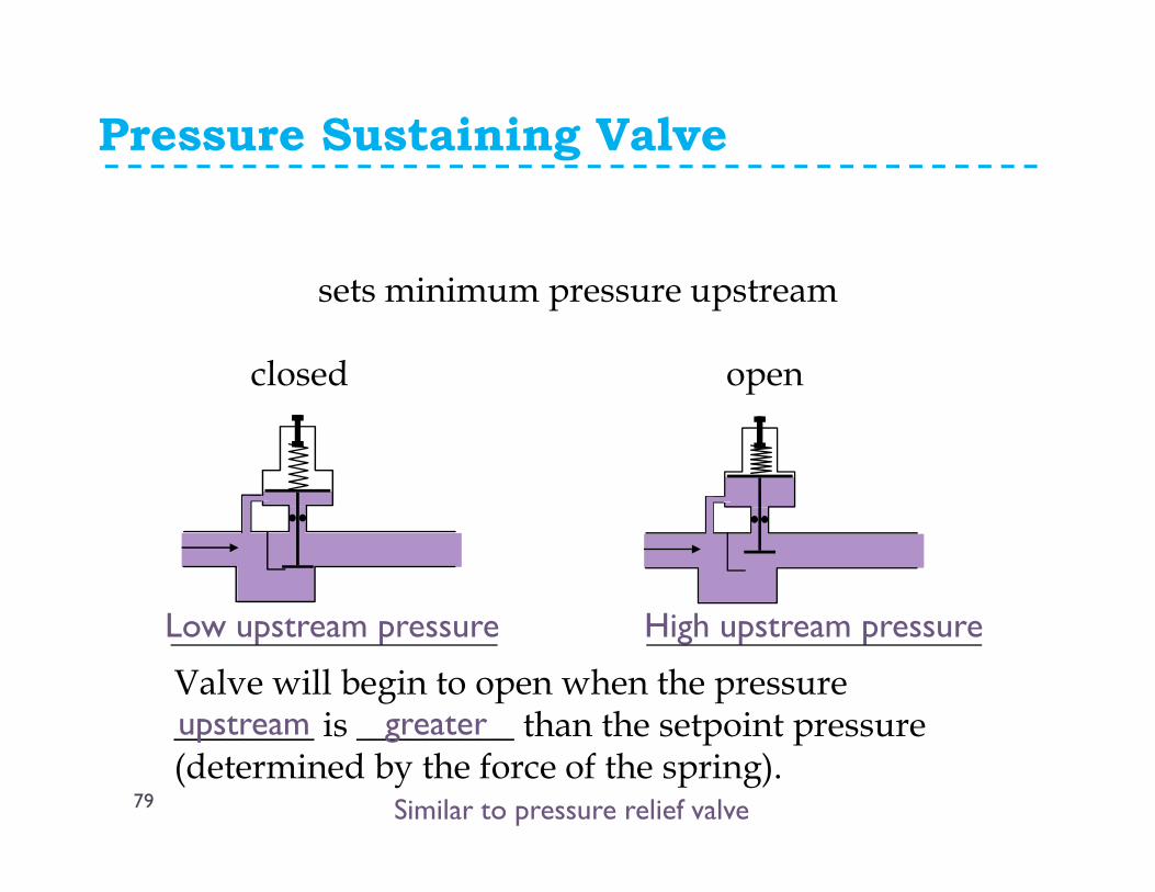
Pressure Sustaining Valve

Valve will begin to open when the pressure ________ is _________ than the setpoint pressure (determined by the force of the spring).

sets minimum pressure upstream

closed open

upstream greater

Low upstream pressure High upstream pressure

Similar to pressure relief valve79

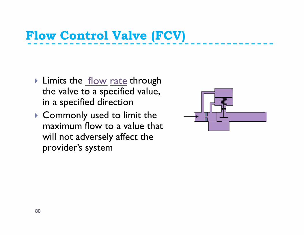
Flow Control Valve (FCV)

� Limits the ____ ___ through the valve to a specified value, in a specified direction

� Commonly used to limit the maximum flow to a value that will not adversely affect the provider’s system

flow rate

80

81

Thank You

Feel Free to Contact

Engineering

Water demand forecasting