Electronic copy available at: http://ssrn.com/abstract=1075862

Ecological Economics 27 (1998) 161–170

METHODS

A method for valuing global ecosystem services

Anne M. Alexander a,*, John A. List b, Michael Margolis a, Ralph C. d’Arge a

a Department of Economics and Finance, Uni6ersity of Wyoming, Laramie, WY 82071-3985, USAb Department of Economics, Uni6ersity of Central Florida, Orlando, FL 32816-1400, USA

Received 6 January 1997; received in revised form 22 September 1997; accepted 13 November 1997

Abstract

The goal of this paper is to provide an investigation of several approaches to valuing ecosystem services and tocontribute additional techniques which may be used in evaluating ‘green’ GDP accounts. Our estimates focus on theecosystem as a productive economic input, not a stock which is depreciated or depleted over time; as such, it differswith other concepts more frequently employed in green GDP accounting. Most of our results are derived from theanalytical fiction that a single owner of the biosphere establishes a market for all ecological resources. Thismonopolist then appropriates all rents from the human population. The maximum amount the monopolist chargesis first assumed to be world gross product less the global human subsistence level. In addition, we examine the excessrents available in factor markets using the assumption of weak complementarity between factor inputs and ecosystemservices. We also provide more conservative estimates of the value of ecosystem services by investigating thesustainable price the monopolist could charge the global population and by exploring the effects of compensatingwage differentials and a non-monopolist owner of the ecosystem. © 1998 Elsevier Science B.V. All rights reserved.

Keywords: Ecosystem services; Monopolist; Excess rents; Maximum surplus; Weak complementarity

1. Introduction

While it is ubiquitously acknowledged thatecosystems are essential to human existence,ecosystem services are typically unpriced or not

priced correctly at their marginal value because ofa lack of private, organized markets for suchservices. The absence of pricing mechanisms forthe ecosystem means that their contribution toour economy does not enter into most currentGross Domestic Product (GDP) accounts. Somecountries such as Sweden have tried to correct forthis by introducing ‘green’ GDP accounting. Typ-

* Corresponding author. Fax: +1 307 7665090; e-mail:aalex@uwyo.edu

0921-8009/98/$ - see front matter © 1998 Elsevier Science B.V. All rights reserved.

PII S0921-8009(97)00173-0

Electronic copy available at: http://ssrn.com/abstract=1075862

A.M. Alexander et al. / Ecological Economics 27 (1998) 161–170162

ically, their methods entail treating ecosystem ser-vices as a stock of inputs which are depreciated ordepleted over time. This methodology does notaccount for the productivity of ecological inputson which humans rely in economic pursuits. Thefact that the ecosystems’ value to our global econ-omy is not recognized or measured well has broadpolicy implications—the omission of its valueimplies the importance of the ecosystem may beignored in bottom-line policy decisions. Since theecosystem is a quintessential ingredient for eco-nomic activity, this exclusion is grossly negligent.Moreover, when the value of ecosystem servicesto land, labor, and capital productivity are disre-garded, these three factors are overvalued and theecosystem slighted in its contributions to ourglobal economy. Thus, when we speak of thevalue of ecosystem services in this study, we donot infer that a ‘price’ exists for ecosystem ser-vices (e.g. so the ecosystem can be bought andsold in the marketplace), rather, we intend tobring to light the very real economic value of theecosystem, which to date, is glaringly ignored incurrent national accounting practices.

In this paper, we use neoclassical economicmethods to examine several techniques of indi-rectly inferring a market value for ecosystem ser-vices to be included in green GDP accounts. Inkeeping with the spirit of GDP accounting, whichenumerates the value of payments made to factorsof production, the values we arrive at for ecosys-tem services are bounded above by gross worldproduct.1 The amount human society is pragmati-cally able to pay for ecosystem services cannotexceed world product because it is all that we canafford. Our investigation hinges on this assertion.We are not attempting to set a value for eachservice provided by the ecosystem, but rather areseeking the maximum amount that could feasiblybe paid for these services.2

Our attention is thus restricted to what Brown(1984) has called ‘economic values’.3 These valuesare assigned by a social process influenced bothby the context—chiefly markets, but also govern-ment and other collective procurement institu-tions—and by underlying ‘held values’, such asthe value associated with health enjoyed due toconsumption, or the beauty perceived in wildlands. Whether such economic value is an appro-priate measure of a resource’s contribution towelfare depends both on the legitimacy of the heldvalues and the accuracy with which they are cap-tured in this context. The legitimacy of held val-ues is a notion that economists almost universallyassume, or put aside as not amenable to logicalanalysis, but much of modern environmentalismhas consisted of attempts to influence held valuesso that stewardship and the health of other spe-cies are weighted more heavily. As for context, wehave no reason to believe that existing systems(i.e. representative government) for the purchaseof collective goods correctly capture citizens’ heldvalues. By restricting our attention to economicvalue we place all of these problems aside.

Our methods are also sensitive to assumptionsregarding the importance of ecosystem services inproduction and consumption processes. For ex-ample, if ecosystem services and other inputs,such as labor and capital, are readily substi-tutable, their value would be bounded above bythe cost of such substitution. If a dollar’s worth oflabor services could be substituted for ten units ofecological services, the value of ecological servicescould not exceed $0.10. Otherwise, labor serviceswould be partially or completely substituted forecological services.

The assumption we make is at the other ex-treme—ecological services are absolutely essentialin production and consumption. Their valuecould therefore be as great as the surplus gener-

every day, economic agents are implicitly valuing ecosystemservices daily (Costanza et al., 1997). Thus, research such asCostanza et al. (1997) and this endeavor represent first effortsto further our understanding of not only the value of allecosystem services, but also different approaches that can beimplemented to obtain this value.

3 We are grateful to an anonymous referee for bringingBrown’s taxonomy to our attention.

1 In particular, by the sum of all GDPs as currently calcu-lated �$18 trillion in 1987 (the year for which all calculationsare made). If all ecosystem services were priced through mar-kets, GDP would undoubtedly be quite different.

2 A hotly debated issue is whether we should place a valueon the ecosytem. Given individuals make ecosystem choices

Electronic copy available at: http://ssrn.com/abstract=1075862

A.M. Alexander et al. / Ecological Economics 27 (1998) 161–170 163

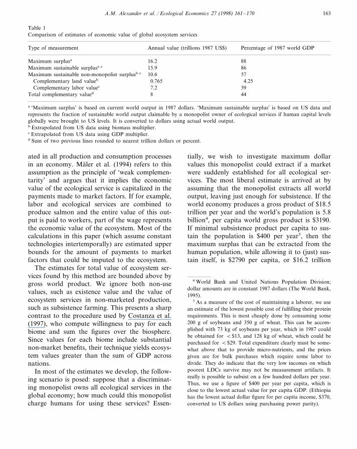
Table 1Comparison of estimates of economic value of global ecosystem services

Annual value (trillions 1987 US$) Percentage of 1987 world GDPType of measurement

Maximum surplusa 16.2 888615.9Maximum sustainable surplusa c

10.6 57Maximum sustainable non-monopolist surplusb c

0.765Complementary land valueb 4.25Complementary labor valuec 7.2 39

44Total complementary valued 8

a ‘Maximum surplus’ is based on current world output in 1987 dollars. ‘Maximum sustainable surplus’ is based on US data andrepresents the fraction of sustainable world output claimable by a monopolist owner of ecological services if human capital levelsglobally were brought to US levels. It is converted to dollars using actual world output.b Extrapolated from US data using biomass multiplier.c Extrapolated from US data using GDP multiplier.d Sum of two previous lines rounded to nearest trillion dollars or percent.

ated in all production and consumption processesin an economy. Maler et al. (1994) refers to thisassumption as the principle of ‘weak complemen-tarity’ and argues that it implies the economicvalue of the ecological service is capitalized in thepayments made to market factors. If for example,labor and ecological services are combined toproduce salmon and the entire value of this out-put is paid to workers, part of the wage representsthe economic value of the ecosystem. Most of thecalculations in this paper (which assume constanttechnologies intertemporally) are estimated upperbounds for the amount of payments to marketfactors that could be imputed to the ecosystem.

The estimates for total value of ecosystem ser-vices found by this method are bounded above bygross world product. We ignore both non-usevalues, such as existence value and the value ofecosystem services in non-marketed production,such as subsistence farming. This presents a sharpcontrast to the procedure used by Costanza et al.(1997), who compute willingness to pay for eachbiome and sum the figures over the biosphere.Since values for each biome include substantialnon-market benefits, their technique yields ecosys-tem values greater than the sum of GDP acrossnations.

In most of the estimates we develop, the follow-ing scenario is posed: suppose that a discriminat-ing monopolist owns all ecological services in theglobal economy; how much could this monopolistcharge humans for using these services? Essen-

tially, we wish to investigate maximum dollarvalues this monopolist could extract if a marketwere suddenly established for all ecological ser-vices. The most liberal estimate is arrived at byassuming that the monopolist extracts all worldoutput, leaving just enough for subsistence. If theworld economy produces a gross product of $18.5trillion per year and the world’s population is 5.8billion4, per capita world gross product is $3190.If minimal subsistence product per capita to sus-tain the population is $400 per year5, then themaximum surplus that can be extracted from thehuman population, while allowing it to (just) sus-tain itself, is $2790 per capita, or $16.2 trillion

4 World Bank and United Nations Population Division;dollar amounts are in constant 1987 dollars (The World Bank,1995).

5 As a measure of the cost of maintaining a laborer, we usean estimate of the lowest possible cost of fulfilling their proteinrequirements. This is most cheaply done by consuming some200 g of soybeans and 350 g of wheat. This can be accom-plished with 73 kg of soybeans per year, which in 1987 couldbe obtained for B$13, and 128 kg of wheat, which could bepurchased for B$29. Total expenditure clearly must be some-what above that to provide micro-nutrients, and the pricesgiven are for bulk purchases which require some labor todivide. They do indicate that the very low incomes on whichpoorest LDCs survive may not be measurement artifacts. Itreally is possible to subsist on a few hundred dollars per year.Thus, we use a figure of $400 per year per capita, which isclose to the lowest actual value for per capita GDP. (Ethiopiahas the lowest actual dollar figure for per capita income, $370,converted to US dollars using purchasing power parity).

A.M. Alexander et al. / Ecological Economics 27 (1998) 161–170164

globally. We call this amount the ‘Maximum Sur-plus’ the monopolist could charge (Table 1).

The remainder of this paper is organized asfollows. In Section 2, we estimate the value ofecosystem services captured in compensation toworkers. Section 3 presents the parallel calcula-tion for land rents. Section 4 consists of tworefinements on the ‘Maximum Surplus’ calculatedabove, allowing for the need to replace humanand physical capital and the possibility of incom-plete market power. For purposes of comparison,Section 5 presents an alternative estimate of thevalue of ecosystem services captured in wages. Allestimates are made using US data, on the (per-haps chauvinistic) grounds that institutional ine-fficiencies are minimal in the United States. Theestimates are then scaled, using either GDP orbiomass multipliers, to a global valuation.

2. Capitalization of wages

Imagine that the biosphere is owned by a mo-nopolist who can extract all rents6, which mightotherwise accrue through the labor market to thehuman population. Assume that labor and eco-logical services are weak complements in produc-tion; the necessity of ecosystem services in theproductivity of labor is then reflected by the sur-pluses currently accruing to the labor force. Theestimated ecosystem value using this approachrepresents an upper bound for the total value ofecosystem services now captured by workers. Theestimate is given by Eq. (1):

Ecosystem value+Subsistence wage

=Total wage bill, (1)

where the subsistence wage is taken to be $400 percapita per year, as given in the introduction. In1994, there were 87379000 full-time workers with

median weekly wages of $4677, and 26050000part-time workers with median weekly wages of$385 (US Department of Commerce, Census ofthe Population, 1995). Assuming each full-timelaborer works for 52 weeks per year, annual in-come for full-time workers is $24284, or $18855in 1987 dollars. Subtracting the yearly subsistencevalue of $400 per worker implies that $1.6 trillioncan be extracted from the full-time work force.Also, if part-time workers cannot be made towork full time (many are performing householdservices essential to subsistence), $6622 can beextracted from each part-time worker, for a totalof $0.2 trillion. Therefore, the surplus the monop-olist could extract from the entire US workerpopulation is $1.8 trillion. This figure is scaled tothe global level by multiplying it by four, on thegrounds that 1987 GDP in the US was 25% ofglobal gross product. Ecosystem services, as capi-talized in the wage bill, are thus estimated at $7.2trillion annually. This is reported in Table 1 as‘Complementary Labor Value’.

3. Land rent differentials

In this section we present an estimate of thevalue of ecosystem services captured in the privateland market. We focus on agricultural land, asrents associated with other uses of land are possi-bly included in the estimate of compensating wagedifferentials in Section 5. The definition of agri-cultural land utilized in this section follows thatused to designate ‘Land in Farms’ by the USDepartment of Commerce, Bureau of Census(1982, 1992), in their Census of Agriculture.

Agricultural production requires that land becombined with other inputs we divide into twocategories: man-made inputs and ecological ser-vices. Ecological services include soil salinity andpermeability, annual rainfall, soil microbes andaverage temperatures—any attribute naturally oc-curring in and around land. Man-made inputs

6 The term ‘rent’, as used by economists, refers to theamount paid for a service over the minimum that would haveto be paid to attract the resources needed to produce thatservice. In most examples in this paper, the human populationhas no alternative employment outside of dealing with theowner of the biosphere, so anything paid to humans abovewhat it takes to keep the workforce reproducing is ‘rent’.

7 Dollar amounts were converted to 1987 dollars for com-parability using the GDP deflator reported in the Budget ofthe United States, Fiscal Year 1997, Historical Tables (USGeneral Accounting Office, 1997).

A.M. Alexander et al. / Ecological Economics 27 (1998) 161–170 165

include fertilizer, machinery and labor, all ofwhich are priced in markets. The land itself is alsopriced in markets, but ecological services are not.Since ecological services are critical in determiningdemand and best use for agricultural land, there islikely to be weak complementarity between landand ecosystem services. Given usable data on landprices, we could make a calculation parallel tothat made above for labor by subtracting fromland prices the amount representing man-madeinputs that are sold with land. We do not havesuch data and therefore use the following alterna-tive scheme.

Agricultural output markets are close to per-fectly competitive, so farmers should earn zerorents from production. This implies that the dif-ference between annual gross value (price timesoutput) and total factor payments should be zero.Man-made factor inputs are easily valued sincethey are priced in private markets. Thus, from thezero-rent assumption, any positive residual valueremaining after subtracting market-priced factorpayments from the annual gross value of a farm isthe total use value of ecological services in agri-cultural production. Hence:

Ecosystem value+Production expenses

=Value of output, (2)

Production expenses reflect the market value ofman-made inputs. We use average per acre ex-penses of $135 per acre8 and the value of outputfor the two top crops in the US to calculate theresidual value of ecosystem services in Eq. (2).

Total corn crops are the highest crop-use per-centage of all crops in the US and occupy 15% ofall arable land in the US.9 Corn also had thehighest value of production of all crops in theUnited States in 1995. The state with the highestvalue of yield per acre for corn crops is Iowa,where corn land yields $291 per acre.10 Subtract-ing production costs of $135/acre, the net surplusof corn production in Iowa is :$156/acre. Thestate with the lowest value yield per acre in corn isMontana, where net surplus is $145/acre.11 Thus,for the 70.29 million acres of corn land in the US,the total value of ecological services is :$10–11billion.

The other crop we consider is soybeans, whichoccupies �13% of all arable US land. The statewith the highest value of soybean yield per acre in1995 is again Iowa, where surplus was $65 peracre in 1995.12 The state with the lowest value ofsoybean production was Florida, which yieldedexcess rents close to zero. Approximately 60.6million acres are devoted to production of soy-beans in the US, giving an upper bound valuationof ecological services in the production of soy-beans equal to $4 billion. Adding this to ourestimate for corn, at least 28% of the arable landin the US benefits from ecological services with atotal value of $14–15 billion per year.

To scale this number into a global ecologicalservice value for agricultural land, we first multi-ply by 1/0.28 to estimate an upper bound on thevalue of ecosystem services enjoyed by all farmersin the US. The resulting figure is multiplied by1/0.07 to derive the value that could be enjoyed ifUS farming was extended to the rest of the world.The biomass multiplier, 1/0.07, is obtained via thefact that the US contains �7% of the world’s

8 Expenses included in our calculations include: seeds, bulbsand trees added; commercial fertilizer; other commercial chem-icals; machinery hire; feed purchases; hired labor; contractlabor; energy and other petroleum products; and interestexpenses for farm business. The total value of these expenses isreported in the Census, as is the number of farms incurringeach of the expenses. Using these numbers, we compute aver-age expenses per farm as $61097 in 1982. Accounting forinflation using the Producer Price Index for farm products,inflation-adjusted average per farm expenses for 1987 are$63358. Additionally, according to the US Department ofAgriculture, the average acreage for a US farm is 469 acres.This information yields the average per acre expenses numberused in our calculations.

9 CIA World Factbook 1995, (US Central IntelligenceAgency, 1995) and US Department of Agriculture, Agricul-tural Statistics 1995–96 (US Department of Agriculture,1995–1996).

10 123 bushels per acre×$3.05/bushel (USDA) times theGDP deflator of 0.776.

11 120 bushels/acre, $3.00 per bushel in 1995 prices.12 43 bushels per acre, $6.75/bushel in 1995 prices.

A.M. Alexander et al. / Ecological Economics 27 (1998) 161–170166

continental biomass (Continental biomass is theappropriate measure since the only type of agri-culture we consider here is completely land-based). This figure is in turn based on roughmeasurements of the amount of area covered byeach of seven biomes13 and the average biomassdensities for each biome (Begon et al., 1986).Multiplication by these numbers gives a totalvalue of $765 billion.

The last row of Table 1 reports the summationof values captured in wages and land rents andlabels this value as ‘Total Complementary Value’.There is fear that some ecosystem services havethus been counted twice, but we believe that perilto be minimal. Double counting occurs to theextent that profit of farm owners is counted inwage calculations, but not subtracted as a cost tothe farm. This would likely have been a seriousproblem a century ago, but family farmers arenow B3% of the labor force.14 Further evidencethat this potential upward bias is minute is pro-vided by our alternative calculations below, whichall yield values well above the total complemen-tary value.

4. Steady state capital flows

The maximum surplus suggested in the intro-duction and calculated by subtracting subsistenceincome from world product is a surplus thatcannot be sustained. Just as it is necessary to feedworkers to obtain a full year of output, it isnecessary to rebuild capital and train new genera-tions of workers if the stream of output is to beproduced in perpetuity. The calculations beloware intended to indicate how great a differencethis sustainability constraint will make to the totalvaluation of ecological services.

In the case of a monopolist owner of ecologicalservices, the only subtraction that must be madefor physical capital is the cost of building newmachines to replace those which wear out orbecome obsolete. We know of no data series thatcorresponds to this cost precisely. What we wouldlike is a solution to the problem of maximizingoutput subject to a sustainability constraint; thatis, the requirement that real production is con-stant in perpetuity. The numbers reported undercapital depreciation in GDP (which are intendedto capture the amount of capital value lost inroutine wear and tear) are more similar to thesolution to the problem of minimizing tax bur-dens subject to a legal constraint. Congress andthe Internal Revenue Service determine the frac-tion of total capital value firms may deduct frompre-tax income for several categories of equip-ment; firms then choose equipment types withthese tax advantages in mind. Actual deteriora-tion of physical capital is approximated only tothe extent that the coefficients in the tax-coderepresent actual rates of wear and tear. Even thisimperfect measure is calculated completely onlyfor the manufacturing industry.

Nevertheless, the total annual rate of capitaldepreciation reported in the 1987 Census of Man-ufacturers was $63 billion (US Department ofCommerce, Bureau of Census, 1987). To this weadd the cost of capital rented in the accountant’ssense, another $15.6 billion15 to conclude thatsome $76.6 is required to maintain the industrialbase.16 To calculate from this manufacturingfigure, a number for the whole economy, we haveonly the roughest of techniques. Manufacturing

15 Any piece of capital owned by one manufacturer andrented to another would therefore be double-counted. It seemsprobable, however, that most rented machinery is owned byfirms in the rental business, which falls into the category ofservices.

16 This is within $100 million of (manufacturers) reportedspending on new capital in the same census. This latter figureshould include spending dedicated to the expansion, as well asmaintenance, of the manufacturing base. But, since the totalvalue of the manufacturing capital stock rose by only $15billion during all of the 1980s (US Department of Commerce,Bureau of Census, 1995 Table 1245), any correction is mostlikely small.

13 We assume the US contains �25% of the world’s temper-ate grassland, 25% of its temperate deciduous forest, 20% ofits temperate evergreen forests, 11% of its desert/semidesertregions, 10% of its swamp and marshlands, 9% of its culti-vated land, and 5% of its chaparral biome. These assumptionsrender an estimate that the US contains :127.1 metric tonsof biomass.

14 US Department of Commerce, Census of the Population(1995).

A.M. Alexander et al. / Ecological Economics 27 (1998) 161–170 167

contributes less than one-third of total US GDP;it is, however, much more capital intensive thanservice sectors. In keeping with the goal of findinga maximum surplus, we seek the minimum rea-sonable deduction for depreciation. Doubling themanufacturing number seems an appropriatelyconservative deduction. Thus, having subtractedfrom GDP the minimum wage bill and that partof land rents not paying for ecosystem services,we subtract another $160 billion to find the maxi-mum surplus.

By way of a consistency check on this number,the total value of industrial machinery and equip-ment sold in the census year was roughly $218billion, while the total value of transport equip-ment was $333 billion. If all purchased machinerywere used domestically to replace worn out equip-ment, it would imply a deduction four times asgreat as that calculated from our depreciationfigure. Only about $0.12 billion worth of this wasexported (US Department of Commerce, Bureauof Census, 1995, Statistical Abstract for the US,Table 1255) and the transportation sector appearsto be increasing its capital stock at a rate of $15billion per year (US Department of Commerce,Bureau of Census, 1995, Table 875). Since manu-facturing expanded very little (US Department ofCommerce, Bureau of Census, 1995, StatisticalAbstract for the US, Table 1255), the alternativefigure should be well above our $160 billion esti-mate. This increases our confidence that the figureis a lower bound on the deduction required forsustainability of the capital stock.

We now turn to sustaining the human capitalstock of the economy. The cost of sustenanceshould include some valuation of the total cost ofparental time, some fraction of health care expen-ditures, production sacrificed to reduce childhoodexposure to lead and several tens of thousands ofsimilar items. These are undoubtedly valuable in-puts but they are not priced in markets. Thus, weview the stock of human capital as if it weresimply a stock of educational attainment. Assuch, the stock currently consists of 55.7 millionhigh school graduates, 20.8 million holders ofbachelors degrees, 7.5 million masters degrees,2.75 million professional degrees, and 1.2 milliondoctorates (US Department of Commerce, Bu-

reau of Census, 1995 Table 545). The cost of ayear of education for a child is �$360017, al-though this would surely be much lower if teach-ers and administrators were earning subsistencewages (a similar qualification applies to the costof producing physical capital). We will use thisdollar figure for all levels of education.

For our calculations, we assume that a highschool graduate must be replaced every 50 years,a college graduate every 44 years, a master orprofessional every 41 years and a doctorate every40 years. These assumptions are made by sub-tracting an estimated age of attainment of thesedegrees18 from the normative retirement age of 68.Therefore, maintaining the human capital stockrequires the creation of 1.15 million high schoolgraduates, 0.47 million college graduates, a quar-ter million masters and professionals and 30000doctorates each year. The assumption of constantcost per year of education and the same assump-tion on the time taken to attain each degreeindicates each high school graduate will cost �$47000; each college graduate �$68000; eachmaster or professional $79000; and each doctor-ate $82000. This yields a human capital replace-ment bill of $105.8 billion per year. Extrapolatingthese numbers to the rest of the world and sub-tracting from ‘Maximum Surplus’, the total re-quired to sustain human and physical capital givesthe $15.9 trillion reported as ‘Maximum Sustain-able Surplus’, in Table 1. Our conservative esti-mates of what is required to sustain capital resultin only an insignificant reduction in the amount amonopolist could extract from the human popula-tion. The more liberal estimate of physical capitalneeds implied by the total value of equipmentsales would reduce this amount by less than one-fourth of one percent.

17 US Bureau of the Census 1995, Table 245. Converted to1987 dollars with the GDP deflator from Budget of the UnitedStates, Fiscal Year 1997, Historical Tables (US General Ac-counting Office, 1997).

18 We assume high school can be completed at age 18 andthat other degrees can be earned in the average times reportedin US Department of Commerce, Bureau of Census (1995),Statistical Abstract of the United States, Tables 295–297.

A.M. Alexander et al. / Ecological Economics 27 (1998) 161–170168

A further calculation assumes that the servicesof nature are not purely complementary to otherfactors of production. If this is the case, thehypothetical owner of ecological services is un-likely to enjoy the complete market power as-sumed in our previous calculations. To give arough indication of how much might nonethelessbe charged for ecological services, we subtractfrom the above payments which would have to bemade to owners of labor and capital in a marketeconomy. Clearly, these are less than the actualpayments made to U.S. workers and owners ofcapital, which include some of the returns to theunowned environment. As to how much less, weuse the following set or rather ad hoc assumptionsfor demonstrative purposes. Suppose that a typi-cal worker earns the same wage as an Italianworker19 and that a capital owner earns 12% onher resource. Assuming these factors are thenused as productively as in the US, owners ofnature would collectively earn the amount re-ported in Table 1 as ‘Maximum Sustainable Non-Monopolist Surplus’.

5. Compensating wage differentials

This section uses results from Blomquist et al.(1988) to estimate a value for ecosystem servicesthat is capitalized in the wage and housing mar-kets. Unlike the results in Table 1, values calcu-lated in this section are for services provided byecosystems directly to consumers; that is, we arenow valuing inputs to consumption rather thanproduction. One might think, therefore, that theseestimates should be added to the numbers derivedso far to find a total value for ecosystem services,but that would be erroneous—values to house-holds are conditional on household income, whichincludes excess rents due to ecosystem services.Our purpose in presenting these numbers ismerely to indicate the likely relative importance ofthese non-market ecosystem benefits.

The techniques used here are due to Rosen(1979), who suggested that locations are best

viewed as tied bundles of wages, rents and ameni-ties. More recently, evidence of the influence ofamenities on wages has been researched byRoback (1982), Graves (1983) and Blomquist etal. (1988), amongst others. Their findings suggestthat wages are negatively affected by positiveamenities and positively affected by negativeamenities (workers are generally willing to give uphigher wages to live in more amenity-richregions).20

Amenities and disamenities in the Blomquist etal. (1988) study, that we assume are ecologicalservices, include average precipitation per year,humidity, heating degree days per year, coolingdegree days per year, average wind speed (milesper hour), sunshine (days per year), and proximityto coast. Blomquist et al. (1988) found that pre-cipitation, sunshine and access to the coast aremarginal net amenities—that is, the wage differ-ential in the presence of these ecological factors isnegative, implying workers are willing to acceptlower wages to live in regions with greater accessto these amenities. Humidity, heating degree days,cooling degree days and wind speed are found tobe marginal net disamenities. Workers in regionswith greater amounts of these disamenities willreceive higher wages, ceteris paribus.

An upper bound can be obtained by assumingone US county represents ‘Nirvana’, which ischaracterized by the ‘best’ bundle of ecologicalamenities/disamenities found in Blomquist et al.(1988). Nirvana would then be characterized byhaving access to the coast, healthy annual precipi-tation, higher-than-average days of sunshine, lowwind speed, lower-than-average heating and cool-ing degree days and low humidity. Similarly, weconstruct a fictional county with the worst possi-ble amenity/disamenity bundle (‘Low County’)and one with the mean level of every amenity and

20 An anonymous referee pointed out that the value of agiven amenity will vary across people; and it may even be thecase that one person’s amenity is another’s disamenity. Thispoint is correct, but we may nonetheless speak unambiguouslyof the value of an amenity as its value to the person whovalues it most—that is, the agent who would own the amenityif the amenity were marketed. This same problem applies toconventional private goods and the same solution was foundby the classical economists (Jevons, 1879; Walras, 1831).

19 About $15800 per year, according to Reddy (1994), p.457.

A.M. Alexander et al. / Ecological Economics 27 (1998) 161–170 169

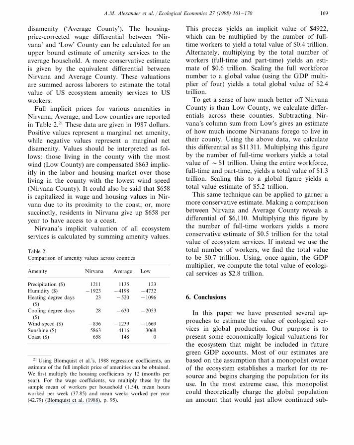
disamenity (‘Average County’). The housing-price-corrected wage differential between ‘Nir-vana’ and ‘Low’ County can be calculated for anupper bound estimate of amenity services to theaverage household. A more conservative estimateis given by the equivalent differential betweenNirvana and Average County. These valuationsare summed across laborers to estimate the totalvalue of US ecosystem amenity services to USworkers.

Full implicit prices for various amenities inNirvana, Average, and Low counties are reportedin Table 2.21 These data are given in 1987 dollars.Positive values represent a marginal net amenity,while negative values represent a marginal netdisamenity. Values should be interpreted as fol-lows: those living in the county with the mostwind (Low County) are compensated $863 implic-itly in the labor and housing market over thoseliving in the county with the lowest wind speed(Nirvana County). It could also be said that $658is capitalized in wage and housing values in Nir-vana due to its proximity to the coast; or, moresuccinctly, residents in Nirvana give up $658 peryear to have access to a coast.

Nirvana’s implicit valuation of all ecosystemservices is calculated by summing amenity values.

This process yields an implicit value of $4922,which can be multiplied by the number of full-time workers to yield a total value of $0.4 trillion.Alternately, multiplying by the total number ofworkers (full-time and part-time) yields an esti-mate of $0.6 trillion. Scaling the full workforcenumber to a global value (using the GDP multi-plier of four) yields a total global value of $2.4trillion.

To get a sense of how much better off NirvanaCounty is than Low County, we calculate differ-entials across these counties. Subtracting Nir-vana’s column sum from Low’s gives an estimateof how much income Nirvanans forego to live intheir county. Using the above data, we calculatethis differential as $11311. Multiplying this figureby the number of full-time workers yields a totalvalue of �$1 trillion. Using the entire workforce,full-time and part-time, yields a total value of $1.3trillion. Scaling this to a global figure yields atotal value estimate of $5.2 trillion.

This same technique can be applied to garner amore conservative estimate. Making a comparisonbetween Nirvana and Average County reveals adifferential of $6,110. Multiplying this figure bythe number of full-time workers yields a moreconservative estimate of $0.5 trillion for the totalvalue of ecosystem services. If instead we use thetotal number of workers, we find the total valueto be $0.7 trillion. Using, once again, the GDPmultiplier, we compute the total value of ecologi-cal services as $2.8 trillion.

6. Conclusions

In this paper we have presented several ap-proaches to estimate the value of ecological ser-vices in global production. Our purpose is topresent some economically logical valuations forthe ecosystem that might be included in futuregreen GDP accounts. Most of our estimates arebased on the assumption that a monopolist ownerof the ecosystem establishes a market for its re-source and begins charging the population for itsuse. In the most extreme case, this monopolistcould theoretically charge the global populationan amount that would just allow continued sub-

Table 2Comparison of amenity values across counties

LowAmenity AverageNirvana

11351211Precipitation ($) 123−1923 −4732Humidity ($) −4198

−109623Heating degree days −520($)

Cooling degree days −205328 −630($)

−1669−836 −1239Wind speed ($)30684116Sunshine ($) 5863

Coast ($) 658 148 0

21 Using Blomquist et al.’s, 1988 regression coefficients, anestimate of the full implicit price of amenities can be obtained.We first multiply the housing coefficients by 12 (months peryear). For the wage coefficients, we multiply these by thesample mean of workers per household (1.54), mean hoursworked per week (37.85) and mean weeks worked per year(42.79) (Blomquist et al. (1988), p. 95).

A.M. Alexander et al. / Ecological Economics 27 (1998) 161–170170

sistence. If the ecosystem is purely complementaryto other factors of production, the monopolistcould extract all excess rents currently accruing toowners of the other factors.

We also incorporate a sustainability constraintinto our estimates, allowing capital stocks to bereplenished over time. The resulting figures aremuch lower than those calculated above, but ap-pear to be more reasonable given capital stocksprobably have to be replenished over time tomaintain sustainable production. In addition toinvestigating these ‘maximum surplus’ and ‘com-plementary value’ estimates, we also explore thevalue of ecosystem services using compensatingwage differential data and a non-monopolist rentsassumption in order to obtain more conservativeestimates. All of these estimates are bounded logi-cally by zero on the lower end and gross worldoutput at the upper end. Our estimates suggestthat ecological services are worth between 44 and88% of total world output.

Although our findings are much lower thanestimates found by Costanza et al. (1997), theunderlying message is clearly similar—includingthe value of the ecosystem would dramaticallyalter current GDP estimates. Our approach differsfrom concepts more frequently endorsed in greenGDP accounting, such as inclusion of ‘deprecia-tion’ or depletion of natural resource stocks, inthat it calls direct attention to the productivecontribution of ecosystem services as a whole.Nevertheless, results from our numerous estima-tion techniques emphasize the importance of in-clusion of the ecosystem in current GDPaccounts.

Acknowledgements

We wish to thank Robert Costanza, partici-pants at the University of California-Santa Bar-bara National Center for Ecological Analysisworkshop, ‘The Total Value of the World’sEcosystem Services and Natural Capital’, andthree anonymous referees for their helpful com-

ments on previous drafts. All remaining errors arethe sole responsibility of the authors.

References

Begon, M., Harper, J.L, Townsend, C.R., 1986. Ecology:Individuals, Populations, & Communities, 1. Blackwell,Boston.

Blomquist, G., Berger, M., Hoehn, J., 1988. New Estimates ofthe Quality of Life in Urban Areas. Am. Econ. Rev. 78,89–107.

Brown, T., 1984. The Concept of Value in Resource Alloca-tion. Land Econ. 60, 1–23.

Costanza, R., d’Arge, R., de Groot, R., Farber, S., Grasso,M., Hannon, B., Limburg, K., Naeem, S., O’Neill, R.,Paruelo, J., Raskin, R., Sutton, P., van den Belt, M., 1997.The value of the world’s ecosystem services and naturalcapital. Nature 387, 253–260.

Graves, P.E., 1983. Migration with a composite commodity:The role of rents. J. Reg. Sci. 23, 541–546.

Jevons, W.S., 1879. The Theory of Political Economy.Macmillan, London.

Maler, K.G., Gren, I., Folke, C., 1994. Multiple use of envi-ronmental resources: A household production functionapproach to valuing natural capital. In: Jansson, A., et al.(Eds.), Investing in Natural Capital: The Ecological Eco-nomics Approach to Sustainability. Island Press, Washing-ton, DC, pp. 233–249.

Reddy, Marlita A. (Ed.), 1994. Statistical Abstract of theWorld. Gale Research. Detroit.

Roback, J., 1982. Wages, rents the quality of life. J. Polit.Econ. 90, 1257–1278.

Rosen, S., 1979. Wage-based indexes of urban quality of life.In: Miezkowski, P., Straszheim, M. (Eds.), Current Issuesin Urban Economics. John Hopkins Press, Baltimore, MD,pp. 74–104.

US Central Intelligence Agency, 1995. C.I.A. World Fact-book.

US Department of Agriculture, 1995–1996. AgriculturalStatistics.

US Department of Commerce, Bureau of Census, 1982, 1992.Census of Agriculture.

US Department of Commerce, Bureau of Census, 1987. Cen-sus of Manufacturers.

US Department of Commerce, Bureau of Census, 1995. Cen-sus of the Population.

US Department of Commerce, Bureau of Census, 1995. Statis-tical Abstract of the United States.

US General Accounting Office, 1997. Budget of the UnitedStates, Fiscal Year 1997, Historical Tables.

Walras, A.A., 1831. De la nature de la richesse et de l’originede la valeur. Johanneau, Paris.

The World Bank, 1995. World Bank Atlas.

.