Download pdf - A PARTICLE SWARM OPTIMIZATION FOR THE VEHICLE ROUTING PROBLEM

University of Rhode IslandDigitalCommons@URI

Open Access Dissertations

2014

A PARTICLE SWARM OPTIMIZATION FORTHE VEHICLE ROUTING PROBLEMChoosak PornsingUniversity of Rhode Island, [email protected]

Follow this and additional works at: http://digitalcommons.uri.edu/oa_diss

Part of the Industrial Engineering Commons

Terms of UseAll rights reserved under copyright.

This Dissertation is brought to you for free and open access by DigitalCommons@URI. It has been accepted for inclusion in Open Access Dissertationsby an authorized administrator of DigitalCommons@URI. For more information, please contact [email protected].

Recommended CitationPornsing, Choosak, "A PARTICLE SWARM OPTIMIZATION FOR THE VEHICLE ROUTING PROBLEM" (2014). Open AccessDissertations. Paper 246.

http://digitalcommons.uri.edu?utm_source=digitalcommons.uri.edu%2Foa_diss%2F246&utm_medium=PDF&utm_campaign=PDFCoverPages

http://digitalcommons.uri.edu/oa_diss?utm_source=digitalcommons.uri.edu%2Foa_diss%2F246&utm_medium=PDF&utm_campaign=PDFCoverPages

http://digitalcommons.uri.edu/oa_diss?utm_source=digitalcommons.uri.edu%2Foa_diss%2F246&utm_medium=PDF&utm_campaign=PDFCoverPages

http://network.bepress.com/hgg/discipline/307?utm_source=digitalcommons.uri.edu%2Foa_diss%2F246&utm_medium=PDF&utm_campaign=PDFCoverPages

http://digitalcommons.uri.edu/oa_diss/246?utm_source=digitalcommons.uri.edu%2Foa_diss%2F246&utm_medium=PDF&utm_campaign=PDFCoverPages

mailto:[email protected]

A PARTICLE SWARM OPTIMIZATION FOR THE VEHICLE ROUTING

PROBLEM

BY

CHOOSAK PORNSING

A DISSERTATION SUBMITTED IN PARTIAL FULFILLMENT OF THE

REQUIREMENTS FOR THE DEGREE OF

DOCTOR OF PHILOSOPHY

IN

INDUSTRIAL ENGINEERING

UNIVERSITY OF RHODE ISLAND

2014

DOCTOR OF PHILOSOPHY DISSERTATION

OF

CHOOSAK PORNSING

APPROVED:

Dissertation Committee:

Major Professor Manbir S. Sodhi

Frederick J. Vetter

Gregory B. Jones

Nasser H. Zawia

DEAN OF THE GRADUATE SCHOOL

UNIVERSITY OF RHODE ISLAND

2014

ABSTRACT

This dissertation is a study on the use of swarm methods for optimization,

and is divided into three main parts. In the first part, two novel swarm meta-

heuristic algorithms—named Survival Sub-swarms Adaptive Particle Swarm Op-

timization (SSS-APSO) and Survival Sub-swarms Adaptive Particle Swarm Opti-

mization with velocity-line bouncing (SSS-APSO-vb)—are developed. These new

algorithms present self-adaptive inertia weight and time-varying adaptive swarm

topology techniques. The objective of these new approaches is to avoid premature

convergence by executing the exploration and exploitation stages simultaneously.

Although proposed PSOs are fundamentally based on commonly modeled behav-

iors of swarming creatures, the novelty is that the whole swarm may divide into

many sub-swarms in order to find a good source of food or to flee from predators.

This behavior allows the particles to disperse through the search space (diversi-

fication) and the sub-swarm with the worst performance dies out while that the

best performance grows by producing offspring. The tendency of an individual

particle to avoid collision with other particles by means of simple neighborhood

rules is retained in this algorithm. Numerical experiments show that the new

approaches outperform other competitive algorithms by providing the best solu-

tions on a suite of standard test problem with a much higher consistency than the

algorithms compared.

In the second part, the SSS-APSO-vb is used to solve the capacitated vehicle

routing problem (CVRP). To do so, two new solution representations—the con-

tinuous and the discrete versions—are presented. The computational experiments

are conducted based on the well-known benchmark data sets and compared to two

notable PSO-based algorithms from literature. The results show that the proposed

methods outperform the competitive PSO-based algorithms. The continuous PSO

works well with the small-size benchmark problems (the number of customers is

less than 75), while the discrete PSO yields the best solutions with the large-size

benchmark problem (the number of customers is more than 75). The effectiveness

of the proposed methods is enhanced by the strength mechanism of the SSS-APSO-

vb, the search ability of the controllable noisy-fitness evaluation, and the powerful

but cheapest cost of the common local improvement methods.

In the third part, a particular reverse logistics problem—the partitioned ve-

hicle of a multi commodity recyclables collection problem—is solved by a variant

of PSO, named Hybrid PSO-LR. The problem is formulated as the generalized

assignment problem (GAP) in which is solved in three phases: (i) construction of

a cost allocation matrix, (ii) solving an assignment problem, and (iii) sequencing

customers within routes. The performance of the proposed method is tested on

randomly generated problems and compared to PSO approaches (sequential and

parallel) and a sweep method. Numerical experiments show that Hybrid PSO-LR

is effective and efficient for the partitioned vehicle routing of a multi commodity

recyclables collection problem. This part also shows that the PSO enhances the

LR by providing exceptional lower bounds.

ACKNOWLEDGMENTS

First of all I would like to express my gratitude to Professor Dr. Manbir

Sodhi, my major advisor, who gave me the opportunity to do my PhD in his

research group and introduced me an amazing optimization tool, Particle Swarm

Optimization. Thank you for his outstanding support and for proving ideas and

guidance whenever I was facing difficulties during my journey. I am also very

grateful to the committee members—Dr. Gregory B. Jones, Dr. Frederick J.

Vetter, Dr. David G. Taggart, Dr. Todd Guifoos, and Dr. Thomas S. Spengler

for their support and encouragement as well as the valuable inputs towards my

research.

I also owe gratitude to all my colleagues from the research group at Depart-

ment of Mechanical, Industrial & Systems Engineering, the University of Rhode

Island. Thank you for exchanging scientific ideas and providing helpful suggestions.

It is a pleasure working with you.

Special thanks to all members of my family: dad, mom, and brother for all

their support; especially, my wife and my son, Uriawan and Chindanai. They are

my inspiration.

iv

To my parents, Suthep Pornsing and Kimyoo Pornsing; and my family, Urai-

wan Pornsing and Chindanai Pornsing.

v

TABLE OF CONTENTS

ABSTRACT . . . . . . . . . . . . . . . . . . . . . . . . . . . . . . . . . . ii

ACKNOWLEDGMENTS . . . . . . . . . . . . . . . . . . . . . . . . . . iv

DEDICATION . . . . . . . . . . . . . . . . . . . . . . . . . . . . . . . . . v

TABLE OF CONTENTS . . . . . . . . . . . . . . . . . . . . . . . . . . vi

LIST OF TABLES . . . . . . . . . . . . . . . . . . . . . . . . . . . . . . . x

LIST OF FIGURES . . . . . . . . . . . . . . . . . . . . . . . . . . . . . . xii

CHAPTER

1 Introduction . . . . . . . . . . . . . . . . . . . . . . . . . . . . . . . 1

1.1 Motivation . . . . . . . . . . . . . . . . . . . . . . . . . . . . . . 2

1.2 Objectives . . . . . . . . . . . . . . . . . . . . . . . . . . . . . . 3

1.3 Methodology . . . . . . . . . . . . . . . . . . . . . . . . . . . . . 4

1.4 Contributions . . . . . . . . . . . . . . . . . . . . . . . . . . . . 5

1.5 Thesis Outline . . . . . . . . . . . . . . . . . . . . . . . . . . . . 6

List of References . . . . . . . . . . . . . . . . . . . . . . . . . . . . . 7

2 Particle Swarm Optimization . . . . . . . . . . . . . . . . . . . . 9

2.1 Introduction . . . . . . . . . . . . . . . . . . . . . . . . . . . . . 9

2.2 A Classic Particle Swarm Optimization . . . . . . . . . . . . . . 10

2.3 The Variants of PSO . . . . . . . . . . . . . . . . . . . . . . . . 14

2.3.1 Adaptive parameters particle swarm optimization . . . . 16

2.3.2 Modified topology particle swarm optimization . . . . . . 20

vi

Page

vii

2.4 Proposed Adaptive PSO Algorithms . . . . . . . . . . . . . . . . 21

2.4.1 Proposed PSO 1: Survival Sub-swarms APSO (SSS-APSO) 23

2.4.2 Proposed PSO 2: Survival Sub-swarms APSO withvelocity-line bouncing (SSS-APSO-vb) . . . . . . . . 24

2.5 Numerical Experiments and Discussions . . . . . . . . . . . . . . 28

2.5.1 Benchmark functions . . . . . . . . . . . . . . . . . . . . 28

2.5.2 Parameter settings . . . . . . . . . . . . . . . . . . . . . 32

2.5.3 Results and analysis . . . . . . . . . . . . . . . . . . . . 33

2.6 Conclusions . . . . . . . . . . . . . . . . . . . . . . . . . . . . . 41


3 PSO for Solving CVRP . . . . . . . . . . . . . . . . . . . . . . . . 48

3.1 The Capacitated Vehicle Routing Problem (CVRP) . . . . . . . 49

3.1.1 The problem definition . . . . . . . . . . . . . . . . . . . 49

3.1.2 Problem formulation . . . . . . . . . . . . . . . . . . . . 51

3.1.3 Exact approaches . . . . . . . . . . . . . . . . . . . . . . 52

3.1.4 Heuristic and metaheuristic approaches . . . . . . . . . . 54

3.2 Discrete Particle Swarm Optimization . . . . . . . . . . . . . . . 59

3.3 Particle Swarm Optimization for CVRP . . . . . . . . . . . . . . 64

3.4 Proposed PSO for CVRP . . . . . . . . . . . . . . . . . . . . . . 66

3.4.1 The framework . . . . . . . . . . . . . . . . . . . . . . . 66

3.4.2 Initial solutions . . . . . . . . . . . . . . . . . . . . . . . 67

3.4.3 Continuous PSO . . . . . . . . . . . . . . . . . . . . . . 69

3.4.4 Discrete PSO . . . . . . . . . . . . . . . . . . . . . . . . 71

3.4.5 Local improvement . . . . . . . . . . . . . . . . . . . . . 75

Page

viii

3.5 Example Simulation . . . . . . . . . . . . . . . . . . . . . . . . . 78

3.6 Computational Experiments . . . . . . . . . . . . . . . . . . . . 91

3.6.1 Competitive approaches . . . . . . . . . . . . . . . . . . 91


3.6.3 Results and discussions . . . . . . . . . . . . . . . . . . . 92

3.7 Conclusions . . . . . . . . . . . . . . . . . . . . . . . . . . . . . 103


4 PSO for the Partitioned Vehicle ofa Multi Commodity Recyclables Collection Problem . . . . . 110

4.1 Introduction . . . . . . . . . . . . . . . . . . . . . . . . . . . . . 110

4.2 A Multi Commoditiy Recyclables Collection Problem . . . . . . 112

4.2.1 The truck partition problem . . . . . . . . . . . . . . . . 112

4.2.2 The vehicle routing problem with compartments (VRPC) 115

4.3 Problem Formulation . . . . . . . . . . . . . . . . . . . . . . . . 117

4.4 Resolution Framework . . . . . . . . . . . . . . . . . . . . . . . 119

4.4.1 Phase 1: constructing allocating cost matrix . . . . . . . 120

4.4.2 Phase 2: solving the assignment problem by Hybrid PSO-LR . . . . . . . . . . . . . . . . . . . . . . . . . . . . 123

4.4.3 Phase 3: sequencing customers within routes . . . . . . . 125

4.5 Example simulation . . . . . . . . . . . . . . . . . . . . . . . . . 127

4.6 Computational Experiments . . . . . . . . . . . . . . . . . . . . 131

4.6.1 Test problems design . . . . . . . . . . . . . . . . . . . . 131

4.6.2 Competitive algorithms . . . . . . . . . . . . . . . . . . . 132


Page

ix

4.6.4 Computational results . . . . . . . . . . . . . . . . . . . 135

4.6.5 The performance of Hybrid PSO-LR algorithm . . . . . . 143

4.6.6 Analysis of the computational time . . . . . . . . . . . . 145

4.6.7 Analysis of the performance of the direct parallel PSO . 147

4.6.8 Effect of the number of vehicles . . . . . . . . . . . . . . 150

4.7 Conclusions and Further Research Directions . . . . . . . . . . . 151


5 Conclusions . . . . . . . . . . . . . . . . . . . . . . . . . . . . . . . 157

APPENDIX

A Analysis of Convergence . . . . . . . . . . . . . . . . . . . . . . . 160


B Multi-Valued Discrete PSO . . . . . . . . . . . . . . . . . . . . . 166


BIBLIOGRAPHY . . . . . . . . . . . . . . . . . . . . . . . . . . . . . . . 169

LIST OF TABLES

Table Page

1 Pseudocode of the conventional PSO . . . . . . . . . . . . . . . 12

2 Survival sub-swarms adaptive PSO algorithm . . . . . . . . . . 25

3 Survival sub-swarms adaptive PSO with velocity-line bouncingalgorithm . . . . . . . . . . . . . . . . . . . . . . . . . . . . . . 27

4 Benchmark Functions . . . . . . . . . . . . . . . . . . . . . . . 29

5 Parameter setting for comparison . . . . . . . . . . . . . . . . . 33

6 Mean fitness value and its standard deviation of different PSOalgorithms on benchmark functions I . . . . . . . . . . . . . . . 34

7 Mean fitness value and its standard deviation of different PSOalgorithms on benchmark functions II . . . . . . . . . . . . . . . 35

8 Survival sub-swarms adaptive PSO with velocity-line bouncingalgorithm (for solving CVRP) . . . . . . . . . . . . . . . . . . . 68

9 The sweep algorithm . . . . . . . . . . . . . . . . . . . . . . . . 69

10 From-to-Chart (in miles) . . . . . . . . . . . . . . . . . . . . . . 78

11 pbest and gbest updating (continuous PSO) . . . . . . . . . . . 85

12 pbest and gbest updating (discrete PSO) . . . . . . . . . . . . . 89

13 Computational results of Christofides’ benchmark data sets . . . 94

14 Computational results of Chen’s benchmark data sets . . . . . . 97

15 Relative Percent Deviation (RPD) of Christofides’ benchmarkdata sets . . . . . . . . . . . . . . . . . . . . . . . . . . . . . . . 100

16 Relative Percent Deviation (RPD) of Chen’s benchmark data sets101

17 The first phase procedure . . . . . . . . . . . . . . . . . . . . . 122

18 Feasibility restoration procedure . . . . . . . . . . . . . . . . . . 126

x

Table Page

xi

19 The second phase procedure . . . . . . . . . . . . . . . . . . . . 126

20 Customer locations . . . . . . . . . . . . . . . . . . . . . . . . . 127

21 Amount of recyclables to be picked up (aik) . . . . . . . . . . . 128

22 Distance between the route orientations and the customer loca-tions (cij) . . . . . . . . . . . . . . . . . . . . . . . . . . . . . . 130

23 Computational results . . . . . . . . . . . . . . . . . . . . . . . 137

24 Computational results (average) . . . . . . . . . . . . . . . . . . 138

25 Significant difference testing . . . . . . . . . . . . . . . . . . . . 144

26 The effect of problem size . . . . . . . . . . . . . . . . . . . . . 148

27 The effect of customer locations . . . . . . . . . . . . . . . . . . 149

LIST OF FIGURES

Figure Page

1 Three different topologies . . . . . . . . . . . . . . . . . . . . . 16

2 Nonlinear ideal velocity of particle . . . . . . . . . . . . . . . . 22

3 A particle-collision and the velocity-line bouncing . . . . . . . . 28

4 Rosenbrock function . . . . . . . . . . . . . . . . . . . . . . . . 29

5 Sphere function . . . . . . . . . . . . . . . . . . . . . . . . . . . 30

6 Exponential function . . . . . . . . . . . . . . . . . . . . . . . . 30

7 Restringin function . . . . . . . . . . . . . . . . . . . . . . . . . 31

8 Ackley function . . . . . . . . . . . . . . . . . . . . . . . . . . . 31

9 Schwefel function . . . . . . . . . . . . . . . . . . . . . . . . . . 32

10 Performance on Rosenbrock, D = 20, T = 1000 . . . . . . . . . 38

11 Performance on Sphere, D = 20, T = 1000 . . . . . . . . . . . . 38

12 Performance on 2n minima, D = 20, T = 1000 . . . . . . . . . . 39

13 Performance on Schwefel, D = 20, T = 1000 . . . . . . . . . . . 40

14 Diversity on Rosenbrock (I), D = 20, T = 1000 . . . . . . . . . . 41

15 Diversity on Rosenbrock (II), D = 20, T = 1000 . . . . . . . . . 42

16 Diversity on Schwefel (I), D = 20, T = 1000 . . . . . . . . . . . 42

17 Diversity on Schwefel (II), D = 20, T = 1000 . . . . . . . . . . . 42

18 The proposed PSO procedure . . . . . . . . . . . . . . . . . . . 67

19 Solution representation (continuous) . . . . . . . . . . . . . . . 69

20 Encoding method (continuous version) . . . . . . . . . . . . . . 70

21 Decoding method (continuous version) . . . . . . . . . . . . . . 71

xii

Figure Page

xiii

22 Solution representation (discrete) . . . . . . . . . . . . . . . . . 71

23 A solution decoding I (discrete) . . . . . . . . . . . . . . . . . . 72

24 A solution decoding II (discrete) . . . . . . . . . . . . . . . . . 73

25 The probabilities of different digits . . . . . . . . . . . . . . . . 74

26 2-opt exchange method . . . . . . . . . . . . . . . . . . . . . . . 75

27 Or-opt exchange method . . . . . . . . . . . . . . . . . . . . . . 76

28 1-1 exchange method . . . . . . . . . . . . . . . . . . . . . . . . 76

29 1-0 exchange method . . . . . . . . . . . . . . . . . . . . . . . . 77

30 Integrated local improvement method . . . . . . . . . . . . . . . 77

31 Example Simulation . . . . . . . . . . . . . . . . . . . . . . . . 79

32 Particle 1: initial solution . . . . . . . . . . . . . . . . . . . . . 80



35 Particle 1: solution of the 1st iteration (continuous) . . . . . . . 84



38 Particle 1: solution of the 1st iteration (discrete) . . . . . . . . 90



41 The comparison on the small-size problems of Christofides’ dataset . . . . . . . . . . . . . . . . . . . . . . . . . . . . . . . . . . 95

42 The comparison on the large-size problems of Christofides’ dataset . . . . . . . . . . . . . . . . . . . . . . . . . . . . . . . . . . 96

43 The comparison on the small-size problems of Chen’s data set . 98

Figure Page

xiv

44 The comparison on the large-size problems of Chen’s data set . 99

45 Forward-reverse logistics: source [5] . . . . . . . . . . . . . . . . 111

46 Resolution framework . . . . . . . . . . . . . . . . . . . . . . . 121

47 Route orientation and cost allocation . . . . . . . . . . . . . . . 122

48 Example Simulation . . . . . . . . . . . . . . . . . . . . . . . . 128

49 Route orientations . . . . . . . . . . . . . . . . . . . . . . . . . 129

50 Scatter plot of customer locations (Remote depot I) . . . . . . . 132

51 Scatter plot of customer locations (Central depot) . . . . . . . . 133

52 Scatter plot of customer locations (Remote depot II) . . . . . . 133

53 Relative percent deviation of the results . . . . . . . . . . . . . 139

54 A route configuration of the sweep algorithm solution (vrpc300) 140

55 A route configuration of the direct sequential PSO solution(vrpc300) . . . . . . . . . . . . . . . . . . . . . . . . . . . . . . 141

56 A route configuration of the PSO-LR solution (vrpc300) . . . . 141

57 The characteristic of route orientation (vrpc301) . . . . . . . . . 142

58 The characteristic of route orientation (vrpc305) . . . . . . . . . 142

59 Regression analysis of problem size and computational time . . 145

60 Fitted line plot . . . . . . . . . . . . . . . . . . . . . . . . . . . 146

61 Residual plots . . . . . . . . . . . . . . . . . . . . . . . . . . . . 146

62 Customer locations of vrpc309: I = 251 . . . . . . . . . . . . . 147

63 Customer locations of modified vrpc309: I = 121 . . . . . . . . 148

64 Customer locations of modified vrpc309: I = 55 . . . . . . . . . 149

65 Optimum value and number of vehicles (100 series) . . . . . . . 151


Figure Page

xv


A.1 The convergent and divergent regions . . . . . . . . . . . . . . . 164

CHAPTER 1

Introduction

You awaken to the sound of your alarm clock. A clock that was manu-factured by a company that tried to maximize its profits by looking forthe optimal allocation of the resources under its control. You turnedon the kettle to make some coffee, without thinking about the greatlengths that the power company went to in order to optimize the de-livery of your electricity. Thousands of variables in the power networkwere configured to minimize the loses in the network in an attempt tomaximize the profit of your electricity provider. You climbed into yourcar and started the engine without appreciating the complexity of thissmall miracle of engineering. Thousands of parameters were fine-tunedby the manufacturer to deliver a vehicle that would live up to yourexpectations, ranging from the aesthetic appeal of the bodywork tothe specially shaped side-mirror cowls, designed to minimize drag. Asyou hit the gridlock traffic, you thought “Couldn’t the city plannershave optimized the road layout so that I could get to work in under anhour?” (van den Bergh [1]).

Even though we deal with systems optimization everyday, modern systems

are becoming increasingly more complex. In order to optimize most systems, there

are a number of parameters that need to be adjusted to produce a desirable out-

come. Techniques have been proposed in order to solve problems arising from the

varying domains of the optimization problems. This study uses a state-of-the-art

approach known as the Particle Swarm Optimization (PSO) technique for systems

optimization. The proposed PSO expected to perform better than the existent ap-

proaches in literature. A procedure of the novel PSO application was developed in

order to solve the Vehicle Routing Problem (VRP), which is an NP-hard problem.

Finally, the proposed algorithm has been customized to solve a specific reverse

logistics problem—the partitioned vehicle for a multi commodity recyclables col-

lection problem—which is a major cost in the recyclable waste collection process

[2].

1

1.1 Motivation

The Vehicle Routing Problem (VRP) is a generic name given to a class of

problems concerning the distribution of goods between depots and final users [3].

This problem was first introduced by Dantzig and Ramser [4]. The VRP can be

described as the problem of designing optimal delivery or collection routes from

one or several depots to a number of geographically scattered cities or customers

[5]. This distribution of goods refers to the service of a set of customers, dealers,

retailers, or end customers—by a set of vehicles (identical or heterogeneous fleet)

which are located in one or more depots, are operated by a set of drivers, and

perform their transportation by using an appropriate road network. One of the

most common forms of the VRP is the Capacitated VRP (CVRP) in which all the

customers require deliveries and the demands are deterministic, known in advance,

and may not be split. The vehicles serving the customers are identical and operate

out of a single central depot, and only capacity restrictions for the vehicles are

imposed. The objective is to minimize the total cost—which can be distance

related—to serve all of the customers.

The CVRP is a well known NP-hard problem, so various heuristic and meta-

heuristic algorithms such as simulated annealing [6, 7], genetic algorithms [8], tabu

search [9], ant colony [10], and neural networks [11] have been proposed by a num-

ber of researchers for decades. Zhang et al. [12] provides a comprehensive review

of metaheuristic algorithms and their applications. However, to the best of my

knowledge, the applications of the particle swarm optimization (PSO) on CVRP

are rare.

A special problem related to the VRP, the recyclables collection problem is

of particular interest. The collection of recyclables is defined as a fleet of trucks

operating to pickup recyclables—such as paper, plastic, glass, and metal cans—

2

either curbside or at customer sites and then taking the materials to a material

recovery facility (MRF) with the objective of minimizing total operational cost.

In general, the cost of the collection program is a municipal responsibility [13]

and the waste collection costs were estimated to be between 60% and 80% of

the solid waste management budget [14, 15]. In order to lower collection cost,

some municipalities use a community aggregation centers, and consumers bring

their segregated recyclables to a local facility and store the material for pickup

by a recycling service. In this case, the recycling company faces a challenging

problem of how to preserve the segregated materials during the transportation.

This leads to a specific truck configuration problem, known as the partitioned

vehicles routing problem. This problem is much more complicated than that of

the CVRP [16] because of the multiple commodities involved in the transportation.

A mathematical model and the use of the new procedure for this problem has been

investigated.

1.2 Objectives

The primary objectives of this thesis can be summarized as follows:

• To develop a novel PSO-based method, and compare its performance with

other competitive algorithms in literature.

• To obtain empirical results to explain key factors related to the new proposed

method’s performance.

• To develop a new procedure of the PSO application for solving the CVRP.

• To develop a new problem formulation of the partitioned vehicle for a multi

commodity recyclables collection problem.

• To develop a new framework for solving the recyclables collection problem.

3

1.3 Methodology

This research has been divided into three parts: the development of a PSO-

based approach, the application of the proposed PSO-based algorithm to the

CVRP, and the application of the proposed PSO-based algorithm to partitioned

VRP that relates to the recyclables collection problem.

In the first part, a comprehensive literature review has been conducted. New

PSO-based algorithms have been investigated, and that with the best global op-

timization performance selected. The performance of this selected PSO-based

algorithm has been investigated on both global search and local search. This al-

gorithm has been coded in the C++ language and executed on a Windows system

in order to solve well-known continuous domain optimization problems, involving

Exponential, Rosenbrock, Griewank, Restringin, Ackley, and Schwefel functions.

The results of the numerical tests has been compared to other competitive PSO-

based algorithms, such as classic-PSO [17], LPSO [18], MPSO [19], DAPSO [20],

and APSO-VI [21].

In the second part, the proposed PSO-based algorithm has been used to solve

a classic NP-hard problem—the Vehicle Routing Problem (VRP)—which is a cru-

cial problem in logistics and supply chain management. This part has extended the

algorithm developed in the first part for the optimization of problems with discrete

variables, in the context of this critical logistics application. The proposed proce-

dure has been implemented in the C++ language using MS Visual Studio 2010 on

Windows 7. Computational experiments has been conducted on two benchmark

data sets: Christofides’ data sets [22] and Chen’s data sets [23]. The results have

been compared with other competitive PSO-based approaches, such as, SR-2 [24]

and Prob MAT [25]. Since, the solution representation of the vehicle routes is

one of the key elements in order to implement the PSO for CVRP effectively [26],

4

the performance of both continuous solution representation and discrete solution

representation has also been investigated.

In the last part, the proposed PSO-based algorithm has been applied to

a specific problem in solid waste management—the partitioned vehicle for a

multi commodity recyclables collection problem. This study was based on earlier

work started by Mohanty [16]. A new solution representation and optimization

technique—named Metaboosting—has been proposed. The proposed optimization

technique has been coded in the Python language and executed on a Windows sys-

tem. The computational experiments have been conducted on randomly generated

problem instances and the solutions compared with those obtained using a sweep

heuristic.

1.4 Contributions

The main contributions of this thesis are:

• The novel PSO, which works well on both unimodal landscape functions and

multimodal landscape function.

• The analysis of key factors which affect the performance of the novel PSO-

based algorithm.

• The new procedure of the PSO application for solving the CVRP.

• Investigation of the performance of the different types of the solution repre-

sentation (the continuous version and the discrete version).

• A new problem formulation of the partitioned vehicle routing problem.

• The application of the novel PSO-based algorithm to the partitioned vehicle

routing problem.

5

1.5 Thesis Outline

The chapters that follow in this thesis are organized as follows. Chapter 2

starts with a description of the Particle Swarm Optimizer, including a discussion

of numerous published modifications to the PSO algorithm. Then, the novel PSO-

based algorithm is presented along with it computational experiments, analysis,

and a conclusion. Chapter 3 defines the Capacitated Vehicle Routing Problem

(CVRP). Two encoding procedures are proposed. To evaluate their effectiveness,

standard benchmark data sets are used for this. Chapter 4 describes a multi

commodity recyclables collection problem using partitioned vehicles. Then, a res-

olution framework which is embedded with the combination novel PSO-base and

Lagrange Relaxation method is proposed. This resolution procedure is known as

Metaboosting. Conclusions and future research are described in Chapter 5.

6

List of References

[1] F. van den Bergh, “An analysis of particle swarm optimizers,” Ph.D. disser-tation, University of Pretoria, 2001.

[2] B. Reimer, M. Sodhi, and V. Jayaraman, “Truck sizing models for recyclablespick-up,” Computers & Industrial Engineering, vol. 51, pp. 621–636, 2006.

[3] P. Toth and D. Vigo, The Vehicle Routing Problem, 1st. edn. Philadelphia,PA, USA: Society for Industrial and Applied Mathematics, 2002.

[4] G. Dantzig and J. Ramser, “The truck dispatching problem,” ManagementScience, vol. 6, pp. 80–91, 1959.

[5] G. Laporte, “The vehicle routing problem: an overview of exact and approx-imate algorithms,” European Journal of Operational Research, vol. 59, pp.345–359, 1992.

[6] A. V. Breedam, “Improvement heuristics for the vehicle routing problem basedon simulated annealing,” European Journal of Operational Research, vol. 86,pp. 480–490, 1995.

[7] W.-C. Chiang and R. A. Russell, “Simulated annealing metaheuristics for thevehicle routing problem with time windows,” Annals of Operations Research,vol. 63, pp. 3–27, 1996.

[8] C. Ren and S. Li, “New genetic algorithm for capacitated vehicle routingproblem,” Advances in Computer Science and Information Engineering, vol. 1,pp. 695–700, 2012.

[9] M. Gendreau, A. Hertz, and G. Laporte, “A tabu search heuristic for thevehicle routing problem,” Management Science, vol. 4(10), pp. 1276–1290,1994.

[10] B. Bullnheimer, R. F. Hartl, and C. Strauss, “An improved ant system algo-rithm for vehicle routing problem,” Annals of Operations Research, vol. 89,pp. 319–328, 1999.

[11] A. Torki, S. Somhon, and T. Enkawa, “A competitive neural network algo-rithm for solving vehicle routing problem,” Computers & Industrial Engineer-ing, vol. 33, pp. 473–476, 1997.

[12] J. Zhang, W.-N. Chen, Z.-H. Zhan, W.-J. Yu, Y.-L. Li, N. Chen, and Q. Zhou,“A survey on algorithm adaptation in evolutionary computation,” Frontiersof Electrical and Electronic Engineering, vol. 7(1), pp. 16–31, 2012.

[13] E. de Oliveira Simonetto and D. Borenstein, “A decision support systemfor the operational planning of solid waste collection,” Waste Management,vol. 27, pp. 1286–1297, 2007.

7

[14] V. N. Bhat, “A model for the optimal allocation of trucks for solid wastemanagement,” Waste Management & Research, vol. 14, pp. 87–96, 1996.

[15] F. McLeod and T. Cherrett, Waste: a Handbook for Management. Burling-ton, MA: Academic Press, 2011, ch. Wasre Collection, pp. 61–73.

[16] N. Mohanty, “A multi commodity recyclables collection model using parti-tioned vehicles,” Ph.D. dissertation, University of Rhode Island, 2005.

[17] J. Kennedy and R. Eberhart, “Particle swarm optimization,” in Proceedings ofIEEE International Conference on Neural Networks IV, 1995, pp. 1942–1948.

[18] Y. Shi and R. C. Eberhart, “A modified particle swarm optimizer,” in Pro-ceedings of the Evolutionary Computation, 1998, pp. 69–73.

[19] M. Gang, Z. Wei, and C. Xiaolin, “A novel particle swarm optimization algo-rithm based on particle swarm migration,” Applied Mathematics and Compu-tation, vol. 218, pp. 6620–6626, 2012.

[20] X. Yang, J. Yuan, J. Yuan, and H. Mao, “A modified particle swarm opti-mization with dynamic adaptation,” Applied Mathematics and Computation,vol. 189, pp. 1205–1213, 2007.

[21] G. Xu, “An adaptive parameter tuning of particle swarm optimization al-gorithm,” Applied Mathematics and Computation, vol. 219, pp. 4560–4569,2013.

[22] N. Christofides, A. Mingozzi, and P. Toth, Combinatorial Optimization. NewJersey, USA: John Wiley & Sons, 1979, ch. The Vehicle Routing Problem, pp.315–338.

[23] A.-L. Chen, G.-K. Yang, and Z.-M. Wu, “Hybrid discrete particle swarmoptimization algorithm for capacitated vehicle routing problem,” ZhejiangUniversity SCIENCE A, vol. 7(4), pp. 607–614, 2006.

[24] T. J. Ai and V. Kachitvichyanukul, “A particle swarm optimization for thevehicle routing problem with simultaneous pickup and delivery,” Computers& Operations Research, vol. 36, pp. 1693–1702, 2009.

[25] B.-I. Kim and S.-J. Son, “A probability matrix based particle swarm optimiza-tion for the capacitated vehicle routing problem,” Intelligence Manufacturing,vol. 23, pp. 1119–1126, 2012.

[26] T. J. Ai and V. Kachitvichyanukul, “Particle swarm optimization and twosolution representations for solving the capacitated vehicle routing problem,”Computers & Industrial Engineering, vol. 56, pp. 380–387, 2009.

8

CHAPTER 2

Particle Swarm Optimization

2.1 Introduction

Particle Swarm Optimization (PSO) is an Evolutionary Computation (EC)

technique that belongs to the field of Swarm Intelligence proposed by Eberhart

and Kennedy [1, 2]. PSO is an iterative algorithm that engages a number of

simple entities—particles—iteratively over the search space of some functions. The

particles evaluate their fitness values, with respect to the search function, at their

current locations. Subsequently, each particle determines its movement through

the search space by combining information about its current fitness, its best fitness

from previous locations (individual perspective) and best fitness locations with

regards to one or more members of the swarm (social perspective), with some

random perturbations. The next iteration starts after the positions of all particles

have been updated.

Although PSO has been used for optimization for nearly two decades, this is

a relatively short time period when compared to the other EC techniques such as

Artificial Neural Networks (ANN), Genetic Algorithm (GA), or Ant Colony Opti-

mization (ACO). However, because of the advantages of PSO—rapid convergence

towards an optimum, ease in encoding and decoding, fast and easy to compute—it

has been applied in many research areas such as global optimization, artificial neu-

ral network training, fuzzy system control, engineering design optimization, and

logistics & supply chain management. Nevertheless, many researchers have noted

that PSO tends to converge prematurely on local optima, especially in complex

multimodal functions [3, 4]. A number of papers have been proposed to improve

PSO in order to avoid the problem of premature convergence.

In this chapter, two new adaptive PSO methods has been proposed: (i) Sur-

9

vival sub-swarms adaptive PSO (SSS-APSO) and (ii) Survival sub-swarms adaptive

PSO with velocity-line bouncing (SSS-APSO-vb), which approximate the behavior

of animal swarms by coding responses of individuals using simple rules.

The rest of this chapter is organized as follows. Section 2.2 briefly describes

conventional PSO. This section expresses the concept of PSO and its mathematical

formulation. Section 2.3 describes the related studies and state-of-the-art of PSO

over the past decade. Section 2.4 presents details of two new approaches based on

fundamental swarm behavior, i.e., local knowledge and social interaction. Section

2.5 reports the computational experiments with benchmark functions, and the

parameters setting, results, and is followed by a discussion of the performance of

the algorithms. A conclusion summarizing the contributions of this paper are in

Section 2.6.

2.2 A Classic Particle Swarm Optimization

PSO is a population-based algorithm; the population is called a swarm and

its individuals are called the particles. The swarm is defined as a set of N particles:

S = {x1,x2, . . . ,xN} (1)

where each particle represents a point in a D dimensional space,

xi = [xi1 xi2 . . . xiD]T ∈ A, i = 1, 2, . . . , N (2)

where A ⊂ RD is the search space, and f : A → Y ⊆ R is the objective function.

In order to keep descriptions as simple as possible, it is assumed that A also falls

within the feasible space for the problem at hand. N is a user-defined parameter of

the algorithm. The objective function, f(x), is assumed to be defined and unique

for all points in A. Thus, fi = f(xi) ∈ Y .

The particles move iteratively within the search space, A. The mechanism to

10

adjust their position is a proper position shift, called “velocity”, and denoted as:

vi = [vi1 vi2 . . . viD]T , i = 1, 2, . . . , N (3)

Velocity is also adapted iteratively to render particles capable of potentially

visiting any region of A. Adding the iteration counter, t, to the above variables

yields the current position of the i-th particle and its velocity as xti and vti, respec-

tively.

The basic idea of the conventional PSO is the clever exchange of information

about the local best and the global best values. Accordingly, the velocity updating

is based on information obtained in previous steps of the algorithm. In terms of

memory, each particle can store the best position it has visited during its search

process. The set P represents the memory set of the swarm S, P = {p1, p2, ..., pN}

which contains the best positions of each particle (local best):

pbesti = [pi1 pi2 . . . piD]T ∈ A, i = 1, 2, . . . , N (4)

which are visited by each particle. These positions are defined as:

pbestti = arg mins6t

f si (5)

The best position ever visited by all particles is known as the global best.

Therefore, it is reasonable to store and share this crucial information. gbest com-

bines the variable of the best position with the best function value in P at a given

iteration t is:

gbestt = arg mintf(pbestti) (6)

The conventional PSO, which was first proposed by Kennedy and Eberhart

[2], is expressed by the following equations:

vt+1ij = vtij + φ1β1(pbest

tij − xtij) + φ2β2(gbest

tj − xtij) (7)

11

Table 1. Pseudocode of the conventional PSO

Input Number of Particles N , swarm S, best position PStep 1 Set t←0Step 2 Initialize S and Set P = SStep 3 Evaluate S and P , and define index g of the best positionStep 4 While (termination criterion not met)Step 5 Update S using equation (7) and (8)Step 6 Evaluate SStep 7 Update P and redefine index gStep 8 Set t← t+ 1Step 9 End WhileStep 10 Print best position found

xt+1ij = xtij + vt+1

ij (8)

where i = 1, 2, . . . , N and j = 1, 2, . . . , D; t denotes the interation counter; β1 and

β2 are random variables uniformly distributed within [0, 1]; and φ1, φ2 are weighted

factors which are also called the cognitive and social parameters, respectively. In

the original PSO, φ1 and φ2 are called acceleration constants. The pseudocode of

the conventional PSO is shown in Table 1.

In the conventional PSO, there is possibility a particle flying out of the search

space. Therefore, the technique originally proposed to avoid this is by bounding

velocities so that each component of vi is kept within the range [−Vmax,+Vmax].

This is known as velocity clamping. However, the rule of thumb for setting Vmax

is not explicit and unfortunately it relates to the performance of algorithm which

needs to be balanced between exploration and exploitation.

Clerc and Kennedy [3] offered a constriction factor, χ, to the velocity updating

equation. With this formulation, the velocity limit, Vmax, is no longer necessary [5].

This constriction is an alternative method for controlling the behavior of particles

12

in the swarm.

vt+1ij = χ{vtij + φ1β1(pbest


tj − xtij)} (9)

χ =2∣∣∣2− φ−√φ2 − 4φ

∣∣∣ where φ = φ1 + φ2, φ > 4 (10)

The setting, χ = 0.7298 and φ1 = φ2 = 2.05, are currently considered as the

default parameter set of the constriction coefficient. The constriction approach is

called the canonical particle swarm algorithm.

One of the classic PSO algorithms is the unified particle swarm optimization

which was introduced by Parsopoulos and Vrahatis [6]. This study showed the

balance between conginitive and social parameters which affect the performance

of the algorithm. The unification factor is introduced into the equations in order

to encourage capabilities of exploration search and exploitation search. Let Gt+1i

denotes the velocity update of the particle xi in the global PSO variant and let

Lt+1i denotes corresponding velocity update for the local variant. Then, according

to Eq.(9):

Gt+1i = χ{vti + φ1β1(pbest

ti + xti) + φ2β2(gbest

t − xti)} (11)

Lt+1i = χ{vti + φ′1β

′1(pbest

ti + xti) + φ′2β

′2(lbest

ti − xti)} (12)

where t denotes the iteration counter; lbesti is the best particle in the neighborhood

of xi (local variant). The search direction is divided into two directions. Though,

the next equation is the combination of them, resulting in the main unified PSO

(UPSO) scheme.

U t+1i = (1− β)Lt+1

i + βGt+1i , β ∈ [0, 1] (13)

xt+1i = xt + U t+1

i (14)

13

where β ∈ [0, 1] is called the unification factor and it determines the influence of

the global and local search direction in Eq.(13). Accordingly, the original PSO with

global search direction is β = 1 and the original PSO with local search direction

is β = 0.

Shi and Eberhart [7] introduced an inertia weight factor, ω, to the conventional

PSO. If the cognitive and social influence are interpreted as the external force, fi,

acting on a particle, then the change in a particle’s velocity can be written as

∆vi = fi − (1− ω) vi. The constant 1 − ω acts as a friction coefficient, and so

ω can be interpreted as the fluidity of the medium in which a particle moves.

Shi and Eberhart [8] suggested that in order to obtain the best performance—the

initial setting ω is set at some high value (e.g., 0.9), which corresponds to particles

moving in a low viscosity medium and performing extensive exploration—and the

value of ω is then gradually reduced to some low value (e.g., 0.4). At this low value

of ω the particles move in a high viscosity medium, perform exploitation, and are

better at homing towards local optima. Eq.(7) is modified as below.

vt+1ij = ωvtij + φ1β1(pbest


tj − xtij) (15)

The empirical experiments in their paper showed a dramatic improvement of

the new approach. This approach is referred to the classic-PSO, and a number of

later studies have been based on this improved algorithm.

2.3 The Variants of PSO

PSO algorithms can be divided into 3 main categories: parametric approaches,

swarm topology improvement, and hybridization.

Parametric studies investigate the effects of different parameters involved in

velocity updates on the performance of swarm optimization. These parameters

include factors such as inertia weight, social and cognitive factors. The studies in

14

this category attempt to set the rule or introduce new parameters to improve re-

sults. Swarm topology improvements consider different communication structures

within the swarm. Hybridization involves the combination of other optimization

approaches such as genetic algorithms, simulated annealing, etc., and PSO. A brief

discussion related to each category is described below.

The first category, parametric study, can also be divided into three classes.

The first class consists of strategies in which the value of the inertia weight and/or

other parameters are constant or random during the search [7]. The second class

defines the inertia weight and/or other parameters as a function of time or iteration

number. It may be referred to as a time-varying inertia weight strategy [9, 10].

The third class of the dynamic parameters strategies consists of methods that use

a feedback parameter to monitor the state of the system and then adjust the value

of inertia accordingly [11, 12, 13, 14]. The adaptation of the acceleration coefficient

is used to balance the global and local search abilities of PSO that can be found

in Gang et al. [15].

The second category pertains to swarm topology improvement. In these meth-

ods, the trajectory of each particle is modified by the communication between par-

ticles. Fig. 1 shows the examples of swarm topology. Fig. 1(a) is a simple ring

lattice where each individual was connected to K = 2 adjacent members in the

population array. Fig. 1(b) is set as K = 4 while Fig. 1(c) is set as K = N − 1.

Of course, a number of topologies have been proposed. A novel particle swarm

optimization algorithm was presented by Gang et al. [15], in which the migrations

between sub-swarms enhance the diversity of the population and avoid premature

convergence. The unified particle swarm optimization [6] is one of the methods in

this category. Other papers that represent algorithms from this category include

[16, 17, 18, 19].

15

Figure 1. Three different topologies

The last category of PSO is related to the development hybridization by adopt-

ing the operators of other optimization algorithms. Chen et al. [20] introduced a

hybridized algorithm between PSO and Extremal optimization (EO) in order to

improve PSO’s performance regarding local search ability. The PSO-EO algorithm

is able to avoid a premature convergence in complex multi-peak-search problems.

The combination between PSO and ACO can be found in Deng et al. [21] and

Shelokar et al. [22]. The incorporation of Simulated Annealing (SA) with PSO

can be found in Shieh et al. [23]. Chen et al. [24] and Marinakis and Marinaki [25]

also use hybridized PSO methods. It should be noted that when using hybridized

methods, although the search performance is improved, the computational time

increases significantly as well.

This study investigates the adaptive parameters methods and adaptive swarm

topology methods.

2.3.1 Adaptive parameters particle swarm optimization

Shi and Eberhart [8] proposed a linearly decreasing inertia weight approach

(LDIWA). The updating depends on the inertia weight. The velocity can be con-

trolled as desired by making reasonable changes to the inertia weight. The calcu-

lation of the inertia weight at each iteration is shown below.

ω = ωmax −ωmax − ωmin

Tt (16)

16

where ωmax is the predetermined maximum inertia weight and ωmin is the prede-

termined minimum inertia weight.

Ai and Kachitvichyanukul [10] proposed a different mechanism which balances

between exploration and exploitation processes. It is noted that a better balance

between these phases is often mentioned as the key to a good performance of PSO.

The method of Ai and Kachitvichyanukul [10] is called two-stage adaptive PSO.

By using following equation, the stages can be divided.

V ∗ =

{ (1− 1.8t

T

)Vmax : 0 6 t 6 T/2(

0.2− 0.2tT

)Vmax: T/2 6 t 6 T

(17)

where t is the iteration index (t = 1, ..., T ) and Vmax is maximum velocity index.

By using Eq.(17), the desired velocity index is gradually decreased from Vmax

at the first iteration to 0.1Vmax during the first half of iterations. It is expected

that the search space is well explored by the swarm. Then, the velocity is slowly

reduced in the second half of iterations from 0.1 × Vmax to 0. It is expected that

the existing solutions are able to be exploited in this stage. However, the velocity

control mechanism is not a direct control. It uses the inertia weight for this matter.

By updating the inertia weight as following equations.

∆ω =V ∗ − VVmax

(ωmax − ωmin) (18)

V =

∑Ll=1

∑Dd=1 |Vld|

L ·D(19)

ω = ω + ∆ω (20)

ω = ωmax if ω > ωmax (21)

ω = ωmin if ω < ωmin (22)

The numerical experiments on vehicle routing problem showed that the two-

stage adaptive PSO outperforms LDIWA. Nonetheless, the study did not show

other extensive experiments such as on multimodal functions.

17

Yang et al. [12] proposed a dynamic adaptive PSO (DAPSO). In this ap-

proach, the value of inertia weight varies with two dynamic parameters: evolution

speed factor (hti) and aggregation degree factor (st) as Eq.(23).

ωti = ωini − α(1− hti

)+ βst (23)

where ωini is the initial value of inertia weight. Since 0 < h 6 1 and 0 6 s 6 1,

it can be concluded that ωini − α 6 ω 6 ωini + β. The evolution speed factor

reflects an individual particle in a search course. If the possibility of finding the

object increases, the individual particle does not rush to the next position with

acceleration, but rather decelerates as it moves towards the optimal value. The

aggregation degree enhances the ability to jump out of local optima when the simi-

larity of swarm is observed. The evolutionary speed factor, h, and the aggregation

degree, s, which improved from Xuanping et al. [26] are calculated as:

hti =min

(∣∣F (pt−1i )∣∣ , |F (pti)|

)max

(∣∣F (pt−1i )∣∣ , |F (pti)|

) (24)

st =min

(|Ftbest| ,

∣∣Ft∣∣)max

(|Ftbest| ,

∣∣Ft∣∣) (25)

where F (pti) is the function value of pti in which pti follows Eq.(5). The conclusion

that 0 < h 6 1 can be obtained from this. Eq.(24) represents the smaller value of

h (the faster speed). Ft represents the mean fitness of all particles in the swarm at

the t iteration. Ftbest represents the optimal value found in this iteration. Changes

is s are similarly controlled.

The purpose of the variation in the inertia weight is to give the algorithm

a better method to quickly search and then move out of the local optima. The

experiments showed that the DAPSO outperforms other improved PSO algorithms,

i.e., LDIWA, without additional computational complexity.

Gang et al. [15] have considered a strategy that adapts both the inertia

weight and the acceleration constant. The study applies the linearly decreasing

18

inertia weight (LPSO), originated by Shi and Eberhart[8], together with the time

varying acceleration coefficient (TVAC). The strategy of TVAC is implemented

by changing the acceleration coefficients, φ1 and φ2, in such a manner that the

cognitive parameter is reduced while the social components are increased as the

search proceeds. As the study suggests, with a large cognitive parameter and a

small social parameter at the early stage of the search process, particles are able

to search all over the space opposed to clustering locally around some superior

particles. However, with a small cognitive parameter and a large social parameter

at latter stages of the search process, particles are able to converge to the global

optima. The idea of this mechanism can be mathematically stated as follows. Let:

φ1 = (φ1fin − φ1ini)t

T+ φ1fin (26)

φ2 = (φ2fin − φ2ini)t

T+ φ2fin (27)

where φ1ini, φ1fin, φ2ini, and φ2fin are initial and final values of the cognitive and

social acceleration factors, respectively. The study of Tripathi et al. [27] showed

that by setting φ1ini = φ2fin = 2.5 and φ1fin = φ2ini = 0.5, this approach yielded

satisfactory results on both unimodal and multimodal test functions.

Xu [28] proposed a different idea for an adaptive parameter method. Based on

the analysis of Jaing et al. [29], three weaknesses of PSO were addressed. Firstly, if

the current position of a particle is a global optimum, the particle should be apart

from the optimal position because the former velocity and the inertia weight are

not zero; this leads to a behavioral divergence. Secondly, if the previous velocity

decreases rapidly towards zero, the diversity of the population will slowly be lost.

All particles will be clustered at the same position and become immobile. This

would mark the end of the evolution process and lead to a premature convergence

behavior. Lastly, the author insists that if the speed of each iteration from the

initial to the final points of the search process is equivalent to an invalidation of

19

the cognitive parameter and the social parameter, the performance of PSO is re-

duced significantly. In order to overcome these problems, Xu [28] presented an

ideal velocity which decreases nonlinearly as the search process proceeds. This

ideal velocity acts as a guideline for the actual velocity. Using this nonlinear ideal

velocity to control the search process, the search efficiency is improved while par-

ticles start with larger velocities at the early stage. The search accuracy is also

improved while particles attain smaller velocities at the latter stage, which can

avoid the main causes of search failures described above. There are also a number

of adaptive particle swarm optimization variants that are both time-varying adap-

tation and feedback control adaptation, including Clerc and Kennedy [3], Banks

et al. [30], Banks et al. [31]. Furthermore, the studies which are very useful and

worth mention here are the studies of Liu et al. [14], Jiang et al. [29], and Trelea

[32]. These studies revealed the relationship between inertia weight and acceler-

ation coefficients in order to select values which induce the swarm converges or

diverges. The convergence/divergence analysis is shown in appendix A.

2.3.2 Modified topology particle swarm optimization

A number of modified topology PSO algorithms have been proposed through-

out the years with the goal of avoiding premature convergence. Gang et al. [15]

presented a variant of TVAC by updating a topology technique (particle migra-

tion PSO (MPSO)) in which the migratory behavior of the particles is accounted.

Its numerical experiments showed that the MPSO is a promising method with a

satisfactory global convergence performance.

The neighborhood concept was proposed by Veeramachaneni et al. [33]. They

utilized a Fitness-to-Distance ratio (FDR) in order to update each of the velocity

dimensions. Ai and Kachitvichyanukul [34, 35] successfully applied this topology

to an application on vehicle routing problems. Many researchers have been in-

20

troducing new topology PSOs. Kennedy [36] investigated four basic topologies:

circles, wheels, stars and random edges; sociometric network shortcuts for each

were also tested in his experiments. He concluded that the topology does affect

the performance of the PSO. Furthermore, this study found that networks which

slow down communication could be used to help prevent premature convergence

in multimodal landscapes. Kennedy and Mendes [37] executed the extended study

and concluded that, on average, the best configuration was a von Neumann topol-

ogy. They also demonstrated that the study of topologies lies between a circle

topology (using the local neighborhood best, which is slow and better in multi-

modal landscapes) and totally connected particles (using whole group best, which

is fast and suited to unimodal landscapes).

2.4 Proposed Adaptive PSO Algorithms

As mentioned before, rapid convergence is one of the main advantages of PSO.

However, this can also be problematic if an early solution is sub-optimal. The

swarm may stagnate around the local optimum without any pressure to continue

exploration. In this study, two novel PSO methods are proposed which balance

between exploration and exploitation in order to avoid premature convergence and

also enable the swarm to accurately search out local optimum. These methods

of enhanced PSO work well on both unimodal and multimodal landscapes. The

proposed PSOs are combinations of a self-adaptive parameters approach and an

adaptive swarm topology approach.

In this thesis, the adaptive parameters approach is based on Xu [28] in which

the particles’ velocities was controlled by the following nonlinear decreasing func-

tion.

vtideal = vini ×1 + cos (tπ/Tend)

2(28)

where vtideal is the ideal average velocity; vini is the initial ideal velocity in which

21

Figure 2. Nonlinear ideal velocity of particle

vini = (Xmax −Xmin) /2. Xmax and Xmin are the upper and lower bounds of

decision variables, respectively. To have the ideal velocity equals zero at the end

of an execution, Tend is set as 0.95×T . Fig. 2 illustrates this nonlinear decreasing

function. To compare with the ideal velocity, the current velocity of all the particles

in the swarm has to be known. This approach uses an average absolute velocity,

which can be calculated using the following equation.

vtave =1

N ·D

N∑i=1

D∑j=1

∣∣vtij∣∣ (29)

This equation presents the average of the absolute velocity of all dimensions and

all particles in the swarm. A larger velocity implies a larger search space of the

population and reflects a tremendous exploration ability. Conversely, a smaller

velocity implies a smaller search space of the population and reflects a strong

exploitation ability.

However, the mechanism for controlling the velocity is not direct. It uses the

22

logic of fuzzy feedback control, as shown by the following equations.

If vtave > vt+1ideal, then ωt+1 = max{ωt −4ω, ωmin}

If vtave < vt+1ideal, then ωt+1 = min{ωt +4ω, ωmax}

where ωmin is the smallest inertia weight, ωmax is the largest inertia weight, and

4ω is the step size of the inertia weight. Please note that all inertia weights are

predetermined.

2.4.1 Proposed PSO 1: Survival Sub-swarms APSO (SSS-APSO)

It has been noted that when the swarm is large, sub-swarms often form to find

a good source of food or to flee from predators. This method supports a higher

capability to find food sources or to flee from predation for the whole swarm. The

swarm topology has been changed because the agents communicate within its sub-

swarm instead of the whole swarm. As a result, the sub-swarms enable the whole

swarm to conduct an extensive exploration of the search space. Instead of using

the best position ever visited by all particles (gbest), the sub-swarms have their

own sbest—the best position ever visited by particles in the sub-swarms. Eq.(15)

and Eq.(8) are modified as:

vt+1sij = ωtsv

tsij + φ1β1(pbest

tsij − xtsij) + φ2β2(sbest

tsj − xtsij) (30)

xt+1sij = xtsij + vt+1

sij (31)

where the index s is the sub-swarm index.

Subsequently, the sub-swarm with the capability to find a sufficient food source

has a higher probability of survival. This example is more prominent in a school of

fish in which the whole swarm divides into sub-swarms in an effort to escape from

a dangerous situation. The unlucky sub-swarm that is still stuck among predators

will be exterminated.

23

In this case, the question of interest is what would happen to the whole swarm

if the worst sub-swarm disappeared from the flock? Reasonably, the animal swarm

should still be able to produce their offspring and maintain its species in its en-

vironment. The particle swarm should also be able to maintain its swarm size in

the system. Accordingly, a process called an extinction and offspring reproduction

process is proposed. In this process, the worst performance sub-swarm is period-

ically killed throughout the evolutionary extinction process. Then, a sub-swarm

in the system should be selected as an ancestor to produce offspring in what is

known as offspring reproduction process. A selection method is adapted from the

genetic algorithms. Although, there are many selection methods—e.g., roulette

wheel, sigma scaling, boltzmann, tournament selection—many researchers have

found that the elitism method significantly outperforms the other methods [38],

and is therefore what has been used in this process.

In summary, a PSO algorithm is proposed based on the adaptive parameters

approach in the performance of each sub-swarm is evaluated, and the worst per-

forming sub-swarm is periodically eliminated. Offspring are produced from the

best performing sub-swarms. The algorithm, survival sub-swarms adaptive PSO

(SSS-APSO), is described in Table 2.

2.4.2 Proposed PSO 2: Survival Sub-swarms APSO with velocity-linebouncing (SSS-APSO-vb)

Reynolds [39] proposed a behavioral model in which each particle follows three

rules: alignment, cohesion, and separation. The alignment means each particle

steers towards the average heading of it neighbors. Cohesion means each particle

tries to go toward the average position of its neighbors. Separation means each

agent tries to move away from its neighbors if they are too close. The next approach

proposed is inspired by the separation behavior. A number of studies reported that

24

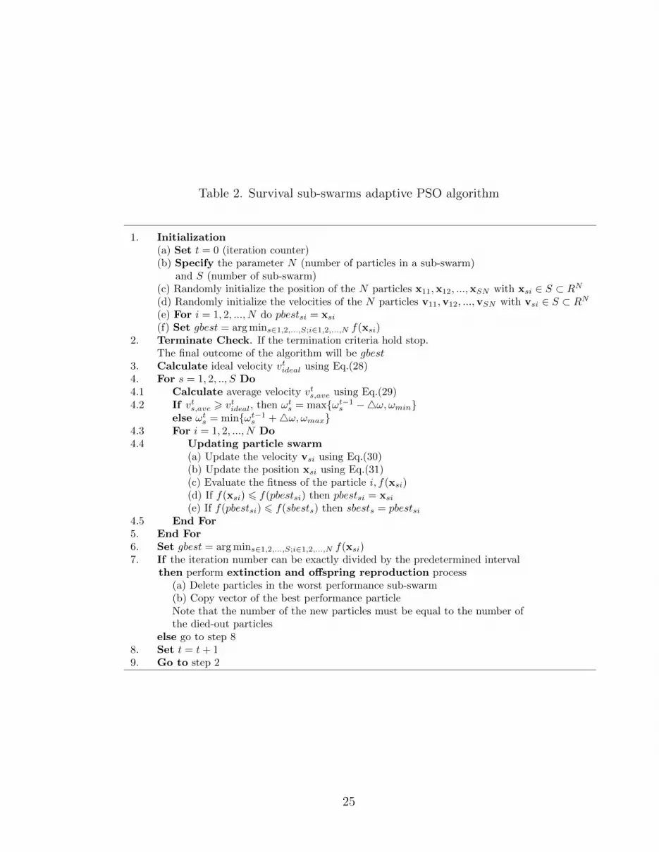
Table 2. Survival sub-swarms adaptive PSO algorithm

1. Initialization(a) Set t = 0 (iteration counter)(b) Specify the parameter N (number of particles in a sub-swarm)

and S (number of sub-swarm)(c) Randomly initialize the position of the N particles x11,x12, ...,xSN with xsi ∈ S ⊂ RN

(d) Randomly initialize the velocities of the N particles v11,v12, ...,vSN with vsi ∈ S ⊂ RN

(e) For i = 1, 2, ..., N do pbestsi = xsi

(f) Set gbest = arg mins∈1,2,...,S;i∈1,2,...,N f(xsi)2. Terminate Check. If the termination criteria hold stop.

The final outcome of the algorithm will be gbest3. Calculate ideal velocity vtideal using Eq.(28)4. For s = 1, 2, .., S Do4.1 Calculate average velocity vts,ave using Eq.(29)4.2 If vts,ave > vtideal, then ωt

s = max{ωt−1s −4ω, ωmin}

else ωts = min{ωt−1

s +4ω, ωmax}4.3 For i = 1, 2, ..., N Do4.4 Updating particle swarm

(a) Update the velocity vsi using Eq.(30)(b) Update the position xsi using Eq.(31)(c) Evaluate the fitness of the particle i, f(xsi)(d) If f(xsi) 6 f(pbestsi) then pbestsi = xsi

(e) If f(pbestsi) 6 f(sbests) then sbests = pbestsi4.5 End For5. End For6. Set gbest = arg mins∈1,2,...,S;i∈1,2,...,N f(xsi)7. If the iteration number can be exactly divided by the predetermined interval

then perform extinction and offspring reproduction process(a) Delete particles in the worst performance sub-swarm(b) Copy vector of the best performance particleNote that the number of the new particles must be equal to the number ofthe died-out particles

else go to step 88. Set t = t+ 19. Go to step 2

25

this behavior helps the whole swarm maintain its diversity. The swarm may benefit

from this phenomenon through more exploration of the search space [40, 41, 42, 43].

A simple velocity-line bouncing method is applied [40] to prevent a collision of

two particles from different sub-swarms by replacing Eq.(31) with Eq.(32) in which

the second and the third term are combined in an “OR” logical constraint. The

distance r1 is the dynamic criterion which is used to initiate the effectiveness of a

bounce-factor, δ. In other words, if the euclidean distance between two different

sub-swarm particles is less than r1, the bounce-factor shall alter the particle’s

velocity in order to avoid a collision. The equations of both position update and

r1 calculation are shown as:

xt+1sij = xtsij + τsiδv

t+1sij + (1− τsi)vt+1

sij (32)

where δ is the predetermined bounce-factor. This equation gives the particle the

possibility of making a U-turn and returning to where it came from (by setting

a negative bounce-factor). Particles can be slowed down (bounce-factor between

0 and 1) or sped up to avoid a collision (bounce-factor greater than 1). τsi is a

binary number which equals 1 when two particles from different sub-swarms are

close to other particles within distance r1, otherwise it is equal to 0.

r1 =T − tT×√D × (xmax − xmin)2

20(33)

where T is the maximum iteration, t is the current iteration, D is the dimension

of vectors, and xmax and xmin are the upper bound and lower bound of the search

space, respectively.

The proposed PSO 2—survival sub-swarms adaptive PSO with velocity-line

bouncing (SSS-APSO-vb)—is developed from the proposed PSO 1. A particle

collision avoidance with velocity-line bouncing is illustrated in Fig. 3 and the

algorithm is described in Table 8. It should be noted that SSS-APSO is a special

case of SSS-APSO-vb when δ = 1.

26

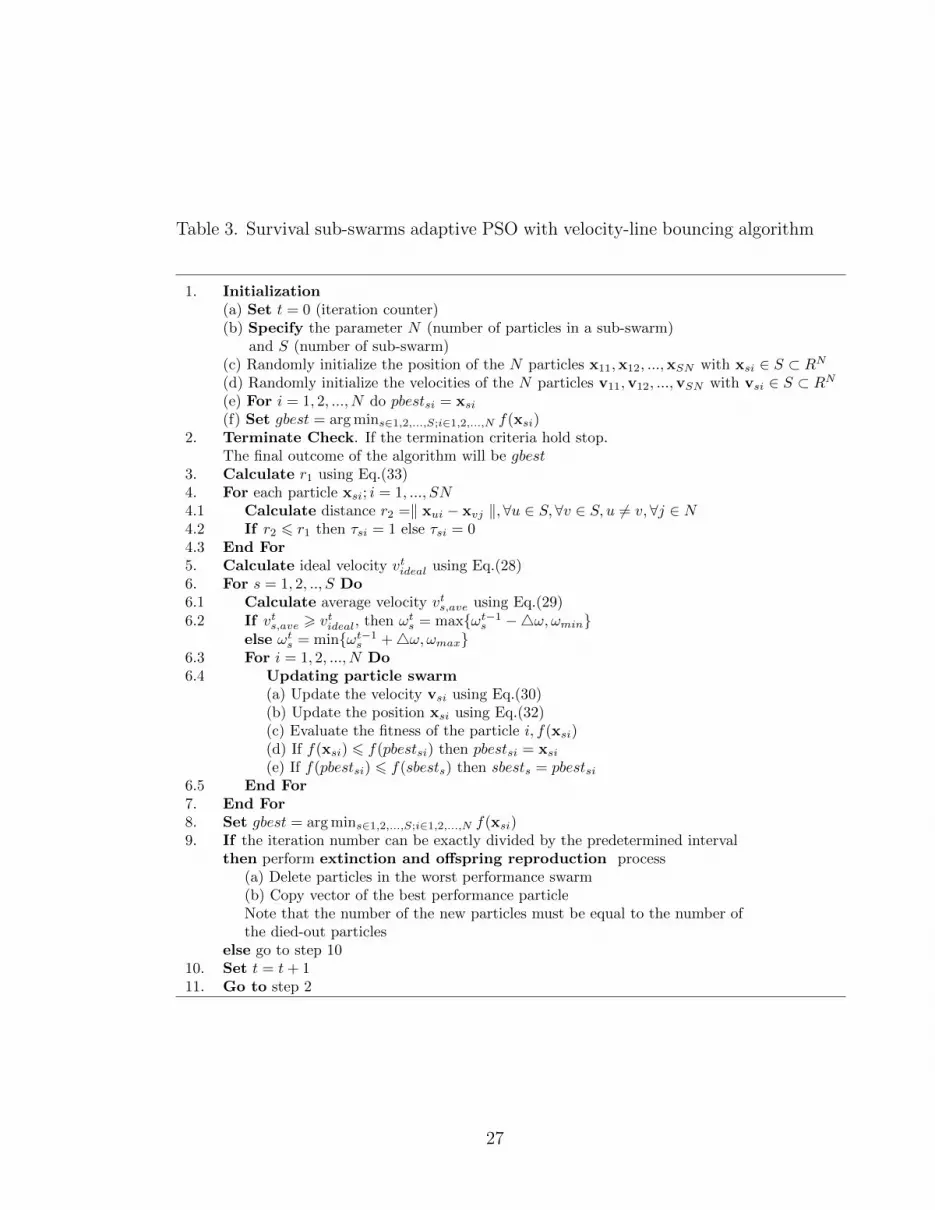
Table 3. Survival sub-swarms adaptive PSO with velocity-line bouncing algorithm


and S (number of sub-swarm)(c) Randomly initialize the position of the N particles x11,x12, ...,xSN with xsi ∈ S ⊂ RN

(d) Randomly initialize the velocities of the N particles v11,v12, ...,vSN with vsi ∈ S ⊂ RN


(f) Set gbest = arg mins∈1,2,...,S;i∈1,2,...,N f(xsi)2. Terminate Check. If the termination criteria hold stop.

The final outcome of the algorithm will be gbest3. Calculate r1 using Eq.(33)4. For each particle xsi; i = 1, ..., SN4.1 Calculate distance r2 =‖ xui − xvj ‖,∀u ∈ S, ∀v ∈ S, u 6= v,∀j ∈ N4.2 If r2 6 r1 then τsi = 1 else τsi = 04.3 End For5. Calculate ideal velocity vtideal using Eq.(28)6. For s = 1, 2, .., S Do6.1 Calculate average velocity vts,ave using Eq.(29)6.2 If vts,ave > vtideal, then ωt




(a) Update the velocity vsi using Eq.(30)(b) Update the position xsi using Eq.(32)(c) Evaluate the fitness of the particle i, f(xsi)(d) If f(xsi) 6 f(pbestsi) then pbestsi = xsi

(e) If f(pbestsi) 6 f(sbests) then sbests = pbestsi6.5 End For7. End For8. Set gbest = arg mins∈1,2,...,S;i∈1,2,...,N f(xsi)9. If the iteration number can be exactly divided by the predetermined interval

then perform extinction and offspring reproduction process(a) Delete particles in the worst performance swarm(b) Copy vector of the best performance particleNote that the number of the new particles must be equal to the number ofthe died-out particles


27

Figure 3. A particle-collision and the velocity-line bouncing

2.5 Numerical Experiments and Discussions

In order to demonstrate the effectiveness and performance of the proposed ap-

proaches, numerical experiments on eight nonlinear benchmark functions, which

consist of both unimodal and multimodal optimization problems have been per-

formed five other competitive algorithms for the comparison and have also been

implemented.

2.5.1 Benchmark functions

Three of the eight benchmark functions—Rosenbrock, Sphere, and Exponen-

tial functions—are unimodal landscape functions. The remaining functions are

multimodal landscape functions. All these problems are minimization problems.

The name, detailed description, and optimum solutions of theses functions are

shown in Table 4. It is worth mentioning that the Griewank function is a func-

tion with added noise. In low dimensions this function is a highly multi-modal

function, whereas in higher dimensions the Griewank function resembles a plain

Sphere-function, because the added noise diminishes (limD→∞∏D

i=1 cos(xi√i

)= 0

for randomly chosen xi).

28

Table 4. Benchmark Functions

Name Function Range x∗ f(x∗)

Rosenbrock f(x) =∑D−1

i=1

(100(xi+1 − x2i )2 + (xi − 1)2

)[−2.048, 2.048]D [1, ..., 1]D 0

Sphere f(x) =∑D

i=1 x2i [−100, 100]D [0, ..., 0]D 0

Exponential f(x) = − exp(−0.5

∑Di=1 x

2i

)[−1, 1]D [0, ..., 0]D −1

Griewank f(x) = 14000

∑Di=1 x

2i −

∏Di=1 cos

(xi√i

)+ 1 [−600, 600]D [0, ..., 0]D 0

Restringrin f(x) =∑D

i=1

(x2i − 10 cos(2πxi) + 10

)[−5.12, 5.12]D [0, ..., 0]D 0

2n Minima f(x) =∑D

i=1

(x4i − 16x2i + 5xi

)[−5, 5]D [−2.90, ...,−2.90]D −78.33D

Ackley f(x) = −20 exp(−0.2

√1D

∑Di=1 x

2i

)[−32.768, 32.768]D [0, ..., 0]D 0

− exp(

1D

∑Di=1 cos(2πxi)

)+ 20 + e

Schwefel f(x) = 418.9829D −∑D

i=1

(xi sin

√|xi|)

[−500, 500]D [420.9687, ..., 420.9687]D 0

Figure 4. Rosenbrock function

29

Figure 5. Sphere function

Figure 6. Exponential function

30

Figure 7. Restringin function

Figure 8. Ackley function

31

Figure 9. Schwefel function

2.5.2 Parameter settings

Five notable algorithms have been selected to be compared with the pro-

posed approaches. These algorithms were classic-PSO [2], LPSO [7], MPSO [15],

DAPSO [12], and APSO-VI [28]. The parameter settings of the different algo-

rithms are shown in Table 5. The experiments are conducted on dimensions of

5, 20, and 35 with the maximum number of function evaluations: 500, 1000, and

1500, respectively. The results of all experiments are averages taken from 40 inde-

pendent runs that were carried out to eliminate random discrepancy. The study

of Van den Bergh and Engelbrecht [44] showed that the effect of population size

on the performance of the PSO method is of little significance. Influenced by this,

all experiments in this study were conducted with a population size of 40.

Additionally, r in MPSO is the migratory rate of the sub-swarm. p in MPSO,

the proposed PSO 1, and the proposed PSO 2 is the number of sub-swarms. δ in

proposed PSO 2 is the bounce-factor.

32

Table 5. Parameter setting for comparison

Algorithm Parameters Setting References

classic-PSO ω = 0.729, φ1 = φ2 = 1.49 [2]LPSO ωmax = 0.9, ωmin = 0.4, φ1 = φ2 = 2.0 [7]MPSO ωmax = 0.9, ωmin = 0.4, φ1 = 2.5 to 0.5, φ2 = 0.5 to 2.5, [15]

p = 5, r = 0.4DAPSO ωini = 1.0, φ1 = φ2 = 2.0, α = 0.4, β = 0.8 [12]APSO-VI ωmax = 0.9, ωmin = 0.3,4ω = 0.1, φ1 = φ2 = 1.49 [28]Proposed PSO 1 ωmax = 0.7, ωmin = 0.2,4ω = 0.1, φ1 = φ2 = 2.0, p = 4 This researchProposed PSO 2 ωmax = 0.7, ωmin = 0.3,4ω = 0.1, φ1 = φ2 = 2.0, p = 4, This research

δ = 0.5

2.5.3 Results and analysis

All of the test results in terms of the mean final best value and its standard

deviation are summarized in Table 6 and Table 7. The best results among all

approaches are highlighted in boldface.

The Rosenbrock function is a unimodal landscape function. Its global op-

timum lies inside a long, narrow, parabolically-shaped flat valley, also known as

Rosenbrock’s valley. Finding the valley is trivial, converging to the global minimum

is difficult. As shown in Table 6, all of the approaches could not find the optimum

point. However, the proposed PSO 1 and the proposed PSO 2 outperformed the

other approaches by providing the best solutions on test functions with D = 20 and

D = 35 while MPSO provided the best solution on the test function with D = 5.

The Sphere and Exponential functions are not complicated landscapes. Most all

approaches provided the optimal solution for each problem size, but the proposed

PSO 1 (SSS-APSO) yielded the best solutions for 2 of the 3 test cases (dimensions

of 5, 20) with the Sphere function and yielded the global minimum solutions for 3

of the 3 test cases (dimensions of 5, 20, and 35) with the Exponential function.

33

Table 6. Mean fitness value and its standard deviation of different PSO algorithms on benchmark functions I

Proposed PSO 1 Proposed PSO 2Function Dimension classic-PSO LPSO MPSO DAPSO APSO-VI

(SSS-APSO) (SSS-APSO-vb)

Rosenbrock 5 1.01576 0.09686 0.07243 67.85008 0.27308 0.08107 0.20317(1.35632) (0.10853) (0.08860) (55.06996) (0.60603) (0.23919) (0.10947)

20 79.99163 38.69093 12.26108 60.15578 12.71504 4.02639 5.68190(208.68915) (134.03781) (20.95389) (130.83203) (19.13285) (4.22371) (15.10816)

35 2102.44964 1968.40725 802.46683 1478.47079 1456.80856 694.18444 621.61072(683.65060) (579.73949) (481.25325) (629.14297) (301.93744) (513.60348) (341.09365)

Sphere 5 0.00203 0 0 0 0.00003 0 0(0.01136) (0) (0) (0) (0.00007) (0) (0)

20 0.30763 0.01974 0.14296 0.10535 0.00011 0.00001 0.00001(1.41392) (0.12483) (0.78695) (0.66631) (0.00063) (0.00007) (0.00008)

35 500.01652 0.32435 0.40067 251.90321 0.00001 0.08336 0.10536(2207.21060) (0.16635) (0.22276) (1593.17578) (0.00006) (0.18232) (0.26037)

Exponential 5 -1 -1 -1 -1 -1 -1 -1(0) (0) (0) (0) (0) (0) (0)

20 -0.99776 -0.99999 -1 -0.95512 -1 -1 -0.99599(0.01335) (0) (0) (0.19810) (0) (0) (0.00739)

35 -0.79960 -0.89011 -0.99996 -0.43672 -0.90162 -1 -0.99846(0.25753) (0.13162) (0.00002) (0.49048) (0.17256) (0) (0.00972)

Griewank 5 1.48701 0.03489 0.03596 0.03911 0.05217 0.01455 0.06814(1.19274) (0.02895) (0.02201) (0.02838) (0.02684) (0.02566) (0.03632)

20 0.02717 0.03412 0.24963 0.16057 0.09401 0.02564 0.09202(0.03591) (0.01535) (0.29782) (0.18173) (0.19421) (0.04988) (0.40939)

35 0.50848 0.63062 0.27902 67.05722 0.07528 0.39546 0.44129(0.30969) (0.26334) (0.11977) (33.20842) (0.02249) (0.29813) (0.32270)

1The numbers in parentheses are standard deviation

34

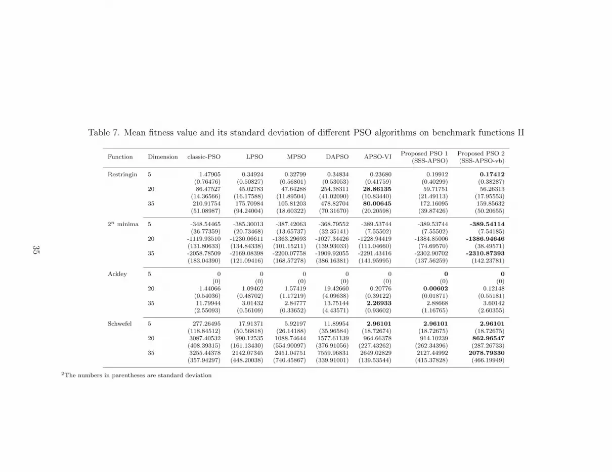
Table 7. Mean fitness value and its standard deviation of different PSO algorithms on benchmark functions II

Proposed PSO 1 Proposed PSO 2Function Dimension classic-PSO LPSO MPSO DAPSO APSO-VI

(SSS-APSO) (SSS-APSO-vb)

Restringin 5 1.47905 0.34924 0.32799 0.34834 0.23680 0.19912 0.17412(0.76476) (0.50827) (0.56801) (0.53053) (0.41759) (0.40299) (0.38287)

20 86.47527 45.02783 47.64288 254.38311 28.86135 59.71751 56.26313(14.36566) (16.17588) (11.89504) (41.02090) (10.83440) (21.49113) (17.95553)

35 210.91754 175.70984 105.81203 478.82704 80.00645 172.16095 159.85632(51.08987) (94.24004) (18.60322) (70.31670) (20.20598) (39.87426) (50.20655)

2n minima 5 -348.54465 -385.30013 -387.42063 -368.79552 -389.53744 -389.53744 -389.54114(36.77359) (20.73468) (13.65737) (32.35141) (7.55502) (7.55502) (7.54185)

20 -1119.93510 -1230.06611 -1363.29693 -1027.34426 -1228.94419 -1384.85006 -1386.94646(131.80633) (134.84338) (101.15211) (139.93033) (111.04660) (74.69570) (38.49571)

35 -2058.78509 -2169.08398 -2200.07758 -1909.92055 -2291.43416 -2302.90702 -2310.87393(183.04390) (121.09416) (168.57278) (386.16381) (141.95995) (137.56259) (142.23781)

Ackley 5 0 0 0 0 0 0 0(0) (0) (0) (0) (0) (0) (0)

20 1.44066 1.09462 1.57419 19.42660 0.20776 0.00602 0.12148(0.54036) (0.48702) (1.17219) (4.09638) (0.39122) (0.01871) (0.55181)

35 11.79944 3.01432 2.84777 13.75144 2.26933 2.88668 3.60142(2.55093) (0.56109) (0.33652) (4.43571) (0.93602) (1.16765) (2.60355)

Schwefel 5 277.26495 17.91371 5.92197 11.89954 2.96101 2.96101 2.96101(118.84512) (50.56818) (26.14188) (35.96584) (18.72674) (18.72675) (18.72675)

20 3087.40532 990.12535 1088.74644 1577.61139 964.66378 914.10239 862.96547(408.39315) (161.13430) (554.90097) (376.91056) (227.43262) (262.34396) (287.26733)

35 3255.44378 2142.07345 2451.04751 7559.96831 2649.02829 2127.44992 2078.79330(357.94297) (448.20038) (740.45867) (339.91001) (139.53544) (415.37828) (466.19949)

2The numbers in parentheses are standard deviation

35

In regards to the Griewank function, the algorithms presented do not perform

much better than the classic-PSO on dimensions of 20 and 35. A possible reason

for this is that the Griewank function is essentially unimodal when the dimension

is larger than the range of 10-15 (as mentioned before). Thus, the classic-PSO and

LPSO have no difficulty in finding the global optimum.

Optimizing the Restringin function presents a complex problem. Because it

is highly multimodal, an approach can easily become trapped in a local minimum

on its way to the global minimum. The APSO-VI performs better than the other

approaches on high dimension problems (e.g., 20 and 35).

The 2n minima function has some local minimum points and a relatively flat

bottom which includes the global minimum. The proposed PSO 2 provides the

best solutions in all higher dimension problems.

All approaches yield the global optimum solution on the Ackely function when

the dimension of the problem is 5. However, when the dimension increases to 35,

APSO-VI provides the better solution. The last benchmark function is the Schwefel

function. Its surface is comprised of a great number of peaks and valleys. The

function has a second best minimum, far from the global minimum, where many

search algorithms are trapped. Accordingly, the optimizers have a tendency to be

proned to convergence in the wrong direction in the optimization of the function.

As the results in Table 6 and Tabel 7 indicate, SSS-APSO and SSS-APSO-vb yield

better solutions when compared to the other approaches.

If we count the test problems as the combination of functions and the size of

the dimensions, we have 24 test cases. Proposed PSO 2 (SSS-APSO-vb) yields the

best solutions for 12 of the 24 test cases. Proposed PSO 1 (SSS-APSO) provides

the best solutions for 11 of the 24 test cases. However, APSO-VI, MPSO, DAPSO,

LPSO, and classic-PSO yield the best solutions for 9, 5, 3, 3, and 2 of the 24 test

36

cases, respectively.

Proposed PSO 1 (SSS-APSO) outperforms proposed PSO 2 (SSS-APSO-vb)

on unimodal functions by yielding the best solutions for 6 of the 9 test cases

(Rosenbrock, Spere, and Exponential functions) while proposed PSO 2 yields the

best solutions for 4 of the 9 test cases. However, proposed PSO 2 (SSS-APSO-vb)

beats proposed PSO 1 (SSS-APSO) on multimodal functions by provides the best

solutions for 8 of the 15 test cases while proposed PSO 1 provides the best solutions

for 5 of the 15 test cases. The results show that the velocity-line bouncing method

enhances the particles explore the search spaces effectively.

In the following sections, I shall discuss the characteristics of the proposed

PSOs compared to the previously reported approaches.

The characteristics of proposed algorithms

Fig. 10, Fig. 11, Fig. 12, and Fig. 13 illustrate the mean best fitness trend-

lines, averaged for 20 runs on the Rosenbrock, Sphere, 2n minima, and Schwefel

functions. The x axis is the iteration number and the y axis is the mean fitness

value of gbest which is the best position ever visited by all particles. Fig. 10

shows that the rate of convergence of the proposed PSOs is similar to the other

approaches.

For a simple landscape like the Sphere function, Fig. 11 shows that all opti-

mizers are similar in their convergence rates for finding the global optimum. Nev-

ertheless, the Particle Swarm shows quicker local and global search performance

when compared with other competitive algorithms.

The performance of new approaches is also better in multimodal test functions.

Fig. 12 shows that both the proposed PSO 1 and the proposed PSO 2 converge

to the optimum solution quickly, even faster than LPSO. Furthermore, they also

yield the best solution among other competitive algorithms while the classic-PSO,

37

Figure 10. Performance on Rosenbrock, D = 20, T = 1000

Figure 11. Performance on Sphere, D = 20, T = 1000

38

Figure 12. Performance on 2n minima, D = 20, T = 1000

LPSO, MPSO, and DAPSO all remain stuck at local minima.

The stagnation problem can be clearly observed in Fig. 13. The classic-PSO

and LPSO are trapped in local optima in early iteration (before 150th iteration)

while the proposed PSOs’ searches continue. Furthermore, we can see that both

the proposed PSOs yield the minimum solutions when compared with the other

optimizers. In conclusion, the ability to mitigate premature convergence of my

approaches is affirmed in the multimodal functions, Fig.12 and Fig. 13.

In summary, these new approaches work well on unimodal functions although

their convergence rates are not significantly different from other comparable algo-

rithms. For multimodal functions, the proposed PSOs are found to outperform

other competitive algorithms in that they exhibit the ability to avoid local optima.

In the next section, we shall discuss another parameter, diversification, which is

key factor of the proposed PSOs’ performance.

Diversification

As the results of the experiments demonstrate, the proposed algorithms appear

to be, for these functions, much stronger optimizers. They yielded the best solution

in highly multimodal problems such as 2n minima and Schwefel. One of the key

39

Figure 13. Performance on Schwefel, D = 20, T = 1000

factors of the results is the diversification. While the classic-PSO tends to converge

on a local optimum, the proposed methods overcome this limitation. The main

explanation of this performance is that the algorithms maintain a high diversity

throughout the run. Let us consider a common measure for the diversity called

the “distance-to-average-point”, defined by the following equation.

diversity(S) =1

|N |·|N |∑i=1

√√√√ D∑j=1

(xij − xj)2 (34)

where N is the population, |N | is the swarmsize, D is the dimensionality of the

problem, xij is the j’th value of the i’th particle, and xj is the j’th value of the

average point x.

Fig. 14 shows the diversity comparison among the classic-PSO, LPSO, and

the proposed PSO 2 on the Rosenbrock function. It is clear that the proposed PSO

2 maintains a high value of diversity as the evolution process proceeds while the

classic-PSO and LPSO reduce their diversity rapidly. It is worth noting that the

process of extinction and offspring reproduction systematically keeps the diversity

of the proposed PSOs reduced; the dramatic changes of the diversity at 250th, 500th

and 750th iteration demonstrate this.

Fig. 15 shows the diversity comparison among the MPSO, APSO-VI, and the

40

Figure 14. Diversity on Rosenbrock (I), D = 20, T = 1000

proposed PSO 2. Again, the proposed PSO 2 maintains its diversity better than

the others. Additionally, the diversity of the proposed algorithm reduces until it

is comparable to the APSO-VI. As we mentioned earlier, the proposed PSOs are

based on the APSO-VI. Therefore, the proposed PSO 2 acts like the APSO-VI

when the sub-swarms have been merged to the whole swarm.

Fig. 16 and Fig. 17 illustrate the diversity comparison among the classic-

PSO, LPSO, MPSO, APSO-VI, and the proposed PSO 2 on the Schwefel function.

Similarly, the proposed PSO 2 dominates the other algorithms with regards to

the diversity. This proves that the diversity of the new approaches is significantly

improved, and it is the reason why the proposed algorithms more frequently may

generate the satisfactory solutions.

2.6 Conclusions

In this chapter two novel self-adaptive particle swarm optimization algorithms,

called Survival Sub-swarms adaptive PSO (SSS-APSO) and Survival Sub-swarms

adaptive PSO with velocity-line bouncing (SSS-APSO-vb) have been developed.

These proposed algorithms mimic the behavior of swarms by encoding both social

and individual perspectives. From the social point of view, the whole swarm di-

41

Figure 15. Diversity on Rosenbrock (II), D = 20, T = 1000

Figure 16. Diversity on Schwefel (I), D = 20, T = 1000

Figure 17. Diversity on Schwefel (II), D = 20, T = 1000

42

vides into many sub-swarms and performs extinction and offspring reproduction

processes periodically. From the individual point of view, the particles maintain

space between each other in order to avoid a collision. The objective of these

methods is to mitigate a stagnation problem while the local search is maintained

by executing both the exploration and the exploitation stages of the iteration si-

multaneously.

The performance of the proposed algorithms is evaluated on well-known

benchmark functions. The results show that the SSS-APSO and the SSS-APSO-vb

not only frequently yield the best solutions—when compared to the other compet-

itive algorithms—but also converge to the optima relatively quickly. Specifically,

the SSS-APSO works well on the unimodal test functions while the SSS-APSO-vb

works well on the multimodal test functions.

43

List of References

[1] R. Eberhart and J. Kennedy, “A new optimizer using particle swarm theory,”in Proceedings of the Sixth Internation Symposium on Micro Machine andHuman Science, 1995, pp. 39–43.

[2] J. Kennedy and R. Eberhart, “Particle swarm optimization,” in Proceedings ofIEEE International Conference on Neural Networks IV, 1995, pp. 1942–1948.

[3] M. Clerc and J. Kennedy, “The particle swarm - explosion, stability, andconvergence in a multidimensional complex space,” IEEE Transactions onEvolutionary Computation, vol. 6(1), pp. 58–72, 2002.

[4] K. E. Parsopoulos and M. N. Vrahatis, Particle Swarm Optimization andIntelligence: Advances and Apllications, 1st. edn. Hershey, PA, USA: ISTELtd., 2010.

[5] R. C. Eberhart and Y. Shi, “Comparing inertia weights and constriction fac-tors in particle swarm optimization,” in Proceedings of the IEEE Congress onEvolution Computation, 2000, pp. 84–88.

[6] K. E. Parsopoulos and M. N. Vrahatis, “Unified particle swarm optimizationfor tackling operations research problems,” in Proceedings of swarm intelli-gence symposium SIS, 2005, pp. 53–59.

[7] Y. Shi and R. C. Eberhart, “A modified particle swarm optimizer,” in Pro-ceedings of the Evolutionary Computation, 1998, pp. 69–73.

[8] Y. Shi and R. C. Eberhart, “Empirical study of particle swarm optimization,”in Proceedings of the IEEE congress on Evolutionary Computation, 1999, pp.1945–1950.

[9] G. Ueno, K. Yasuda, and N. Iwasaki, “Robust adaptive particle swarm opti-mization,” in Proceedings of IEEE International Conference on System, Manand Cybernetics, 2005, pp. 3915–3020.

[10] T. J. Ai and V. Kachitvichyanukul, “A study on adaptive particle swarmoptimization for solving vehicle routing problem,” in Proceedings of the 9thAsia Pacific Industrial Engineering & Management Systems Conference, 2008,pp. 2262–2268.

[11] N. Iwasaki, K. Yasuda, and G. Ueno, “Dynamic parameter tuning of particleswarm optimization,” IEEJ Transactions on Electrical and Electronic Engi-neering, vol. 1, pp. 353–363, 2006.

[12] X. Yang, J. Yuan, J. Yuan, and H. Mao, “A modified particle swarm opti-mization with dynamic adaptation,” Applied Mathematics and Computation,vol. 189, pp. 1205–1213, 2007.

44

[13] K. Yasuda, N. Iwasaki, G. Ueno, and E. Aiyoshi, “Particle swarm optimiza-tion: a numerical stability analysis and parameter adjustment based on swarmactivity,” IEEJ Transactions on Electrical and Electronic Engineering, vol. 3,pp. 642–659, 2008.

[14] J. Liu, X. Ren, and H. Ma, “A new pso algorithm with random c/d switch-ings,” Applied Mathematics and Computation, vol. 218, pp. 9579–9593, 2012.

[15] M. Gang, Z. Wei, and C. Xiaolin, “A novel particle swarm optimization algo-rithm based on particle swarm migration,” Applied Mathematics and Compu-tation, vol. 218, pp. 6620–6626, 2012.

[16] A. Leontitsis, D. Kontogiorgos, and J. Pagge, “Repel the swarm to the opti-mum,” Applied Mathematics and Computation, vol. 173, pp. 265–272, 2006.

[17] B. Kaewkamnerdpong and P. J. Bentley, “Perceptive particle swarm optimiza-tion,” in Proceedings of the International Conference on Adaptive and NaturalComputing Algorithms, 2005, pp. 259–263.

[18] B. Kaewkamnerdpong and P. J. Bentley, “Perceptive particle swarm opti-mization: an investigate,” in Proceedings of 2005 IEEE on Swarm IntelligenceSymposium, 2005, pp. 169–176.

[19] S. Yang, M. Wang, and L. Jiao, “A quantum particle swarm optimization,”in Proceedings of the IEEE Congress on Evolutionary Computation, 2004, pp.320–324.

[20] M.-R. Chen, X. Li, X. Zhang, and Y.-Z. Lu, “A novel particle swarm optimizerhybridized with extremal optimization,” Applied Soft Computing, vol. 10, pp.367–373, 2010.

[21] W. Deng, R. Chen, B. He, Y. Lu, L. Yin, and J. Gup, “A novel two-stagehybrid swarm intelligence optimization algorithm and application,” Soft Com-puting, vol. 6(10), pp. 1707–1722, 2012.

[22] P. Shelokar, P. Siarry, V. Jaryaraman, and B. Kulkarni, “Particle swarm andant colony algorithms hybridized for improved continuous optimization,” Ap-plied Mathematics and Computation, vol. 188, pp. 129–142, 2007.

[23] H.-L. Shieh, C.-C. Kuo, and C.-M. Chiang, “Modified particle swarm opti-mization algorithm with simultated annealing behavior and its numerical ver-ification,” Applied Mathematics and Computation, vol. 218, pp. 4365–4383,2011.


45

[25] Y. Marinakis and M. Marinaki, “A hybrid multi-swarm particle optimizationalgorithm for the probabilistic traveling sales problem,” Computers & Opera-tions Research, vol. 37, pp. 432–442, 2010.

[26] Z. Xuanping, D. Yuping, Q. Guoqiang, and Q. Zheng, “Adaptive particleswarm algorithm with dynamically changing inertia weight,” Xi’an JiaotongUniversity, vol. 39, pp. 1039–1042, 2005.

[27] P. K. Tripathi, S. Bandyopadhyay, and S. K. Pal, “Multi-objective particleswarm optimization with time variant inertia and acceleration coefficients,”International Jouranl of Information Science, vol. 177, pp. 5033–5049, 2007.

[28] G. Xu, “An adaptive parameter tuning of particle swarm optimization al-gorithm,” Applied Mathematics and Computation, vol. 219, pp. 4560–4569,2013.

[29] M. Jaing, Y. Luo, and Y. Yang, “Stochastic convergence analysis and pa-rameter selection of the standard particle swarm optimization algorithm,”Information Processing Letters, vol. 102, pp. 8–16, 2007.

[30] A. Banks, J. Vincent, and C. Anyakoha, “A review of particle swarm opti-mization. part 1: background and development,” Natural Computing, vol. 6,pp. 467–484, 2007.

[31] A. Banks, J. Vincent, and C. Anyakoha, “A review of particle swarm opti-mization. part 2: hybridisation, combinatorial, multicriteria and constrainedoptimization, and indicative applications,” Natural Computing, vol. 7, pp.109–124, 2008.

[32] I. C. Trelea, “The particle swarm optimization algorithm: convergence anal-ysis and parameter selection,” Information Processing Letters, vol. 85, pp.317–325, 2003.

[33] K. Veeramachaneni, T. Peram, C. Mohan, and L. A. Osadciw, “Optimizationusing particle swarms with near neighbor,” in Proceedings of Genetic andEvolutionary Computation Conference, 2003, pp. 110–121.



[36] J. Kennedy, “Small worlds and mega-minds: effects of neighborhood topol-ogy on particle swarm performance,” in Proceedings of IEEE Congress onEvolutionary Computation, 1999, pp. 1931–1938.

46

[37] J. Kennedy and R. Mendes, “Population structure and particle swarm per-formance,” in Proceedings of IEEE Congress on Evolutionary Computation,2002, pp. 1671–1676.

[38] M. Melanie, An Introduction to Genetic Algorithms. Cambridge, Mas-sachusetts: MIT Press, 1999.

[39] C. W. Reynolds, “Flocks, heards, and schools: a distributed behavioralmodel,” in Proceedings of the 14th annual conference on Computer graphicsand interactive techniques, 1987, pp. 25–34.

[40] T. Krink, J. S. Vesterstrom, and J. Riget, “Particle swarm optimisation withspatial particle extension,” in Proceedings of IEEE Congress on EvolutionaryComputation, 2002, pp. 1474–1479.

[41] J. Riget and J. S. Vesterstrom, “A diversity-guided particle swarm optimizer-the arpso,” Aarhus C, Denmark, Tech. Rep. EVALife No.2002-02, 2002.

[42] M. Pant, T. Radha, and V. P. Singh, “A simple diversity guided particleswarm optimization,” in Proceedings of IEEE Congress on Evolutionary Com-putation, 2007, pp. 3294–3299.

[43] N. Nakagawa, A. Ishigame, and K. Yasuda, “Particle swarm optimization withvelocity control,” IEEJ Transactions on Electrical and Electronic Engineering,vol. 4, pp. 130–132, 2009.

[44] F. van den Bergh and A. P. Engelbrecht, “Effects of swarm size on coopera-tive particle swarm optimisers,” in Proceedings of Genetic and EvolutionaryComputation Conference, 2001, pp. 892–899.

47

CHAPTER 3

PSO for Solving CVRP

The Capacitated Vehicle Routing Problem (CVRP) was first introduced by

Dantzig and Ramser [1]. The problem can be defined by a graph G = (V,A)

where V = {v0, v1, ..., vn} is the vertex set and A = {(vi, vj) : i 6= j, vi, vj ∈ V } is

the arc set. Vertex v0 represents a depot at which m identical vehicles are based,

while the remaining vertices correspond to cities or customers. Moreover, each

city vi has a demand di and the total demand of any route may not exceed the

identical vehicle capacity Q. A matrix C = (cij) is defined on A. The coefficients

cij represent distances, travel costs or travel times. The number of vehicles can be

a given constant or a decision variable.

The CVRP is the problem of constructing m vehicle routes of minimum total

cost starting and ending at the depot, such that each customer is visited exactly

once by one vehicle, and satisfying some side constraints. In this study, only the

case in which all the customers correspond to deliveries is considered. There is a

single depot and the demands are deterministic, known in advance, and may not be

split. The CVRP is a basic vehicle routing problem, however, there are numerous

variants of it with relaxation and/or additional constraints such as time windows,

heterogeneous vehicles, backhauls, and simultaneous pick up and delivery. Toth

and Vigo [2] provided the broad reviews on CVRP and other variants of VRP.

The CVRP is a well known NP-hard problem, therefore various heuristic and

metaheuristic algorithms such as simulated annealing (Breedam [3], Chiang and

Russell [4]), genetic algorithm (Ren and Li [5]), tabu search (Gendreau et al. [6]),

ant colony (Bullnheimer et al. [7]), and neural network (Torki et al. [8]) have been

proposed by a number of researchers for decades. Zhang et al. [9] provided a com-

48

prehensive review on metaheuristic algorithms and their applications. However, to

the best my knowledge, the applications of the particle swarm optimization (PSO)

on CVRP are not readily available.

3.1 The Capacitated Vehicle Routing Problem (CVRP)3.1.1 The problem definition

I shall consider the static and deterministic version of the problem known as

the capacitated VRP (CVRP). The objective is to minimize the total cost (i.e., the

number of routes and/or their length or travel time) needed to serve all the cus-

tomers. Generally, the travel cost between the locations of each pair of customers

is the same in both directions (symmetric), whereas in some applications, where

there are one-way directions imposed on the roads, the travel cost between the

pair of customer locations is not the same in both directions (asymetric). Accord-

ingly, if the cost matrix of the problem is symmetric, the corresponding problem is

called symmetric CVRP (SCVRP). If the cost matrix of the problem is asymetric

(cij 6= cji), the corresponding problem is called asymetric CVRP (ACVRP).

The cost matrix satisfies the triangle inequality, cij 6 cik + ckj; ∀i, j, k ∈ V .

If there is such a case the instance does not satisfy the triangle inequality, the

equivalent instance may be obtained in an immediate way by adding a suitably

large positive quantity to the cost of each arc. It is possible, however, that this

operation affects the algorithm’s performance, resulting in poor solution quality

with respect to the original costs.

The graph G is assumed to be complete. It includes the arcs connecting all

the customer pairs. However, if G is not completely connected (but still strongly

connected), it is possible to obtain a complete graph in which the cost of each arc

(i, j) is defined as the cost of the shortest path from i to j. This method is referred

to as completely “triangularizing” a graph. Furthermore, if the instances that give

49

the coordinates of the vertices and the cost between a pair of customers—cij—can

be calculated, the instances are often called euclidean CVRP.

A set of m identical vehicles, each with capacity Q, is available at the depot.

Each vehicle performs at most one route. The m is not smaller than mmin, where

mmin is the minimum number of vehicles needed to serve all the customers. Usually,

the value of mmin can be determined by solving the bin packing problem (BPP).

Nonetheless, the mmin may be solved by the so-called continuous lower bound for

BPP: dd(S)/Qe. To ensure feasibility I assume that dj 6 Q for each j = 1, 2, . . . , n.

If m (number of available vehicles) is greater than mmin, it may be possible to

leave some vehicles unused. In such a case, fixed costs are often associated with the

use of the vehicles. In practical situations, the additional objective requiring the

minimization of the number of used vehicles is frequently present. The solver can

allow for the determination of the solutions using a number of vehicles smaller than

m by adding a large constant value to the cost of the arcs leaving the depot. In

contrast, if the solver determines only solutions using all the m available vehicles,

there are two possibilities. The first possibility is to compute mmin by solving the

BPP associated with CVRP, and then applying the algorithm with m = mmin.

The second possibility is to define an extended instance with a complete graph

G = (V , A) obtained from G by adding m−mmin dummy vertices to V , each with

demand dj = 0.

As mentioned before, the CVRP is known NP-hard problem, and generalizes

the well-known traveling salesman problem (TSP), arising when Q 6 d(V ) and

m = mmin = 1. Consequently, all the relaxations proposed for the traveling

salesman problem (TSP) are valid for the CVRP.

50

3.1.2 Problem formulation

As mentioned above, CVRP is defined as the problem of determining optimal

routes to be used by vehicles starting from a depot to serve all of the customers’

demands, observing some constraints. We can say that CVRP is the generalization

of VRP. The objective is to minimize travel cost, travel time, or the number of

vehicles depending on the problem goals. Furthermore, numerous vehicles are

available at the depot to serve customer demand and they must return to the

depot at the end of the operations. The CVRP is modeled as follows Kuo et al.

[10].

Notation

i, j Customer index; i = 1 . . . n, j = 1 . . . n

k Vehicle index; k = 1 . . .m

cij Distance between customer i and j

di Demand of customer i

Q Vehicle capacity

Decision variables

xijk =

{1 : if vehicle k passed route from i to j0 : otherwise

(35)

yik =

{1 : if customer i is visited by vehicle k0 : otherwise

(36)

51

Minm∑k=1

n∑j=0

n∑i=0

cijxijk (37)

Subject to,

n∑i=0

xi0k −n∑j=0

x0jk = 0, ∀k = 1, 2, . . . ,m (38)

n∑i=0

m∑k=1

xijk = 1, ∀j = 1, 2, . . . , n (39)

n∑j=0

m∑k=1

xijk = 1, ∀i = 1, 2, . . . , n (40)

n∑j=1

x0jk 6 1, ∀k = 1, 2, . . . ,m (41)

n∑i=0

xijk = yjk, ∀j = 0, 1, . . . , n; k = 1, 2, . . . ,m (42)

n∑j=0

xijk = yik, ∀i = 0, 1, . . . , n; k = 1, 2, . . . ,m (43)

n∑i=1

diyik 6 Q, ∀k = 1, 2, . . . ,m (44)

The objective of the function Eq.(37) is to minimize total travel distance,

while the constraint in Eq.(38) guarantees that the number of vehicles that arrives

at and departs from the depot is the same. Eq.(39) and Eq.(40) ensure that each

customer is visited exactly once. Eq.(41) defines how the available vehicle, m, can

be used. Eq.(42) and Eq.(43) show the relationship between two decision variables

(x, y). Eq.(44) guarantees that the vehicle capacity is not exceeded.

The algorithms for solving CVRP can be divided into two categories: exact

(mathematical-programming-based) and approximate (heuristic and metaheuristic)

algorithms.

3.1.3 Exact approaches

The exact algorithms can be also classified into three classes: direct tree

search method, dynamic programming, and integer linear programming [11]. La-

52

porte et al. [12] first proposed branch-and-bound algorithm for asymmetric CVRP

(ACVRP), a direct tree search method. By dropping the capacity-cut constraints

(CCCs) of two-index vehicle flow formulation, they solved the problem as an assign-

ment problem (AP), in which several efficient algorithms are available. Christofides

et al. [13] developed an algorithm for symmetric CVRP (SCVRP) which based on

the following k−degree center tree relaxation of the m-TSP; m is fixed. An ex-

tremely successful approach in solving optimal solutions of large instances CVRP

is branch-and-cut. However, the number of reports on branch-and-cut applied to

the CVRP is still limited, see Ralphs [14] for detailed survey. Set partitioning and

column generation fall into the third class, integer linear programming. Balinski

and Quandt [15] were among the first who proposed a set partitioning formulation

for VRP. However, there are two difficulties associated with the formulation: (i)

the large number of binary variable xj (exponential growth) in a real-life case, (ii)

the difficulty of computing cj values, see Toth [2] for the formulation. To over-

come theses difficulties, a column generation algorithm has been recommended by

a number of authors: Rao and Zionts [16], Desrosiers and Soumis [17], and Agarwal

et al. [18]. The application of column generation can be found in Desaulniers et

al. [19]. Nevertheless, the most successful exact algorithms for CVRP are branch-

and-cut-and-price approaches. These methods combine cut and column generation

with branch-and-bound. However, the algorithms typically need too much time

and memory for large instances. The largest problems which can be consistently

solved by the most effective exact algorithms proposed so far contain about 100

customers (within 16.67 hours) [2]. For more up-to-date review of the state-of-the-

art exact algorithms for the CVRP see Drexl [20], Ropke [21], and Baldacci et al.

[22].

53

3.1.4 Heuristic and metaheuristic approachesHeuristic approaches

Heuristic approaches can be divided into constructive procedures, and im-

provement procedures. The constructive procedures are used to compute the ini-

tial solutions (or the feasible initial solutions). The improvement procedures are

used to systemically improve the initial solutions.

The Clarke and Wright’s savings algorithm [23] is used to initialize the solu-

tions in which the number of vehicles is a decision variable. There are both parallel

and sequential versions of this algorithm. Laporte et at. [24] investigated the per-

formance of parallel saving algorithm and sequential saving algorithm. In their

study, the saving algorithm was combined with 3-opt exchange method [25] (an

improvement heuristic method) and the best improvement (BI) selection strategy

[26]. The experiment results showed that the parallel version outperformed the

sequential version.

The sweep algorithm (a constructive method) was proposed by Gillett and

Miller [27]. This algorithm uses the polar coordinates (θi, ρi) where θi is the angle

and ρi is the ray lenght of each customer i as the inputs. The algorithm starts

by arbitrarily assigning a customer i∗ value θ∗ = 0; then, computes the remaining

angles centered at 0 from the initial ray (0, i∗). Next, the customer is ranked

in increasing order of their θi. By doing this, the customers are clustered into

groups under the vehicle capacity constraint. Finally, each cluster is resolved by

a corresponding traveling salesman problem (TSP). There are also many other

constructive methods: Petal algorithms [15], Cluster-first-route-second algorithms

[28], Two-phase heuristic [29], etc. Toth and Vigo [2] and Laporte et al. [24]

provides details on these constructive algorithms.

As mentioned above, the improvement heuristics operate on the existing

routes. The improvement methods are categorized into “local improvement meth-

54

ods” and “global improvements methods”. The local improvement procedures find

a local minimum by performing moves and/or exchanges the customers in the sin-

gle route (intra-route improvement) and between two or more routes (inter-route

improvement). The search strategy is called “blind search heuristics” in which the

new solutions are generated based on the information gathered during the exe-

cution only [30]. These approaches are stopped when no further improvement is

found. This logic leads the local improvement methods to be trapped in a local

optimum. On the other hand, the global improvement methods temporarily accept

a worsening of the objective function value solutions. This strategy enhances the

possibility to leave the local optimum. The global improvement methods are often

called “metaheuristics”. The metaheuristic methods will be discussed in the next

section.

Lin [25] proposed the k -Opt exchange method for intra-route improvement.

The k edges are removed for the route and the k remaining segments are recon-

nected in all possible ways. If the lower objective function is found, the new route

configuration is accepted. The procedure stops if no further improvements can

be obtained. Verifying the k -Opt requires O(nk) time. Lin and Kernighan [31]

presented an extended version of the k -Opt method. In this new approach the

parameter k is dynamically modified throughout the search. Or [32] proposed

the Or-Opt exchange method. This improvement method selects a segment of l

of consecutive customers and relocates them into another place in a route. Ver-

ifying the Or-Opt exchange method requires O(n2) time. The 1-1 exchange, 1-0

exchange, CROSS exchange, GENI exchange, Descent heuristics are all inter-route

improvement methods which are based on exchange operations. Toth and Vigor[2],

Laporte et al. [24], Breedam [33], and Braysy and Gendreau [34] present additional

details.

55

Metaheuristic approaches

Metaheuristics are used to control the search processes performed by con-

structive and improvement heuristics. There are a number of reports which gave

a survey on metaheuristic approaches. Funk et al. [35] summarized the local

search methods. Ropke [21] discussed on the large neighborhood search methods.

Ahuja et al. [36] summarized the very large-scale neighborhood search methods.

Generally, the metaheuristics are divided into two categories: single-solution meta-

heuristics, where one agent is considered at a time, and population metaheuristics,

where multiple agents are considered concurrently [37]. Selected metaheuristic

methods: include simulated annealing, tabu search, genetic algorithm, and ant

colony optimization and are discussed here.

Simulated annealing (SA) was first introduced by Cerny [38] and Kirkpatrick

et al. [39]. Annealing denotes a process in which melted metal is cooled in order

to achieve a solid state of lower energy. If the cooling is done too fast, widespread

irregularities emerge in the structure of the solid, thus leading to relatively high-

energy states. On the other hand, a series of temperature levels is held long enough

at each level to reach equilibrium, leads to more regular structures associated with

low-energy states. In the context of optimization problems, a solution represents a

state of the physical system and the fitness value corresponds to the energy of the

system. At each iteration, the neighborhood solution is randomly selected from the

current solution. If the new solution yields an improvement, it is automatically

accepted as the new current solution. Otherwise, the new solution is accepted

upon the probability of acceptance. The probability of acceptance depends on the

magnitude of the fitness value increase and a parameter called the temperature.

Technically, at iteration t of the approach, a solution x is drawn randomly in N(xt).

If f(x) 6 f(xt), then xt+1 is set equal to x; otherwise, xt+1 = x with probability pt

56

or xt+1 = xt with probability 1 − pt. where pt = exp (− [f(x)− f(xt)] /θt) where

θt represents the temperature at iteration t. The temperature is reduced by the

cooling schedule. A number of cooling schedules has been proposed. One of the

common methods is a decreasing step function of t. At t = 1, we set θ1 > 0,

then the θt is multiplied by a factor α, (0 < α < 1) after every T iterations. The

implementation of simulated annealing to VRP can be found in Gengreau et al.

[40] and Cordeau et al. [41]

The principle of tabu search (TS) was proposed by Glover [42]. The idea be-

hind TS is to perform a local search where, at each iteration, the best fitness value

in the neighborhood of the current solution is selected as the new current solution,

even if it yields the worse fitness value. The approach will thus be able to escape

a local optimum. The tabu corresponds to a short-term memory in which stores

recently visited solutions to avoid short-term cycling. Tabu search’s application

on VRP can be found in [40]. One of the best TS algorithm in term of accu-

racy is Taillard’s algorithm [43]. This algorithm contains some of the features of

Taburoute [6]. Since Taillard’s algorithm uses standard insertion instead of a gen-

eralized insertion as in Taburoute, Taillard’s algorithm is simpler than Taburoute,

but managing the dynamic decomposition process, as well as the parallel imple-

mentation, adds to its complexity. There are a number of TS-based approaches;

granular tabu search algorithm by Toth and Vigo [44], adaptive memory tabu

search algorithm by Rochat and Taillard [45], unified tabu search algorithm by

Cordeau et al. [46], etc.

Genetic algorithms (GA) are in the class of the population metaheuristics.

The GA was first introduced by Holland [47]. This approach is motivated by

the way species evolve and adapt to their environment. It is started by encoding

the problem to produce a list of genes. The genes are then randomly combined to

57

produce a population of chromosomes, each of which represents a possible solution.

Genetic operations are performed on chromosomes that are randomly selected from

the population. This produces offspring. The fitness of these chromosomes is then

measured and the probability of their survival is determined by their fitness. The

detail description of GA can be found in Gen and Chen [48]. The genetic algorithm

had been widely applied to combinatorial optimization problems [37]. The broad

review of its applications to the VRP can be found in Toth and Vigo [2]. A

specific review of GA’s applications to the CVRP can be found in Laporte et al.

[24], Gendreau et al. [40], Baker and Ayechew [49].

The original Ant system framework was first described by Colorni et al. [50].

It is well known that ants can manage to find shortest paths from their nest to

food sources. A chemical compound—pheromone—is used to communicate among

the ants, which is laid down along the path. In the beginning, ants perform a

random search around their nest for food. As soon as a food source is found, they

bring it back to the nest and the pheromone is laid on the ground simultaneously.

Due to the frequent passage of ants and pheromone evaporation, the shortest path

between the nest and the food source tends to be accumulate more pheromone than

the rest paths. Therefore, an ant starting its route from the nest will be strongly

stimulated by higher pheromone level and follow the shortest path to the food

source. This is an efficient method to solve a shortest-path problem. Ant Colony

Optimization (ACO) emulates this natural mechanism. Artificial ants start from

an initial search point and sequentially build the components of a new potential

solution. A probabilistic decision is made among alternatives of each component. A

pheromone level at each alternative is used to determined its selection probability.

After the selection, each selected alternative is updated at the end of the tour, based

on the quality of the obtained solution. Thus, the components of solutions with

58

low function values are assigned higher pheromone levels. Additionally, in order to

avoid a local optimum, pheromone evaporation also take place. Colorni et al. [50]

illustrated the basic principles of ACO by applying to traveling salesman problem

(TSP). Dorigo and Stutzle [51] provided the review of ACO and its variants. The

application of ACO to solve VRP can be found in Bullnheimer et al. [7], Kawamura

et al. [52], and Bullnheimer et al. [53].

3.2 Discrete Particle Swarm Optimization

Since the CVRP is a discrete domain optimization problem, we need to un-

derstand discrete PSO version as well. This section discusses the PSO in discrete

domain problems.

The discrete binary PSO was first introduced by Kennedy and Eberhart [54].

In the binary PSO version, each particle represents its position in binary values

either 0 or 1; the particle’s personal best and the global best is still updated as

in the continuous version which is described in Eq.(45). However, the speed of

the particles need to be constrained to the interval [0, 1]. Thus, a logistic trans-

formation can be used to transform the real number to the binary number. The

normalization function used in is a sigmoid function as in Eq.(46). Then, the new

position of the particles is obtained as Eq.(47).

vtij = ωvt−1ij + φ1β1(pbestt−1ij − xt−1ij ) + φ2β2(gbest

t−1j − xt−1ij ) (45)

vtij = sig(vtij) =1

1 + e−vtij

(46)

xt+1ij =

{1 : if rij < vt+1

ij

0 : otherwise(47)

where rij is a uniform random number in the range [0, 1].

The limitation of the velocity is a problem. vtij should not approach too close

to 0.0 or 1.0. This ensures that there is always some chance of a bit flipping. Thus,

a constant parameter Vmax can be set at the start of a trial to limit the range of

59

vij. In practice Vmax is often set at ±4.0. Accordingly, with vij ≈ 0.017986, there

is always a chance of that a bit will change state. Kennedy and Eberhart named

this concept “the change of change” [54]. Also see Kennedy and Eberhart [55], and

Osadciw and Veeramachaneni [56] for more discussion on this topic. In conclusion,

the discrete binary PSO can update the particles positions in two steps. First,

Eq.(45) is used to update the velocity of the particle and the sigmoid function,

Eq.(46), is used to transform the velocity to [0, 1] scale. Second, the new position

of the particles are calculated using Eq.(47), [57].

There are other discrete PSO techniques. Al-kazemi and Mohan [58] used

the discrete binary PSO based technique which had particles alternatively exploit

personal best and neighborhood best positions instead of simultaneously. In a

subsequent Al-kazemi paper [59], he extended his former study by proposing a

new schematic which able to solve both discrete and continuous problems. Yang

et al. [60] developed an algorithm based on discrete binary PSO which uses a

different method to update velocity.

Khanesar et al. [61] pointed two main problems of the discrete binary PSO.

Firstly, it is not easy to select the value of inertia weight, ω. Secondly, the updating

position as in Eq.(47) is independent from the current position of that bit. The

value is solely updated using the velocity vector. This is much different from the

continuous PSO; where the update rule uses the current position of the swarm

and the velocity vector just determines the movement of the particle in the space.

Therefore, Khanesar et al. [61] proposed a new binary PSO which is choosing the

proper value for ω is solved. The previous direction and previous state of each

particle is also taken into account. The test results of the new method showed

that the new approach returned quite satisfactory results in number of the test

problems.

60

There are many papers that discuss the application of the binary discrete PSO.

Clerc [62] applied the discrete PSO with the traveling salesman problem (TSP).

The report claimed that the binary discrete PSO is not as powerful as some specific

algorithms. Zhong et al. [63] also studied the application of the binary discrete

PSO for solving the TSP. They introduced a new parameter, c3, as the mutation

factor. The new parameter helps the algorithm keeps the balance between the

exploration and the exploitation. It was proved that the mutation factor affects

the performance of the discrete PSO. Pang et al. [64] introduced a fuzzy matrix

in order to represent TSP solution. This study reported that even though the

fuzzy discrete PSO was not dominate Lin-Kernigham algorithm [31]; however, the

study showed the idea of solving the combinatorial optimization problems using the

particle swarm optimization. Ponnambalam et al. [65] solved a flowshop scheduling

problem by the discrete PSO. The objective function of this problem was a multi-

objective function in which the pareto optimal set and non-dominated solutions

concepts were considered. Tsai and Wu [57] deployed the binary discrete PSO for

solving the feeder reconfiguration problems in a power distribution system. The

sigmoid function was used to transform the real number of velocity to the interval

[0, 1] as explained above. The experimental results of the study claimed that the

binary PSO could solve the feeder configuration problems effectively. However,

the authors pointed out that the parameter selection such as inertia weight and

acceleration constants is also problematic.

There are papers discussed multi-valued discrete PSO. Pugh and Martinoli

[66] presented an idea of the transformation method for multi-value discrete PSO.

The particle representation of their method goes from being 2-dimensional to 3-

dimensional: xijk is a continuous real-value indicator of the probability of particle

i, element j assuming integer value k. Accordingly, to generate a value from 0 to

61

n, I must transform the real-valued terms xij0, . . . , xijn. The sigmoid function is

applied to each term, and use the weighted sum as the probability, are shown as:

x′ij =n∑k=0

vtijk (48)

Prob(xij = k) =vtijkx′ij

(49)

where x′ij is the normalizing coefficient for particle i, element j. By using this

technique, the particle can potentially generate any possible solution, but with

varying probabilities depending on its terms.

Osadciw and Veeramachaneni [56] summarized the multi-valued discrete PSO

technique. For the discrete optimization problem, the range of variables lie between

0 and Z−1 (Z is a non-negative integer). Eq.(45) is also used in this case. However,

the position update equation is changed as follows.

vtij = sig(vtij) =Z

1 + e−vtij

(50)

xt+1ij = round(vtij + (Z − 1)× σ × β) (51)

xt+1ij =

{Z − 1 : if xt+1

ij > Z − 10 : if xt+1

ij < 0(52)

Eq.(50) transforms the velocity to the continuous value between 0 and Z.

Eq.(51) generates a discrete number between 0 and Z− 1 using a normal distribu-

tion with µ = sig(vtij) and σ as parameters (β is a random number, [0, 1]). The

number is rounded to the closest discrete variable with the end points fixed by

Eq.(52). The velocity update equation remains the same as the continuous PSO.

The positions of the particles are discrete values between 0 and Z − 1. For any

given sig(vtij), we have an associated probability for any number between [0, Z−1].

Nevertheless, the probability of drawing a number randomly reduces based on its

distance from sig(vtij).

Based on the probability method (sigmoid function transformation), a particle

can assume different element values on different evaluations and therefore return

62

different fitness values. This problem may be called a noisy fitness problem. Pugh

and Martinoli [66] dealt with the noisy fitness problem by applying the technique

in Pugh et al. [67]. The noise-resistant PSO technique of Pugh et al. was inspired

by the modification of genetic algorithm (GA) which presented by Antonsson et al

[68]. The technique reevaluates the previous best particles at each iteration of the

algorithm and average all the evaluation results over the particles’ lifetimes to get

an average fitness. This technique is called the “aggregation function”.

Ps(µ) = (1

n

n∑i=1

µsi )1s (53)

where µi is the performance values over n evaluations, and s is the degree of

compensation. s determines how much weight is given to high-performing values

versus low-performing values.

P−∞ = lims→−∞

Ps = min (µ) (54)

P∞ = lims→∞

Ps = max (µ) (55)

P1 = avg(µ) (56)

Eq.(54) shows that if s closes to −∞, the value of P tends to the low-

performing values. On the other hand, Eq.(55) shows that if s approaches to

∞, the value of P tends to the high-performing values. Certainly, Eq.(56) shows

that if s = 1, P is the average of µ.

There are a small number of studies dealing with noisy fitness evaluation of the

evolutionary algorithms. Fitzpatrick and Grefenstette [69] investigated the trade

off between the population size and/or number of generations and the accuracy of

the function evaluations of a genetic algorithm in noisy environments. The authors

found that the genetic algorithms needs to sacrifice the accuracy of evaluations in a

noisy environment. Beyer [70] showed that the noise is the cause of the decreasing

convergence velocity and a residual location error in the final solution. From these

63

two papers, we find that the noisy fitness evaluation does not only deteriorate the

convergence velocity but also the accuracy. There is no a rule of thumb to deal

with the noisy fitness evaluation. Furthermore, most of the proposed methods are

the trade off between the convergence rate and computational time.

3.3 Particle Swarm Optimization for CVRP

This section reviews the literature regarding to the application of the PSO to

the vehicle routing problem. The VRP is a combinatorial optimization problem,

and the PSO was invented for the continuous domain problems. Some researchers

have proposed the PSO for solving the VRP. Chen et al. [71] adopt the quantum

discrete PSO algorithm to solve the capacitated VRP. The PSO is still used to

update the velocity and the position of the particles even though this algorithm

is the discrete version. Their algorithm also incorporates the simulated annealing

operator in which the new position of the particle is accepted with some probability.

The authors concluded that their new approach dominates the other heuristic

methods such as the genetic algorithm and simulated annealing.

Ai and Kachitvichyanukul [72] proposed the continuous PSO (the general

linear PSO) to solve the vehicle routing problem with simultaneous pickup and

delivery (VRPSD). The solution representation is a (n+ 2m)-dimensional particle

in which n is the number of customers and m is the number of vehicles. The first

n dimension represents the customer priority list and the following 2m dimension

represents the vehicle orientation. Their method starts with positioning the vehicle

orientations and then uses an insertion heuristics method to construct the routes.

The 2-opt algorithm is included in their method in order to improve the existent

routes. Finally, the authors proposed a special algorithm to reduce the required

vehicles. The experiment’s study showed that this approach is effective for solving

VRPSD. However, there are possible improvements such as the parameter settings,

64

the PSO algorithm implementation, or the local improvement heuristics.

Ai and Kachitvichyanukul [73] also introduced another idea for the solution

representation for the CVRP. The solution representation is a 3m-dimensional

particle in which m is the number of vehicles. The first two bits are the vehicle

orientation, and the last bit is the vehicle coverage radius. This approach starts

with positioning the vehicle orientations and assigning the vehicle coverage radius.

Then, a pragmatic algorithm is used to assign the customers to each vehicle orien-

tation. The 2-opt, 1-1 exchange, and 1-0 exchange are used to improve the existing

routes. The authors claimed that the new solution representation yielded a better

solution than the other approaches. However, the computation time of the new

approach is longer than that of their first approach, 48% on average (the approach

in [72]).

Kim and Son [74] introduced a probability-matrix-based solution representa-

tion for solving the CVRP. The principal of the matrix is the same as the from-

to-chart matrix. However, the range of the numbers in the matrix are the real

number between 0 to 1. The updating mechanism of the matrix is the typical PSO

method. However, their approach excludes the velocity updating. The particles’

position updating method can be shown as:

At+1i = wt1A

ti + wt2P

ti + wt3G

t (57)

where wt1 + wt2 + wt3 = 1, Ati is the matrix of the particle’s current position, P ti is

the personal best of the particle, and Gt is the global best of the swarm. t is the

iteration index (t = 1, 2, . . . , T ), and i is the particle index (i = 1, 2, . . . , N).

The inter-route improvement procedures (the 1-1 exchange and the 1-0 ex-

change) and the intra-route improvement procedures (2-opt and Or-opt) are used

to improve the existent routes. The authors claimed that based on the compu-

tational results, their approach outperformed Chen’s algorithm [71] and Ai and

65

Kachitvichyanukul’s algorithms [72, 73] on both the solutions’ quality and com-

putation time. However, as the matrix is a probability matrix, the different route

construction can be obtained from the identical matrix.

Kuo et al. [10] solved the CVRP with fuzzy demand by a hybrid PSO-GA

algorithm. Norouzi et al. [75] presented the multi-objective competitive open

vehicle routing problem in which the demand of each customer depends on the

reaching time and the vehicles do not need to start and finish at the same depot.

Marinakis et al. [76] applied the PSO on the CVRP with stochastic demands.

Belmecheri [77] solved the CVRP with heterogeneous fleet, mixed backhauls, and

time windows with the PSO. However, I shall focus on the conventional CVRP,

which I have defined the problem as in Section 3.1.1.

3.4 Proposed PSO for CVRP3.4.1 The framework

Two approaches to the PSO—the continuous PSO and the discrete PSO are

proposed. Both approaches share the common procedure shown in Fig. 18. The

first step is to generate an initial solution. To do this, a sweep algorithm [27] is

used to create the initial vehicle routes. The second step is the encoding method

which transforms this initial solution into arrays. There are significant differences

in this encoding method between the continuous PSO and the discrete PSO. This is

described in detail in Section 3.4.3 and Section 3.4.4. The third step calculates and

stores the best position (local best and global best) in memory. The fourth step is

the proposed PSO (SSS-APSO-vb) which enhances the global search performance

of the conventional PSO. This proposed PSO was described in Chapter 2. After

the particles are updated in step four, the fifth step decodes the arrays into routes

orientation. Next, the local improvement methods are applied: 2-Opt, Or-Opt,

1-1, and 1-0. These improvements methods are detailed in Section 3.4.5. In the

66

Figure 18. The proposed PSO procedure

seventh step, the local best and global best are updated with the results of step six.

The final step checks the stopping criteria. The proposed algorithm is described

in Table 8.

3.4.2 Initial solutions

The sweep algorithm, proposed by Gillett and Miller [27], is used to generate

the initial solution. This algorithm starts with randomly selecting a customer k.

Then it calculates the polar angle between the depot and the customer k. Next, it

calculates the polar angle of each customer in the customer set. Then it subtracts

the polar angle of each customer by the polar angle of k. After that, a sorting of

the customers in increasing order of new polar angle takes place. The smallest new

polar angle (the first customer in the sorted list) is assigned to the route; then the

next customer in the list is inserted if the capacity of the route is not exceeded.

67

Table 8. Survival sub-swarms adaptive PSO with velocity-line bouncing algorithm(for solving CVRP)


and S (number of sub-swarm)(c) Using the sweep algorithm to generate N initial solutions(d) Randomly initialize the velocities of the N particles v11,v12, ...,vSN

with vsi ∈ S ⊂ RN


(f) Set gbest = arg mins∈1,2,...,S;i∈1,2,...,N f(xsi)(g) Encode the N solutions to the N particles x11,x12, ...,xSN with xsi ∈ S ⊂ RN

2. Terminate Check. If the termination criteria hold stop.The final outcome of the algorithm will be gbest

3. Calculate r1 using Eq.(33)4. For each particle xsi; i = 1, ..., SN4.1 Calculate distance r2 =‖ xui − xvj ‖,∀u ∈ S, ∀v ∈ S, u 6= v,∀j ∈ N4.2 If r2 6 r1 then τsi = 1 else τsi = 04.3 End For5. Calculate ideal velocity vtideal using Eq.(28)6. For s = 1, 2, .., S Do6.1 Calculate average velocity vts,ave using Eq.(29)6.2 If vts,ave > vtideal, then ωt




(a) Update the velocity vsi; using Eq.(30) for the continuous PSO,using Eq.(30) and Eq.(50) for the discrete PSO

(b) Update the position xsi; using Eq.(32) for the continuous PSO,using Eq.(51) and Eq.(52) for the discrete PSO

(c) Decode the particle i to the solution i(d) Evaluate the fitness of the particle i, f(xsi)(e) Execute the integrated local improvement algorithms

with A = B = C = D = 30 (for this study)(f) If f(xsi) 6 f(pbestsi) then pbestsi = xsi

(g) If f(pbestsi) 6 f(sbests) then sbests = pbestsi6.5 End For7. End For8. Set gbest = arg mins∈1,2,...,S;i∈1,2,...,N f(xsi)9. If the iteration number can be exactly divided by the predetermined interval

then perform extinction and offspring reproduction process(a) Delete particles in the worst performance swarm(b) Copy vector of the best performance particleNote that the number of the new particles must be equal to the numberof the died-out particles


68

Table 9. The sweep algorithm

1. Arbitrary select a customer; k.2. Calculate the polar angle between the depot and the customer k

and set θ∗k = the polar angle of k.3. Calculate the polar angle between each customer and the depot, θi.4. Calculate θ∗i = θi − θ∗k5. Sort customers in increasing order of polar angle, θ∗i

(counter-clockwise direction):v1, v2, v3, . . . , vn.6. Start a new route6.1 Assign the first unrouted customer from the list to the route.6.2 Continue to assign the next customer on the list as long as

the route’s capacity is not exceeded.7. If the sorted list is not empty, go to step 4. Elese go to step 6.8. Execute local improvement procedure (as shown in section 3.4.5)

Figure 19. Solution representation (continuous)

This process is repeated until the sorted list of customers is empty. The detail of

the sweep algorithm is shown in Table 9.

One execution of the sweep algorithm yields one solution. Consequently, this

initial step is repeatedly executed until the number of solutions equals the number

of particles.

3.4.3 Continuous PSO

Solution representation of the vehicle routes is one of the key element when

implementing the PSO for CVRP effectively [72]. I use an array where each element

of the array is a continuous number between [0, n], where n is the number of

customers. Accordingly, the solution representation for a CVRP with n customers

is an n-dimensional particle. Fig. 19 shows a particle with 5 customers. Each

element in the particle is a continuous number between 0 and 5.

69

Figure 20. Encoding method (continuous version)

Encoding method (continuous version)

The initial solution must be encoded into array form in order to apply the PSO

algorithm. I propose a straightforward encoding method which considers the value

of the each array element as a priority number. An example of encoding the initial

solution is shown in Fig. 20. Since there are two routes in the initial solution, I

select the route which contains customer 1 to begin encoding. From the figure,

the route of (4, 1, 2, 5) is selected, and it is encoded by incrementally assigning

integer values from 1 to n. to the corresponding array elements. Accordingly, the

fourth element of the array is assigned the integer value “1”, the first element of

the array is assigned the value “2”, the second element of the array is assigned the

value “3” and so on. After integers are assigned to all customers in the first route

of Fig. 20, the second route is encoded. For this route, we do not assign number

“1” to the first customer in this route. Instead I continue where I left off on the

first route. As shown in Fig. 20, the sixth element of the array is assigned the

value “5”, and the third array element is assigned the value “6”.

Decoding method (continuous version)

The PSO solution is in array form, therefore I need to decode this array in or-

der to understand the route orientation of the solution. For example, given an array

70

Figure 21. Decoding method (continuous version)

Figure 22. Solution representation (discrete)

solution in Fig. 21, the route orientation is found by arranging the array indices by

sorting their corresponding element values in increasing order, (6 5 2 1 4 3). Since

the sixth element of the array has the smallest value, customer 6 is positioned first

in the route, followed by customer 5. When adding customers to the route, I must

determine if the customer can be added to the current route without violating

the vehicle capacity constraint. If, by adding the customer, the vehicle’s that the

second route is constructed after customer 5 is visited, because adding customer

2 immediately after customer 5 would violate the capacity constraint. Therefore,

customer 5 is followed by the depot, and customer 2 is the first customer on the

second route of the solution.

3.4.4 Discrete PSO

I make use of the multi-valued discrete PSO approach as shown in Eq.(50),

Eq.(51), and Eq.(52). The n-dimensional array represents the n-dimensional par-

ticle where n is the number of customers as the solution representation in the

71

Figure 23. A solution decoding I (discrete)

continuous PSO. However, the number in each element of the array is an integer

number which is [0, n− 1]. Fig. 22 shows a particle with 5 customers. As a result,

each element in the array is a discrete number between 0 to 4.

Encoding method (discrete version)

The encoding method is a straightforward encoding method as in Section

3.4.3. The solution diagram in Fig. 20 can be encoded to the n-dimensional array,

[1 2 5 0 3 4].

Decoding method (discrete version)

The decoding method of the discrete PSO is more complicated than that of

the continuous version. As previous stated, the position vector of a particle is the

integer numbers between [0, n− 1]. However, the velocity vector of the particle is

the continuous number between [−4.0, 4.0]. The bound assures, with a probability

of vij ≈ 0.017986, that the possibility that the bits will change state is maintained

[61]. I shall demonstrate the decoding method with Fig. 23 and Fig. 24 as an

example.

Suppose the top array in Fig. 23 is the velocity array (vij) of a problem with

6 customers. It is clear that the velocity of each dimension is a continuous number

between [−4, 4]. The bottom array in Fig. 23 shows the transformation of the

72

Figure 24. A solution decoding II (discrete)

velocity vector by Eq. (50) with Z = 6 (Z = n, for this study). Suppose we set

σ = 0.5, by using Eq. (51) and Eq. (52), we receive the particle’s position vector

(xt+1ij ) as in Fig. 24.

The array is sorted in increasing order, however due to the rounding in Eq.

(51), it is possible for multiple elements to have the same value as shown in Fig.

24. In this example, the second, fourth, and sixth elements are all assigned the

number “5”. Therefore, I shall use the sigmoid values as the sub-priority numbers.

The route construction is the same as described in Section 3.4.3. Therefore, sorting

the second, fourth, and sixth elements by increasing sigmoid value, the route for

this soluiton is 3-1-5-6-2-4.

The noise controlling

As previous stated, the noisy fitness problem is the issue of the discrete PSO

in which based on probability method. There are the noise-resistant methods in

other evolutionary methods and/or heuristic methods. However, it is rare in the

discrete PSO approach. By the way, the technique I selected has a parameter in

which able to control the noise in the step of changing from the velocity array to

the position array. The σ is a parameter which is required to be determined. The

large sigma value means the large noise. On the other hand, the small sigma value

73

Figure 25. The probabilities of different digits

means the small noise in the transformation process. The idea of sigma value can

be described as Fig. 25. The figure represents the transformation process of the

first element of the array (the sigmoid transformation) in Fig. 23. The mean of

this element is 1.37 (µ = 1.37) with σ = 0.5. As in Fig. 25, the area under the

curve between [−0.5, 0.5] is 0.04084, between [0.5, 1.5] is 0.56164, between [1.5, 2.5]

is 0.38552, and between [2.5, 3.5] is 0.01181.

Accordingly, the probability that the first element is assigned number “0”

is 4.084%, number “1” is 56.164%, number “2” is 38.552%, and number “3” is

1.181%. The other numbers ((−∞, 0] and [3,+∞)) will be assigned to the first

array with probability 0.019%. Technically, I can adjust these probabilities by

changing the value of σ. The larger sigma affects to the larger variation. On the

other hand, the smaller sigma affects to the smaller variation. Therefore, the noise

of the transformation process is controlled by the sigma value. See appendix B.

74

Figure 26. 2-opt exchange method

3.4.5 Local improvement

A number of local improvements can be found Ahuja el al. [36], Funke et al.

[35], and Braysy and Gendreau [34]. To ensure my proposed method is comparable

to other competitive methods, I deploy four common local improvement methods,

where each can be categorized as either an intra-route improvement or inter-route

improvement method.

2-Opt exchange method

The 2-Opt exchange method is a well-known intra-route improvement method

for the TSP. This method consists of choosing two edges in the route, permuting

the circulation between ending customers of theses edges and reconnecting the

route. Fig. (26) illustrates the mechanism of this method. The complexity of a

move is O(N2), where N is the number of customers.

Or-Opt exchange method

The Or-Opt exchange method is proposed by Or [32] for the TSP. The idea

is to relocate a chain of l consecutive customers (usually 1, 2, or 3 consecutive

customers). This method replaces three edges in the original tour with three new

edges without modifying the orientation of the route. Fig. (27) illustrates the

mechanism of this method. Checking Or-Opt requires O(N2) time.

75

Figure 27. Or-opt exchange method

Figure 28. 1-1 exchange method

1-1 exchange method

The 1-1 exchange method is one of the inter-route improvement methods.

This method randomly selects two routes and moves a customer from the first

route to the second route. Then a customer from the second route is arbitrary

selected and moved to the first route. Fig. (28) shows the mechanism of the 1-1

exchange method.

1-0 exchange method

The 1-0 exchange method is similar to the 1-1 exchange method. However,

only one move is performed in the 1-0 exchange. The customer from the first

route is moved to the second route. The new route’s orientation is accepted if the

vehicle’s capacity constraint is held. Fig. (29) illustrates the mechanism of the 1-0

exchange method.

76

Figure 29. 1-0 exchange method

Figure 30. Integrated local improvement method

77

Table 10. From-to-Chart (in miles)

From-to Depot 1 2 3 4 5 6 7

Depot 0 18 21 11 15 21 25 121 18 0 21 24 32 37 36 162 21 21 0 15 24 40 45 303 11 24 15 0 10 26 33 234 15 32 24 10 0 20 30 265 21 37 40 26 20 0 13 236 25 36 45 33 30 13 0 207 12 16 30 23 26 23 20 0

Integrated local improvement method

The local improvement step of the proposed approaches is halted if no im-

provement can be made within the specified number of iterations on each local

improvement method. Fig. 30 illustrates the procedure of the local improvement

method in which A,B,C, and D are the predefined parameters.

3.5 Example Simulation

This section explains the procedure of the PSO for CVRP. The simulation

is simplified by ignoring the sub-swarm index; thus, the extinction and offspring

reproduction processes are disregarded. A problem used in this section is shown as

Fig. 31. There are 7 customers with demand Di = [4 4 5 7 8 3 5] for i ∈ {1, .., 7}

and the vehicle capacity Q = 15. Table 10 shows the distance between locations.

Initialization

Suppose the number of particles, N , is set as 3. Thus, the initial solutions,

xi∈{1,2,3} are generated. By using the sweep algorithm in Table 9, three initial

solutions are obtained as shown in Fig. 32, Fig. 33, and Fig. 34. Then, the route

configurations are encoded to arrays; x01 = [1 2 3 4 5 6 7], x0

2 = [7 1 2 3 4 5 6], and

x03 = [6 7 1 2 3 4 5]. Next, pbest0i is memorized and gbest0 = arg mini∈{1,2,3} f(x0

i ).

In this particular example, gbest0 = x03 which yields the fitness value = 165.

78

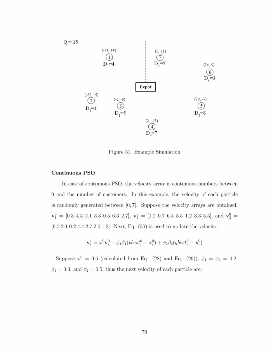
Figure 31. Example Simulation

Continuous PSO

In case of continuous PSO, the velocity array is continuous numbers between

0 and the number of customers. In this example, the velocity of each particle

is randomly generated between [0, 7]. Suppose the velocity arrays are obtained;

v01 = [0.3 4.5 2.1 3.3 0.5 6.3 2.7], v0

2 = [1.2 0.7 6.4 3.5 1.2 3.3 5.5], and v03 =

[6.5 2.1 0.2 4.4 2.7 2.0 1.2]. Next, Eq. (30) is used to update the velocity.

v1i = ω0v0

i + φ1β1(pbest0i − x0

i ) + φ2β2(gbest0i − x0

i )

Suppose ω0 = 0.6 (calculated from Eq. (28) and Eq. (29)), φ1 = φ2 = 0.2,

β1 = 0.3, and β2 = 0.5, thus the next velocity of each particle are:

79

Figure 32. Particle 1: initial solution


80


Particle 1

v11 = 0.6×

0.34.52.13.30.56.32.7

+0.2×0.3×

1− 12− 23− 34− 45− 56− 67− 7

+0.2×0.5×

6− 17− 21− 32− 43− 54− 65− 7

=

0.683.201.061.780.103.581.42

Accordingly, v1

1 = [0.68 3.20 1.06 1.78 0.10 3.58 1.42]

Particle 2

v12 = 0.6×

1.20.76.43.51.23.35.5

+0.2×0.3×

7− 71− 12− 23− 34− 45− 56− 6

+0.2×0.5×

6− 77− 11− 22− 33− 44− 55− 6

=

0.621.023.742.000.621.883.20

Again, v1

2 = [0.62 1.02 3.74 2.00 0.62 1.88 3.20]

81

Particle 3

v13 = 0.6×

6.52.10.24.42.72.01.2

+0.2×0.3×

6− 67− 71− 12− 23− 34− 45− 5

+0.2×0.5×

6− 67− 71− 12− 23− 34− 45− 5

=

3.901.260.122.641.621.200.72

Finally, v1

3 = [3.90 1.26 0.12 2.64 1.62 1.20 0.72]

Next, Eq. (31) is used to update the velocity. Note that if x1ij > xmax then

x1ij = xmax and if x1ij < xmin then x1ij = xmin where xmax = 7, xmin = 0 for this

example.

x1i = x0

i + v1i

Particle 1

max

7.00,

1 + 0.682 + 3.203 + 1.064 + 1.785 + 0.106 + 3.587 + 1.42

=

1.685.264.065.785.107.007.00

= x1

1

x11 = [1.68 5.26 4.06 5.78 5.10 7.00 7.00]

Particle 2

max

7.00,

7 + 0.621 + 1.022 + 3.743 + 2.004 + 0.625 + 1.886 + 3.20

=

7.002.025.745.004.626.887.00

= x1

2

x12 = [7.00 2.02 5.74 5.00 4.62 6.88 7.00]

82

Particle 3

max

7.00,

6 + 3.907 + 1.261 + 0.122 + 2.643 + 1.624 + 1.205 + 0.72

=

7.007.001.124.643.625.207.00

= x1

3

x13 = [7.00 7.00 1.12 4.64 3.62 5.20 7.00]

Next, the solution arrays are decoded in order to obtain the route configura-

tions and the total distance of each particle. In this example, the position array

of particle 1 is x11 = [1.68 5.26 4.06 5.78 5.10 7.00 7.00]. The numbers in

the elements are the rank of each customer. The numbers are sorted increasingly.

Thus, customer 1 is the first and customer 3 is the second. In case of ties numbers,

customer 6 and 7 for this particle, the velocity will be use as the rank numbers.

For example, v016 = 3.58 and v017 = 1.42 (the velocity element 6 = 3.58 and ele-

ment 7 = 1.42). In this case, customer 7 is served before customer 6. The route

configuration of particle 1 is 1-3-2-5-4-7-6 which the vehicle capacity limit divides

it into 3 trips as shown in Fig. 35. The fitness value is 191.

Particle 2 is x12 = [7.00 2.02 5.74 5.00 4.62 6.88 7.00] which

can be routed as 2-5-4-3-6-1-7. Likewise, the vehicle capacity limit divides it

into 3 trips as shown in Fig. 36. The fitness value is 211. Particle 3 is

x13 = [7.00 7.00 1.12 4.64 3.62 5.20 7.00] which can be routed as 3-5-4-

6-7-2-1. The vehicle capacity limit divides it into 3 trips as shown in Fig. 37.

The fitness value is 195. The next iteration starts after the pbest and gbest are

updated. pbest11 = pbest01 because f(x11) 66 f(pbest01). Likewise, pbest12 = pbest02

and pbest13 = pbest03 because the fitness values of these particles are not improving.

gbest is still the same, gbest1 = gbest0 = x03. This procedure executes iteratively

until the maximum iteration count, T , is reached. Table 12 shows the mechanism

of the updating of pbest and gbest.

83

Figure 35. Particle 1: solution of the 1st iteration (continuous)


84


Table 11. pbest and gbest updating (continuous PSO)

Iteration (t) f(xt1) f(pbestt1) f(xt

2) f(pbestt2) f(xt3) f(pbestt3) f(gbestt)

0 178 178 182 182 165 165 1651 191 178 211 182 195 165 1652 150 150 179 179 190 165 1503 165 150 160 160 195 165 150...

......

......

......

...

85

Discrete PSO

Fig. 32, Fig. 33, and Fig. 34 are again used as three initial solutions, as the

last. However, the encoded arrays are now different—the numbers in the elements

are between 0 and n − 1 where n is the number of customers. Thus, the initial

arrays are x01 = [0 1 2 3 4 5 6], x0

2 = [6 0 1 2 3 4 5], and x03 = [5 6 0 1 2 3 4].

Next, pbest0i is memorized and gbest0 = arg mini∈{1,2,..,7} f(x0i ). In this particular

example, gbest0 = x03 which yields the fitness value = 165.

In case of continuous PSO, the velocity array is continuous numbers between 0

and the number of customers. However, in case of the discrete PSO, the velocity of

each particle is a continuous number which is randomly generated between [−4, 4]

because of the discussion in Section 3.2. Suppose the velocity arrays are obtained;

v01 = [−1.2 2.5 0.5 − 3.3 − 0.5 1.1 − 2.7], v0

2 = [1. 2 − 3.7 0.3 3.5 − 1.2 −

1.1 − 2.0], and v03 = [1.5 2.1 − 3.5 − 2.0 2.7 2.0 − 3.7]. Next, Eq. (30) and

Eq. (50) are used to update the velocity.

v1i = ω0v0

i + φ1β1(pbest0i − x0

i ) + φ2β2(gbest0i − x0

i )

v1i = sig(v1

i ) =7

1 + e−v1i

Suppose ω0 = 0.5 (calculated from Eq. (28) and Eq. (29)), φ1 = φ2 = 0.2,

β1 = 0.7, and β2 = 0.2, thus the next velocity of each particle are:

Particle 1

v11 = 0.5×

−1.22.50.5−3.3−0.5

1.1−2.7

+0.2×0.7×

0− 01− 12− 23− 34− 45− 56− 6

+0.2×0.2×

5− 06− 10− 21− 32− 43− 54− 6

=

−0.401.450.17−1.73−0.33

0.47−1.43

86

v11 =

71+e0.40

71+e−1.45

71+e−0.17

71+e1.73

71+e0.33

71+e−0.47

71+e1.43

=

2.805.663.791.052.924.301.35

v11 = [2.80 5.66 3.79 1.05 2.92 4.30 1.35]

Particle 2

v12 = 0.5×

1.2−3.7

0.33.5−1.2−1.1−2.0

+0.2×0.7×

6− 60− 01− 12− 23− 34− 45− 5

+0.2×0.2×

5− 66− 00− 11− 22− 33− 44− 5

=

0.56−1.61

0.111.71−0.64−0.59−1.04

v12 =

71+e−0.56

71+e1.61

71+e−0.11

71+e−1.71

71+e0.64

71+e0.59

71+e1.04

=

4.451.163.695.922.412.491.82

Accordingly, v1

2 = 4.45 1.16 3.69 5.92 2.41 2.49 1.82]

Particle 3

v13 = 0.5×

1.52.1−3.5−2.0

2.72.0−3.7

+0.2×0.7×

5− 56− 60− 01− 12− 23− 34− 4

+0.2×0.2×

5− 56− 60− 01− 12− 23− 34− 4

=

0.751.05−1.75−1.00

1.351.00−1.85

87

v13 =

71+e−0.75

71+e−1.05

71+e1.75

71+e1.00

71+e−1.35

71+e−1.00

71+e1.85

=

4.755.181.031.885.555.110.95

Accordingly, v1

3 = [4.75 5.18 1.03 1.88 5.55 5.11 0.95]

Then, Eq. (51) and Eq. (52) are used to find the position of each particle.

Suppose σ = 0.7, and β are generated separately.

x1 = round(vti + (7− 1)× σ × β)

x1ij =

{Z − 1 : if x1ij > Z − 10 : if x1ij < 0

Particle 1

x11 = max

6, round

2.805.663.791.052.924.301.35

+ 6× 0.7×

0.120.550.330.050.730.390.62

=

3651664

= x1

1

x11 = [3 6 5 1 6 6 4]

Particle 2

x12 = max

6, round

4.451.163.695.922.412.491.82

+ 6× 0.7×

0.050.170.040.920.150.330.07

=

5246342

= x1

2

x12 = [5 2 4 6 3 4 2]

88

Table 12. pbest and gbest updating (discrete PSO)

Iteration (t) f(xt1) f(pbestt1) f(xt

2) f(pbestt2) f(xt3) f(pbestt3) f(gbestt)

0 178 178 182 182 165 165 1651 211 178 205 182 177 165 1652 200 178 190 182 200 165 1653 170 170 150 150 180 165 150...

......

......

......

...

Particle 3

x13 = max

6, round

4.755.181.031.885.555.110.95

+ 6× 0.7×

0.770.000.560.020.630.880.21

=

6532662

= x1

3

x13 = [6 5 3 2 6 6 2]

The decoding method of the discrete PSO is same as the continuous version.

Particle 1 position array is x11 = [3 6 5 1 6 6 4]. The numbers in the elements

are the rank of each customer. The numbers are sorted increasingly. vti is used

when there is a tie. Thus, particle 1 can be routed as 4-1-7-3-5-6-2. Particle 2’s

position array is x12 = [5 2 4 6 3 4 2] which can be routed as 2-7-5-6-3-1-4.

Particle 3’s position array is x13 = [6 5 3 2 6 6 2] which can be routed as

7-4-3-2-1-6-5. The route configurations of the particle 1, 2, and 3 are shown in Fig.

38, Fig. 39, and Fig. 40, respectively.

As in the continuous version, the next iteration starts after pbest and gbest

are updated. pbest11 = pbest01 because f(x11) > pbest01. Similarly, pbest12 = pbest02

and pbest13 = pbest03 because no improve on fitness values. This procedure executes

iteratively until the maximum iteration count, T , is reached.

89

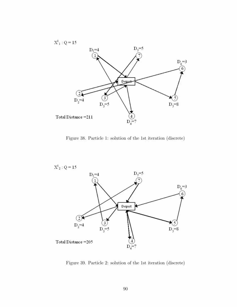
Figure 38. Particle 1: solution of the 1st iteration (discrete)


90


3.6 Computational Experiments

In order to demonstrate the effectiveness and performance of the proposed

methods, computational experiments on two benchmark data sets have been con-

ducted. The first set is Christofides benchmark data set [78]. This data set has 14

benchmark problems in which the number of customers varies between 50 and 199.

The second set is Chen’s benchmark data set [71]. The 15 benchmark problems

from Chen’s benchmark data set were selected in a manner similar to that in the

studies of Ai and Kachitvichyanukul [73] and Kim and Son[74].

3.6.1 Competitive approaches

Two PSO-based approaches were selected for comparison with the proposed

approaches. The first approach was the SR-2, which was proposed by Ai and Ka-

chitvichyanukul [73]. The second approach was the Prob MAT which was proposed

by Kim and Son [74].

91

In order to produce comparable results among competitive approaches, the

local improvement step of SR-2 and Prob MAT was changed to the similar methods

which I used in the proposed approaches. That is to say, the 2-Opt exchange,

Or-Opt exchange, 1-1 exchange, and 1-0 exchange methods were consecutively

deployed to all competitive approaches. The first improvement strategy (FI) [33]

has been used to guide the choice of the next move to be performed (as shown in

Fig. 30).


The PSO parameters of my proposed methods were set as follows: the number

of particles, N = 40; the number of sub-swarms, S = 4; the maximum number

of iterations, T = 1000; the maximum inertia weight, ωmax = 0.7; the minimum

inertia weight, ωmin = 0.3; the step size of the inertia weight, ∆ω = 0.1; the

cognitive and social factors, φ1 = φ2 = 0.2; the bounce factor, δ = 0.5; the

standard deviation (for the discrete PSO version), σ = 0.1n where n is the number

of customers.

3.6.3 Results and discussions

The algorithms have been implemented in C++ language using Microsoft

Visual Studio 2010 on a Windows 7 Intel Xeon, 2.4 GHz processor with 64 GB

of RAM. Since the algorithms in this study were stochastic search algorithms,

the approaches were repeated 15 times for each benchmark problem, and the best

fitness values and the worst fitness values of each algorithm have been reported.

Table 13 shows the best and the worst results among 15 trials of all competi-

tive algorithms on the problem set of Christofides et al. [78]. The best performance

among competitive algorithms are highlighted in boldface. The BKS stands for

the best known solution. As the results show, the discrete PSO outperforms other

92

competitive algorithms by providing 10 best solutions on the 14 benchmark prob-

lems. The Prob MAT, SR-2, and continuous PSO yield 7, 6, and 5 best solutions

on the 14 benchmark problems, respectively.

93

Table 13. Computational results of Christofides’ benchmark data sets

Problem Num. Num.Fitness value (distance)

Cust. Route BKS SR-2 Prob MAT Continuous PSO Discrete PSO

Best Worst Best Worst Best Worst Best Worst

vrpnc1 50 5 524.61 524.61 679.32 524.61 727.45 524.61 665.13 531.16 682.32vrpnc2 75 10 835.26 842.73 865.32 835.26 987.16 835.26 894.84 835.26 867.90vrpnc3 100 8 826.14 829.40 894.56 832.46 965.35 843.80 902.65 826.14 892.65vrpnc4 150 12 1028.42 1048.89 1128.25 1047.72 1168.23 1106.05 1204.67 1046.32 1165.43vrpnc5 199 17 1291.45 1323.89 1406.39 1332.06 1506.22 1428.12 1487.05 1325.68 1408.66vrpnc6 50 6 555.43 555.43 580.24 555.43 612.65 555.43 562.34 555.43 605.41vrpnc7 75 11 909.68 918.65 943.21 913.24 968.26 913.24 942.28 913.24 948.65vrpnc8 100 9 865.94 882.83 894.17 865.94 908.16 889.04 912.45 865.94 901.06vrpnc9 150 14 1162.55 1185.41 1214.69 1176.20 1248.67 1432.56 1632.90 1173.25 1212.63vrpnc10 199 18 1395.85 1428.46 1479.93 1443.25 1572.18 1502.23 1574.49 1431.16 1482.29vrpnc11 120 7 1042.11 1048.56 1089.72 1062.39 1189.43 1172.06 1289.33 1046.35 1272.35vrpnc12 100 10 819.56 819.56 826.37 819.56 845.32 819.56 832.15 819.56 839.42vrpnc13 120 11 1541.14 1546.20 1592.17 1548.06 1619.22 1569.25 1582.48 1544.83 1578.49vrpnc14 100 11 866.37 866.37 877.29 866.37 889.08 869.43 879.53 866.37 881.29

94

Figure 41. The comparison on the small-size problems of Christofides’ data set

However, if I divide the benchmark problems into two classes: the small-size

benchmark problems (n 6 75) and the large-size benchmark problems (n > 75)

where n is the number of customers, there are 4 small-size benchmark problems and

10 large-size benchmark problems in this data set. The continuous PSO and the

Prob MAT yielded 4 best solutions on the 4 small size benchmark problems while

the discrete PSO and the SR-2 yielded 3 and 2 best solutions on the 4 small-size

benchmark problems, respectively (Fig. 41).

For the large-size benchmark problems (n > 75), the discrete PSO provides 8

best solutions on the 10 large-size benchmark problems. The SR-2, Prob MAT and

continuous PSO render 4, 3, and 1 best solutions on the 10 large-size benchmark

problems, respectively (Fig. 42).

95

Figure 42. The comparison on the large-size problems of Christofides’ data set

Table 14 shows the best and the worst results among 15 trials of all competitive

algorithms on the problem set of Chen et al. [71]. The discrete PSO provides

10 best solutions on the 15 benchmark problems. The SR-2, Prob MAT, and

continuous PSO generate 8, 8, and 6 best solutions on the 15 benchmark problems,

respectively. In general, the discrete PSO dominates other competitive algorithms

while the continuous PSO is less effective on Chen’s problem set.

There are 11 small-size benchmark problems and 4 large-size benchmark prob-

lems in Chen’s data set. Prob MAT provides 7 best solutions on the 11 small-size

benchmark problems. The SR-2, continuous PSO, and discrete PSO respectively

yielded 6, 6, and 5 best solutions on the 11 large-size benchmark problems (Fig.

43).

96

Table 14. Computational results of Chen’s benchmark data sets

Problem Num. Num.Fitness value (distance)

Cust. Route BKS SR-2 Prob MAT Continuous PSO Discrete PSO

Best Worst Best Worst Best Worst Best Worst

an33k5 32 5 661 661 693 661 712 661 697 664 704an46k7 45 7 914 915 967 914 982 914 953 915 980an60k9 59 9 1354 1355 1367 1355 1382 1354 1376 1358 1379bn35k5 34 5 955 955 967 955 974 955 968 955 975bn45k5 44 5 751 751 782 754 793 751 776 753 784bn68k9 67 9 1272 1277 1289 1275 1293 1281 1293 1276 1287en30k3 29 3 534 534 547 534 557 534 545 536 550en51k5 50 5 521 524 543 524 547 527 538 523 537en76k7 75 7 682 682 695 687 702 685 693 682 689fn72k4 71 4 237 237 246 237 256 239 249 237 250fn135k7 134 7 1162 1162 1183 1170 1203 1205 1217 1162 1178mn101k10 100 10 820 822 831 821 835 839 845 820 833mn121k7 120 7 1034 1039 1045 1036 1049 1087 1106 1035 1075pn76k4 75 4 593 596 602 594 611 603 614 594 601pn101k4 100 4 681 684 699 684 701 686 694 684 698

97

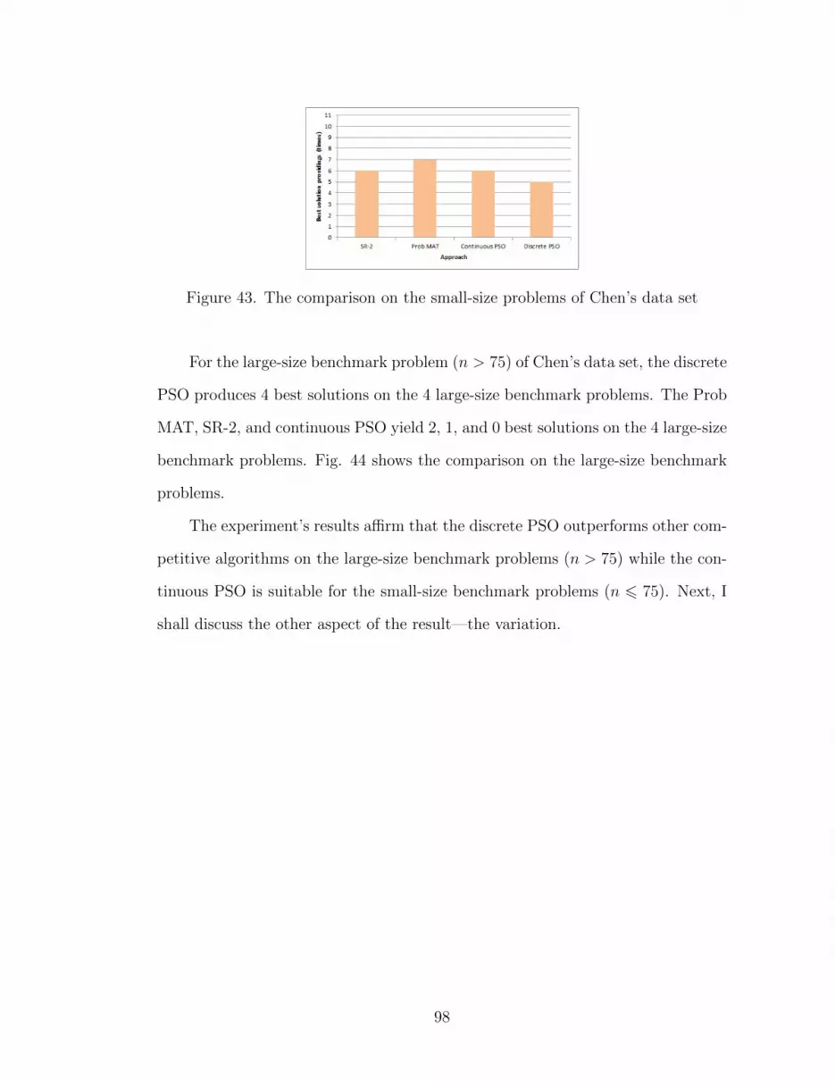
Figure 43. The comparison on the small-size problems of Chen’s data set

For the large-size benchmark problem (n > 75) of Chen’s data set, the discrete

PSO produces 4 best solutions on the 4 large-size benchmark problems. The Prob

MAT, SR-2, and continuous PSO yield 2, 1, and 0 best solutions on the 4 large-size

benchmark problems. Fig. 44 shows the comparison on the large-size benchmark

problems.

The experiment’s results affirm that the discrete PSO outperforms other com-

petitive algorithms on the large-size benchmark problems (n > 75) while the con-

tinuous PSO is suitable for the small-size benchmark problems (n 6 75). Next, I

shall discuss the other aspect of the result—the variation.

98

Figure 44. The comparison on the large-size problems of Chen’s data set

Relative percent deviation

The relative percent deviation (RDP) measures the deviation of the algo-

rithm’s output compared to the best known fitness value. The calculation of the

RDP is shown in Eq.(58):

RPD =

(G− C∗

C∗× 100

)(58)

where G is the global best of the approach and C∗ is the best known value. The

average RDP (RDP ) is calculated with Eq.(59):

RPD =

∑Ni=1RPDi

N(59)

where N is the number of benchmark problems in the data set.

99

Table 15. Relative Percent Deviation (RPD) of Christofides’ benchmark data sets

Problem Num. Num. SR-2 Prob. MAT Continuous PSO Discrete PSO

Cust. Route Best Worst Best Worst Best Worst Best Worst

vrpnc1 50 5 0.00 29.49 0.00 38.66 0.00 26.79 1.25 30.06vrpnc2 75 10 0.89 3.60 0.00 18.19 0.00 7.13 0.00 3.91vrpnc3 100 8 0.39 8.28 0.77 16.85 10.58 15.15 2.65 9.08vrpnc4 150 12 1.99 9.71 1.88 13.59 7.55 17.14 1.74 13.32vrpnc5 199 17 2.51 16.61 3.14 16.63 10.58 15.15 2.65 9.08vrpnc6 50 6 0.00 4.47 0.00 10.30 0.00 1.24 0.00 9.00vrpnc7 75 11 0.99 3.69 0.39 6.44 0.39 1.60 0.39 4.28vrpnc8 100 9 1.95 3.26 0.00 4.88 2.67 5.37 0.00 4.06vrpnc9 150 14 1.97 4.48 1.17 7.41 23.23 40.46 0.92 4.31vrpnc10 199 18 2.34 6.02 3.40 12.63 7.62 12.80 2.53 6.19vrpnc11 120 7 0.62 4.57 1.95 14.14 12.47 23.72 0.41 22.09vrpnc12 100 10 0.00 0.83 0.00 3.14 0.00 1.54 0.00 2.42vrpnc13 120 11 0.33 3.31 0.45 5.07 1.82 2.68 0.24 2.42vrpnc14 100 11 0.00 1.26 0.00 2.62 0.35 1.52 0.00 1.72

Average RPD: RPD 1.00 7.12 0.94 12.18 4.92 11.89 0.72 8.64Interval: (Worst RPD − Best RPD) 6.12 11.24 6.97 7.91

100

Table 16. Relative Percent Deviation (RPD) of Chen’s benchmark data sets

Problem Num. Num. SR-2 Prob. MAT Continuous PSO Discrete PSO

Cust. Route Best Worst Best Worst Best Worst Best Worst

an33k5 32 5 0.00 4.84 0.00 7.72 0.00 5.45 0.45 6.51an46k7 45 7 0.11 5.80 0.00 7.44 0.00 4.27 0.11 7.22an60k9 59 9 0.07 0.96 0.07 2.07 0.00 1.62 0.30 1.85bn35k5 34 5 0.00 1.26 0.00 1.99 0.00 1.36 0.00 2.09bn45k5 44 5 0.00 4.13 0.40 5.59 0.00 3.33 0.27 4.39bn68k9 67 9 0.39 1.34 0.24 1.65 0.71 1.65 0.31 1.18en30k3 29 3 0.00 2.43 0.00 4.31 0.00 2.06 0.37 3.00en51k5 50 5 0.58 4.22 0.58 4.99 1.15 3.26 0.38 3.07en76k7 75 7 0.00 1.91 0.73 2.93 0.44 1.61 0.00 1.03fn72k4 71 4 0.00 3.80 0.00 8.02 0.84 5.06 0.00 5.49fn135k7 134 7 0.00 1.81 0.69 3.53 3.70 4.73 0.00 1.38mn101k10 100 10 0.24 1.06 0.12 1.83 2.32 3.05 0.00 1.59mn121k7 120 7 0.48 1.06 0.19 1.45 5.13 6.96 0.10 3.97pn76k4 75 4 0.51 1.52 0.17 3.04 1.69 3.54 0.17 1.35pn101k4 100 4 0.44 2.64 0.44 2.94 0.73 1.91 0.44 2.50

Average RPD: RPD 0.20 2.44 0.26 3.70 1.19 3.17 0.17 2.86Interval: (Worst RPD − Best RPD) 2.24 3.44 1.98 2.69

101

Table 15 and Table 16 show the RDP of the results from Table 13 and Table 14,

respectively. From Table 15, the discrete PSO provides the smallest average RPD

(0.72) on the best solution results. Interestingly, even the discrete PSO provides

the best average RPD; however, the interval value between the best RDP and

the worst RDP is worse than in the SR-2 and the continuous PSO. This means

that the discrete PSO generates more fluctuating outputs than the SR-2 and the

continuous PSO. Similarly, as in Table 16, the discrete PSO yields the smallest

average RPD (0.16) on the best solution results. Nonetheless, the interval values

between RDP and the worst RDP is worse than the SR-2 and the continuous

PSO.

This phenomena can be explained by the “noisy-fitness evaluation”. Since the

discrete decoding method uses the sigmoid function as Eq.(50) and the discrete

number generation function as Eq.(51), the different element fitness value can be

obtained from the identical particle (the so-called noisy-fitness evaluation). Thus,

the discrete PSO generates solutions with varying success.

The Prob MAT provides the highest value of the interval between the worst

RPD and the best RPD. This can be explained by the nature of the algorithm

itself. The Prob MAT randomly assigns the probability to each array in the matrix,

in the extreme. There is nothing controlling the noise. In contrast, the continuous

PSO and SR-2 are noiseless fitness evaluation methods.

In fact, the noisy-fitness evaluation enhances the performance of the search

algorithms. The wide interval value between the best fitness value and the worst

fitness value is compensated for by the chance to obtain the better fitness value.

On the other hand, the higher noisy-fitness evaluation degrades the convergence

rate of the PSO method, as in the Prob MAT.

102

3.7 Conclusions

This chapter proposed a continuous PSO and a discrete PSO extensions for

novel adaptive PSO: the Survival Sub-swarms Adaptive Particle Swarm Optimiza-

tion with velocity-line bouncing (SSS-APSO-vb), presented in Chapter 2. The

computational results on the benchmark data sets showed that the proposed PSO-

based algorithms are comparable with recent competitive algorithms. The contin-

uous PSO works well on the small-size problems (n 6 75), while the discrete PSO

outperforms other algorithms on the large-size problems (n > 75).

The performance of the proposed methods are enhanced by the following rea-

sons. First, the performance of the novel PSO improves the exploration and ex-

ploitation abilities. Second, in the case of the discrete PSO, the noisy-fitness

evaluation, which can be controlled by the predefined parameter (σ), elevates the

search performance of the approach through the search space. Third, the quality

of the solutions is improved by the low-cost local improvement methods.

Although the parameter settings on the proposed algorithms were obtained

from a preliminary study, they may not be suitable for problems from different

domains. Consequently, a practitioner needs a preliminary study to design a robust

parameter settings.

103

List of References

[1] G. Dantzig and J. Ramser, “The truck dispatching problem,” ManagementScience, vol. 6, pp. 80–91, 1959.

[2] P. Toth and D. Vigo, The Vehicle Routing Problem, 1st. edn. Philadelphia,PA, USA: Society for Industrial and Applied Mathematics, 2002.

[3] A. V. Breedam, “Improvement heuristics for the vehicle routing problem basedon simulated annealing,” European Journal of Operational Research, vol. 86,pp. 480–490, 1995.

[4] W.-C. Chiang and R. A. Russell, “Simulated annealing metaheuristics for thevehicle routing problem with time windows,” Annals of Operations Research,vol. 63, pp. 3–27, 1996.

[5] C. Ren and S. Li, “New genetic algorithm for capacitated vehicle routingproblem,” Advances in Computer Science and Information Engineering, vol. 1,pp. 695–700, 2012.

[6] M. Gendreau, A. Hertz, and G. Laporte, “A tabu search heuristic for thevehicle routing problem,” Management Science, vol. 4(10), pp. 1276–1290,1994.

[7] B. Bullnheimer, R. F. Hartl, and C. Strauss, “An improved ant system algo-rithm for vehicle routing problem,” Annals of Operations Research, vol. 89,pp. 319–328, 1999.

[8] A. Torki, S. Somhon, and T. Enkawa, “A competitive neural network algo-rithm for solving vehicle routing problem,” Computers & Industrial Engineer-ing, vol. 33, pp. 473–476, 1997.

[9] J. Zhang, W.-N. Chen, Z.-H. Zhan, W.-J. Yu, Y.-L. Li, N. Chen, and Q. Zhou,“A survey on algorithm adaptation in evolutionary computation,” Frontiersof Electrical and Electronic Engineering, vol. 7(1), pp. 16–31, 2012.

[10] R. Kuo, F. E. Zulvia, and K. Suryadi, “Hybrid particle swarm optimizationwith genetic algorithm for solving capacitated vehicle routing problem withfuzzy demand - a case study on garbage collection system,” Applied Mathe-matics and Computation, vol. 219, pp. 2574–2588, 2012.

[11] G. Laporte, “The vehicle routing problem: an overview of exact and approx-imate algorithms,” European Journal of Operational Research, vol. 59, pp.345–359, 1992.

[12] G. Laporte, H. Mercure, and Y. Nobert, “An exact algorithm for the asym-metrical capacitated vehicle routing,” Networks, vol. 16(1), pp. 33–46, 1986.

104

[13] N. Christofides, A. Mingozzi, and P. Toth, “Exact algorithms for the vehi-cle routing problem, based on spanning tree and shortest path relaxations,”Mathematical Programming, vol. 20, pp. 255–282, 1981.

[14] T. K. Ralphs, “Parallel branch and cut for vehicle routing,” Ph.D. dissertation,Cornell University, 1995.

[15] M. L. Balinski and R. E. Quandt, “On an integer program for a deliveryproblem,” Operations Research, vol. 12(2), pp. 300–304, 1964.

[16] M. R. Rao and S. Zionts, “Allocation of transportation units to alternativetrips - a column generation scheme with out-of-killer subproblems,” Opera-tions Research, vol. 16(1), pp. 52–63, 1968.

[17] J. Desrosiers and F. Soumis, “Routing with time windows by column genera-tion,” Networks, vol. 14(4), pp. 545–565, 1984.

[18] Y. Agarwal, K. Mathur, and H. M. Salkin, “A set-partitioning-based exactalgorithm for the vehicle routing problem,” Networks, vol. 19(7), pp. 731–749,1989.

[19] G. Desaulniers, J. Desrosiers, and M. M. Solomon, Column Generation. NewYork, USA: Springer, 2010.

[20] M. Drexl, “Rich vehicle routing in theory and practice,” Logistics Research,vol. 5, pp. 47–63, 2012.

[21] S. Ropke, “Heuristic and exact algorithm for vehicle routing problem,” Ph.D.dissertation, University of Copenhagen, 2005.

[22] R. Baldacci, A. Mingozzi, and R. Roberti, “Recent exact algorithms for solvingthe vehicle routing problem under capacity and time window constraints,”European Journal of Operational Research, vol. 218, pp. 1–6, 2012.

[23] G. Clarke and J. Wright, “Scheduling of vehicles from a central depot toa number of delivery points,” Operations Research, vol. 12(4), pp. 568–581,1964.

[24] G. Laporte, M. Gendreau, J.-Y. Potvin, and F. Semet, “Classical and mod-ern heuristics for the vehicle routing problem,” International Transactions inOperational Research, vol. 7, pp. 285–300, 2000.

[25] S. Lin, “Computer solutions of the traveling salesman problem,” Bell SystemTechnical Jouranl, vol. 44, pp. 2245–2269, 1965.

[26] A. Van Breedam, “An analysis of the behavior of heuristics for the vehiclerouting problem for a selection of problems with vehicle-related, customer-related, and time-related constraints.”

105

[27] B. E. Gillett and L. R. Miller, “A heuristic algorithm for the vehicle dispatchproblem,” Operations Research, vol. 22, pp. 340–349, 1974.

[28] M. L. Fisher, “The lagrangian relaxation method for solving integer program-ming problem,” Management Science, vol. 27(1), pp. 1–18, 1981.

[29] J. Bramel and D. Simchi-Levi, “A location based heuristic for general routingproblems,” Operations Research, vol. 43(4), pp. 649–660, 1995.

[30] I. H. Osman, “Metastrategy simulated annealing and tabu search algorithmsfor the vehicle routing problem,” Annals of Operations Research, vol. 41, pp.421–451, 1993.

[31] S. Lin and B. W. Kernighan, “An effective heuristic algorithm for the travelingsalesman problem,” Operations Research, vol. 21(2), pp. 498–516, 1973.

[32] I. Or, “Traveling salesman-type combinatorial problems and their relationto the logistics of regional blood banking,” Ph.D. dissertation, NorthwesternUniversity, 1976.

[33] A. V. Breedam, “Comparing descent heuristics and metaheuristics for thevehicle routing problem,” Computers & Operations Research, vol. 28, pp. 289–315, 2001.

[34] O. Braysy and M. Gendreau, “Vehicle routing problem wiht time windows,part i: route construction and local search algorithms,” Transportation Sci-ence, vol. 39(1), pp. 104–118, 2005.

[35] B. Funke, T. Grunert, and S. Irnich, “Local search for vehicle routing andscheduling problems: review and conceptual integration,” Heuristics, vol. 11,pp. 267–306, 2005.

[36] R. K. Ahuja, O. Ergun, J. B. Orlin, and A. P. Punnen, “A survey of verylarge-scale neighborhood search techniques,” Discrete Applied Mathematics,vol. 123, pp. 75–102, 2002.

[37] M. Gendreau and J.-Y. Potvin, “Metaheuristics in combinatorial optimiza-tion,” Annals of Operations Research, vol. 140, pp. 189–213, 2005.

[38] V. Cerny, “Thermodynamical approach to the traveling salesman problem,”Optimization Theory and Applications, vol. 45(1), pp. 41–51, 1985.

[39] S. Kirkpatrick, C. D. Galatt, and M. P. Vecchi, “Optimization by simulatedannealing,” Science, vol. 220, pp. 671–680, 1983.

[40] M. Gendreau, G. Laporte, and J.-Y. Potvin, The vehicle routing problem.Philadelphia, USA: SIAM, 2002, ch. Mataheuristics for the capacitated VRP,pp. 129–154.

106

[41] J.-F. Cordeau, M. Gendreau, G. Laporte, J.-Y. Potvin, and F. Semet, “Aguide to vehicle routing heuristics,” Operational Research Society, vol. 53(5),pp. 512–522, 2002.

[42] F. Glover, “Future paths for integer programming and links to artificial intel-ligence,” computers & Operations Research, vol. 13(5), pp. 533–549, 1986.

[43] E. Taillard, “Parallel iterative search methods for vehicle routing problems,”Networks, vol. 23(8), pp. 661–673, 1993.

[44] P. Toth and D. Vigo, “The granular tabu search (and its application to thevehicle routing problem),” Bologna, Italy, Tech. Rep. OR/98/9, 1998.

[45] Y. Rochat and E. D. Taillard, “Probabilistic diversificaiton and intensificationin local search for vehicle routing,” Heuristics, vol. 1(1), pp. 147–167, 1995.

[46] J.-F. Cordeau, G. Laporte, and A. Mercier, “A unified tabu search heuristic forvehicle routing problems with time windows,” Operational Research Society,vol. 52(8), pp. 928–936, 2001.

[47] J. H. Holland, Adaptation in Natural and Artificial Systems. Michigan, USA:The University of Michigan Press, 1975.

[48] M. Gen and R. Chen, Genetic Algorithms & Engineering Optimization. NewYork, USA: John Wiley & Sons, 2000.

[49] B. M. Baker and M. Ayechew, “A genetic algorithm for the vehicle routingproblem,” Computers & Operations Research, vol. 30(5), pp. 787–800, 2003.

[50] A. Colorni, M. Dorigo, and V. Maniezzo, “Distributed optimization by antcolonies,” in Proceedings of the Europeon Conference on Artificial Life, 1991,pp. 134–142.

[51] M. Dorigo and T. Stutzle, Handbook of Metaheuristics. Boston, USA:Springer, 2003, ch. The Ant Colony Optimization: Algorithms, Applications,and Advances, pp. 251–285.

[52] H. Kawamura, M. Yamamoto, T. Mitamura, M. K. Suzuki, and A. Ohuchi,“Cooperative search on pheromone communication for vehicle routing prob-lems,” IEICE Transactions on Fundamentals of Electronics, Communicationsand Computer Sciences, vol. E81-A(6), pp. 1089–1096, 1998.

[53] B. Bullnheimer, R. F. Hartl, and C. Strauss, Meta-Heuristics. Boston, USA:Springer, 1999, ch. Applying the ANT System to the Vehicle Routing Problem,pp. 285–296.

[54] J. Kennedy and R. Eberhart, “A discrete binary version of the particle swarmalgorithm,” in Proceedings of IEEE International Conference on Systems,Man, and Cybernetics, 1997, pp. 4104–4108.

107

[55] J. Kennedy and R. C. Eberhart, Swarm Intelligence, 1st. edn. San Diago,CA, USA: Academic Press, 2001.

[56] L. Osadciw and K. Veeramachaneni, Particle Swarm Optimization. Vienna,Austria: In-Tech, 2009, ch. Particle Swarms for Continuous, Binary, and Dis-crete Search Spaces, pp. 451–460.

[57] M.-S. Tsai and W.-C. Wu, Particle Swarm Optimization. Vienna, Austria:In-Tech, 2009, ch. A Novel Binary Coding Particle Swarm Optimization forFeeder Reconfiguration, pp. 437–450.

[58] B. Al-kazemi and C. K. Mohan, “Multi-phase discrete particle swarm opti-mization,” in Proceedings of the Fourth Internation Workshop on Fromtiersin Evolutionary Algorithms, 2000.

[59] B. Al-kazemi, “Multi-phase generalization the particle swarm optimization al-gorithm,” in Proceedings of the 2002 Congress on Evolutionary Computation,2002.

[60] S. Yang, M. Wang, and L. Jiao, “A quantum particle swarm optimization,”in Proceedings of the IEEE Congress on Evolutionary Computation, 2004, pp.320–324.

[61] M. A. Khanesar, H. Tavakoli, M. Teshnehlab, and M. A. Shoorehdeli, ParticleSwarm Optimization. Vienna, Austria: In-Tech, 2009, ch. Novel BinaryParticle Swarm Optimization, pp. 1–10.

[62] M. Clerc, New Optimization Techniques in Engineering. New York, USA:Springer Berlin Heidelberg, 2004, ch. Discrete Particle Swarm Optimization:Illustrated by the Traveling Salesman Problem, pp. 219–239.

[63] W. liang Zhong, J. Zhang, and W. neng Chen, “A novel discrete particleswarm optimization to solve traveling salesman problem,” in Proceedings ofthe IEEE Congress on Evolutionary Computation, 2007, pp. 3283–3287.

[64] W. Pang, K. ping Wang, C. guang Zhou, and L. jiang Dong, “Fuzzy discreteparticle swarm optimization for solving traveling salesman problem,” in Pro-ceedings of the 4th International Conference on Computer and InformationTechnology, 2004, pp. 796–800.

[65] S. Ponnambalam, N. Jawahar, and S. Chandrasekaran, Particle Swarm Op-timization. Vienna, Austria: In-Tech, 2009, ch. Discrete Particle SwarmOptimization Algorithm for Flowshop Scheduling, pp. 397–422.

[66] J. Pugh and A. Martinoli, “Discrete multi-valued particle swarm optimiza-tion,” in Proceedings of the IEEE Swarm Intelligence Symposium, 2006, pp.103–110.

108

[67] J. Pugh, A. Martinoli, and Y. Zhang, “Particle swarm optimization for un-supervised robotic learning,” in Proceedings of the IEEE Swarm IntelligenceSymposium, 2005, pp. 92–99.

[68] E. K. Antonsson, Y. Zhang, and A. Martinoli, “Evolving engineering designtrade-offs,” in Proceedings of the ASME Fifteenth International Conferenceon Design Theory and Methodology, 2003.

[69] J. M. Fitzpatrick and J. J. Grefenstette, “Genetic algorithm in noisy environ-ment,” Machine Learining, vol. 3, pp. 101–120, 1988.

[70] H.-G. Beyer, “Evolutionary algorithms in noisy environments: theoretical is-sues and guidelines for practice,” Computer Methods in Mechanics and AppliedEngineering, vol. 186, pp. 239–267, 2000.




[74] B.-I. Kim and S.-J. Son, “A probability matrix based particle swarm optimiza-tion for the capacitated vehicle routing problem,” Intelligence Manufacturing,vol. 23, pp. 1119–1126, 2012.

[75] N. Norouzi, R. Tavakkoli-Moghaddam, M. Ghazanfari, M. Alinaghian, andA. Salamatbakhsh, “A new multi-objective competitive open vehicle routingproblem solved by particle swarm optimization,” Networks & Spatial Eco-nomics, vol. 12(4), pp. 609–633, 2012.

[76] Y. Marinakis, G.-R. Iordanidou, and M. Marinaki, “Particle swarm optimiza-tion for the vehicle routing problem with stochastic demands,” Applied SoftComputing, vol. 13, pp. 1693–1704, 2013.

[77] F. Belmecheri, C. Prins, F. Yalaoui, and L. Amodeo, “Particle swarm op-timization algorithm for a vehicle routing problem with heterogeneous fleet,mixed backhauls, and time windows,” Intelligent Manufacturing, vol. 24, pp.775–789, 2013.

[78] N. Christofides, A. Mingozzi, and P. Toth, Combinatorial Optimization. NewJersey, USA: John Wiley & Sons, 1979, ch. The Vehicle Routing Problem, pp.315–338.

109

CHAPTER 4

PSO for the Partitioned Vehicle ofa Multi Commodity Recyclables Collection Problem

4.1 Introduction

Logistics can be divided into forward logistics and reverse logistics. Forward

logistics refers to the distribution of materials/goods from one or more original

points to customers. Reverse logistics refers to the collecting of materials/wastes

from customers back to one or more collecting points [1]. The forward logistics has

been fine-tuned and extensively studied for decades. However, the problem study

of reverse logistics is relatively recent. The white paper of the Council of Logistics

Management (CLM), first published the definition of reverse logistics in the early

1990’s:

“... the term often used to refer to the role of logistics in recycling,waste disposal, and management of hazardous materials; a broader per-spective includes all relating to logistics activities carried out in sourcereduction, recycling, substitution, reuse of materials and disposal.” [2]

In the end of 1990’s , Rogers and Tibben-Lembke defined reverse logistics stressing

the goal and the processes involved:

“... the process of planning, implementing, and controlling the efficient,cost-effective flow of raw materials, in-process inventory, finished goods,and related information from the point of consumption to the point oforigin for the purposed of recapturing value or proper disposal.” [3]

Fleischmann summarized the characteristics of reverse logistic as follows:

“... is the process of planning, implementing, and controlling the effi-cient, effective inbound flow and storage of secondary goods and relatedinformation opposite to the traditional supply chain direction for thepurpose of recovering value or proper disposal.” [4]

110

Figure 45. Forward-reverse logistics: source [5]

In conclusion, reverse logistics refers to the logistics activities, which involves

the physical transportation of used products—no longer required by the users—

back to producers to be used again in a market. Reverse logistics includes both

transportation of used products and recyclable waste. Fleischmann [5] presented

the framework of logistics, Fig. 45, in which depicted both forward logistics and

reverse logistics. Reverse logistics can be divided into two systems. The first system

is known as closed-loop system in which a used product is returned to the same

manufacturer in order to remanufacturing and reused. The second system is known

as open-loop system in which a used product and/or packaging (recyclables) is not

returned to the original manufacturer. Seuring and Muller [6] and Brandenburg

et al. [7] provided comprehensive literature reviews on the closed-loop logistics

system. Fleischmann et al. [5] provided broad review on the open-loop logistics

system and related activities. In this study, I focus on the path between customers

and collectors, known as “collection of recyclables”.

111

The collection of recyclables is defined as a fleet of trucks operating to pick-

up recyclables—such as paper, plastic, glass, and metal cans—either curbside or

at customer sites and then taking the materials to a Material Recovery Facility

(MRF) with an objective of minimizing total operational cost. In general, the

cost of the collection program is responsible by the municipality [8]. The waste

collection costs were estimated to be between 60% and 80% of the solid waste man-

agement budget [9, 10]. In order to lower the collection cost, the municipality may

deploy a community aggregation center in which consumers bring their segregated

recyclables to a local facility where the material is stored for pickup by a recycling

service. Accordingly, the recycling company faces the challenging problem of how

to preserve the segregated materials during the transportation. This brings me to

a specific truck configuration problem, known as “partitioned trucks”.

As the literature review of Mohanty [1] suggests, there are a number of advan-

tages of using partitioned trucks for recycling. The labor and processing costs are

reduced by separating the recyclables at the source. The partitions enhance the

volume of materials that can be collected because of shredding and compacting

equipment. In the case of hazardous materials, the partitioned trucks are more

suitable than the traditional trucks. Finally, for preserving the segregated materi-

als, a partitioned truck cost less than employing a specified truck for each type of

materials.

4.2 A Multi Commoditiy Recyclables Collection Problem4.2.1 The truck partition problem

The truck partition problem (TPP) was first introduced by Reimer et al. [11].

The authors derived this model from the study of Wiese and Zelewski [12], in which

formulated the waste creation as an Economic Order Quantity (EOQ) model. Two

closed-from expressions were proposed: the optimal number of trash pick-ups (n∗)

112

and the optimal amount of waste per pick-up (q∗). The formulas are respectively

shown as:

n∗ =

√αβT 2

2Cpf(60)

q∗ =

√2CpfQ

βT(61)

where α is the waste accumulation rate, β is the waste storage costs rate, T is the

time period [0, T ] between two pick-ups, Cpf is the trash pick-up fee, and Q is the

amount of accumulated materials over a given time period [0, T ]. This formulation

improves our estimation of the amount of materials picked up and the interval time

between two pick-ups.

Reimer el al. [11] proposed the truck size problem model which known as

Recycling Vehicle Sizing Problem (RVSP). The RVSP focuses on determining an

optimal truck size (capacity) that needs to pick-up recyclables in order to mini-

mize the expected cost of collection. The authors used the idea of a news vendor

problem. On a given route, a single truck is assigned to collect recyclables. There

is a chance that the designed truck is over sized or under sized. The authors ad-

dressed the underage cost, Cu, which is defined as a per unit cost of under-sizing

the collection truck and the overage cost, Co, which is defined as a per unit cost of

over-sizing the collection truck. As in the derivation of the news vendor problem,

the critical ratio is obtained.

F (α∗) =Cu

(Cu + Co)(62)

where α∗ is the optimal truck capacity for collecting recyclables on the given route.

As mentioned above, then, the truck partition problem (TPP) is introduced.

The TPP is an extended model of the RVSP in which each material is assumed

to be stored in a separate compartment in the vehicle. In the case of unrestricted

113

collection compartment capacity, the model can be formulated as the RVSP in

which each item is formulated separately. However, the optimal truck capacity

does not correspond to an actual truck size, Eq. (63). To overcome this problem,

the feasible optimization truck size on a given route is calculated first. Then, each

optimal compartment size is determined based on the feasible optimal truck size.

α∗ =n∑i=1

α∗i (63)

where α∗ is optimal truck size, α∗i is optimal compartment size i, and n is number

of different items.

In the case of restricted collection compartment capacity, the problem is for-

mulated as a multi-product news vendor problem.

Z

(n∑i=1

θi,n∑i=1

αi

)=

n∑i=1

[Coi max (0, αi − θi) + Cui max (0, θi − αi)] (64)

where θi is amount of recyclables type i be collected with a truck compartment ca-

pacity αi. The multi-product and multi-constraint news vendor problem is known

as a newsstand problem. The problem is described in stochastic inventory theory

as a resource constrained news vendor problem. Reimer et al [11] proposed the

Lagrange multiplier λ to solve this problem as unconstrained problem (relaxed

problem). The authors also introduced a marginal analysis and integer program-

ming formulation techniques to solve this problem. The RVSP and TPP models in

this paper improves our ability to configure the truck on a given route. However,

the problem formulation did not involve to the route configuration. Nowadays,

the collection cost has increased substantially. New ideas of municipal solid waste

collection programs are being experimented such as co-collection of waste and re-

cyclables to reduce costs [13, 14]. Therefore, the system of recyclables collection

has drawn attention from researchers.

Mohanty [1] proposed the mathematical model for the partitioned truck for a

recycling company. The company has been collecting recyclables from commercial

114

customers in Rhode Island for a decade. The company uses partitioned vehicles

to collect different type of waste from customers. The recyclables are segregated

and placed in marked containers. In such a case, the recyclables is categorized into

mixed recyclables, mixed paper, office paper, and old newspaper. The integer pro-

gramming formulation was proposed as in Section 4.3. A major difference between

the Capacitated Vehicle Routing Problem (CVRP) and the partitioned truck for

the recyclables waste collection problem is that, in later case, each customer may

get visited more than once by the same truck as well as by more than one truck.

4.2.2 The vehicle routing problem with compartments (VRPC)

Technically, the partitioned vehicle of recyclables collection problem is relevant

to the Vehicle Routing Problem with Compartments (VRPC) which is a variant of

the Capacitated Vehicle Routing Problem (CVRP). In many industries, delivered

goods are not homogeneous. To save transportation costs, those industries often

employ vehicles with compartments in order to allow transporting heterogenous

goods together on the same vehicle, but in different compartment. Chajakis and

Guignard [15] proposed two integer programming models for deliveries of food and

grocery items to convenience stores in which consist of dry, refrigerated, and frozen

items together in the same truck. The first formulation is for fixed compartment

vehicle and the second formulation is for flexible compartment vehicle. The authors

proposed a framework of Lagrange relaxation to solve the problems. Avella et

al. [16] solved a fuel delivery problem which using truck with different capacity

tanks. Moreover, a fleet of heterogeneous trucks is also considered in this study.

Two solution approaches have been proposed. The first one is a fast heuristic

that simultaneously solves an assignment and routing problems. The second is an

exact approach in which the problem is formulated by a Set Partitioning problem

and solved by a Branch-and-Price (B&P) method. A set of real data from the

115

company was tested. The results showed that the fast heuristic yielded solutions

in a reasonable computational time (not over 0.1 second) while the exact approach

yielded the best solution (10% better than the fast heuristic and 25% better than

the company’s practice).

Cornillier et al. [17] also solved a real problem of the Petrol Station Replenish-

ment Problem (PSRP) in Eastern Quebec, Canada. The approaching was divided

into two stages: an assignment problem and a routing problem. The assignment

problem was formulated as a set partitioning model and solved by standard integer

linear programming. The routing problem was solved by two distinct strategies:

a matching problem and a column generation scheme. Fallani et al. [18] used

a metaheuristic, Memetic Algorithm (MA), to solve a multi-compartment vehicle

routing problem. This approach is a variant of Genetic Algorithm (GA) which a

local search procedure used to intensify the search. As we have seen, a metaheuris-

tic is independent from a mathematical formulation. The decision variables were

encoded as chromosomes, then, standard processes of the deployed approach (se-

lection and crossover for this case) are applied. Standard VRP problem sets were

modified to be used as benchmark instances in this study. The experiment re-

sults showed that Memetic algorithm provided very close to the best-known VRP

solutions while the computational time were slightly better than a competitive

approach, Tabu Search (TS).

Muyldermans and Pang [19] investigated effective well-known local improve-

ment methods such as 2-opt, cross exchange, and relocate on a multi-compartment

vehicle routing problem. The authors also proposed a procedure that combined

local improvement method and a Guided Local Search metaheuristic (GLS). The

GLS enhances the performance of local improvement methods without increasing

running time substantially. The authors also extended their study to a comparison

116

between a separate collection and a co-collection systems. They found that the co-

collection system out performed the separate collection system. More specifically,

the improvement over separate collection system increases when the number of

items is higher, when the vehicle capacity increases, when the items are less bulky,

when more customers request all items, when the customer density is lower and

when the depot is more centrally located in the distribution area. Melechovsky [20]

studied an extension of VRPC named VRPC with time windows. An Evolution-

ary Local Search algorithm (ELS) was deployed to solve instances in literature.

The average gap between the ELS solutions and the best known solutions were

vary between 4% and 6%. Reed et al. [21] made use of an Ant Colony algorithm

(AC) to solve multi-compartment vehicle routing in waste collection problem in

UK. The approach’s performance is enhanced by a k -means clustering algorithm.

The approach provided high-quality solutions for two-compartment test problems

size 50, 75, and 100 customers. Derigs et al. [22] provided a broad review on

applications, modeling, and heuristics of the VRPC.

4.3 Problem Formulation

This formulation is adapted from the formulation of Mohanty [1], which mod-

eled the problem as a Generalized Assignment Problem (GAP). However, as the

technology for partitioned truck has been changed, a new formulation is presented.

Nowadays, a partitioned truck can be adjusted, i.e., they have flexible compart-

ments [22].

Notation

I Set of customers

J Set of trucks that are used to pick up recyclables

117

K Set of recyclable product types that need to be picked up

L Set of partitions that exist for each truck

aik Amount of recyclable product k that needs to be picked up at customer i

cijkl Variable cost of allocating product type k of customer i to partition l

of truck j

bjl Capacity of partition l in truck j

qj Total capacity of truck j

fjkl Fixed cost of operating truck j to pick up product k in partition l

Decision variables

xijkl =

1 if truck j travels to customer i to pick up product k

that will be placed in partition l0 otherwise

(65)

yjkl =

{1 if truck j is used to place product type k in partition l0 otherwise

(66)

Problem (P)

Minimize ZP =I∑i=1

J∑j=1

K∑k=1

L∑l=1

cijklxijkl +J∑j=1

K∑k=1

L∑l=1

fjklyjkl (67)

118

Subject to,

J∑j=1

L∑l=1

xijkl = 1, ∀i ∈ I,∀k ∈ K (68)

xijkl 6 yjkl, ∀i ∈ I,∀j ∈ J,∀k ∈ K, ∀l ∈ L (69)I∑i=1

K∑k=1

aikxijkl 6 bjl, ∀j ∈ J,∀l ∈ L (70)

L∑l=1

bjl 6 qj, ∀j ∈ J (71)

K∑k=1

yjkl 6 1, ∀j ∈ J,∀l ∈ L (72)

xijkl ∈ {0, 1}, ∀i ∈ I,∀j ∈ J,∀k ∈ K, ∀l ∈ L (73)

yjkl ∈ {0, 1}, ∀j ∈ J,∀k ∈ K, ∀l ∈ L (74)

Eq.(68) ensures that all recyclable product types that are available to be picked

up from a customer site are placed in a partitioned truck. Thus, each product type

at a customer location gets a single partition assigned to it. Eq.(69) is a condition

which the recyclable product types are assigned to available partitioned trucks

only. All the trucks may not get assigned if there are more trucks and capacity

than is required and therefore, a subset of trucks may get picked as being available.

Eq.(70) is capacity constraints which ensures that the partition capacities are not

exceeded while Eq.(71) promotes flexible compartments. Nevertheless, the total

compartments’ capacity must not exceed the truck’s capacity (in case of identical

trucks, qj may be replaced by Q, where Q is total capacity of a truck). Eq.(72)

makes sure that there is no product mixing within a partition. Eq.(73) and Eq.(74)

ensure the integrality restrictions that are placed on the decision variables.

4.4 Resolution Framework

The approach used here iteratively solves the problem in three phases. The

first phase, involves construction of the allocation cost matrix (cij). cijkl is ap-

119

proximated by cij by assuming that the cost differences in assigning products to

partitions are negligible. fjkl is the cost of invoking a truck and in the discus-

sion that follows, the number of trucks are used as a parameter and set for each

scenario. In the second phase, solving the assignment problem by Hybrid Parti-

cle Swarm Optimization-Lagrange Relaxation (Hybrid PSO-LR) algorithm. In the

final phase, an equivalent Traveling Salesman Problem (TSP) is applied to the cus-

tomers assigned to each truck to determine the route. The fitness value of the last

phase is used to be an input of the first phase. The framework can be depicted as

Fig. 46. Please note that, in this chapter, PSO is used as an alias for SSS-APSO.

4.4.1 Phase 1: constructing allocating cost matrix

The allocating cost calculation is based on the study of Fisher and Jaikumar

[23]. However, in this study, it was modified for a symmetric cost matrix. In this

particular case, the allocation problem cijkl can be replaced by cij because sending

the same truck to the same customer, to pick up different products into different

partitions are the same allocating cost. The allocating cost is calculated as follows:

cij =‖ Customeri − Depot ‖ + ‖ Rj − Customeri ‖ − ‖ Depot− Rj ‖ (75)

where Rj is a route orientation. It is comparable to the seed of Fisher and Jaikumar

[23]. In this phase, I make use of continuous PSO to find a good spot of the route

orientation. The route orientation is encoded as an array. Suppose the array of

2 route orientations is [12 5 50 10]T , it means the first route orientation is on

a reference point (12, 5) and the second route orientation is on a reference point

(50, 10).

120

Figure 46. Resolution framework

121

Figure 47. Route orientation and cost allocation

Table 17. The first phase procedure

Input: Q, (x, y) coordinate of customer locations, route orientation arrayOutput: cij cost matrix

1. Calculate allocating cost of all customers i to all route orientation jusing Eq.(75)

2. Construct allocating cost matrix

122

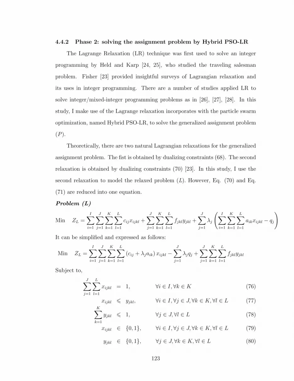
4.4.2 Phase 2: solving the assignment problem by Hybrid PSO-LR

The Lagrange Relaxation (LR) technique was first used to solve an integer

programming by Held and Karp [24, 25], who studied the traveling salesman

problem. Fisher [23] provided insightful surveys of Lagrangian relaxation and

its uses in integer programming. There are a number of studies applied LR to

solve integer/mixed-integer programming problems as in [26], [27], [28]. In this

study, I make use of the Lagrange relaxation incorporates with the particle swarm

optimization, named Hybrid PSO-LR, to solve the generalized assignment problem

(P).

Theoretically, there are two natural Lagrangian relaxations for the generalized

assignment problem. The fist is obtained by dualizing constraints (68). The second

relaxation is obtained by dualizing constraints (70) [23]. In this study, I use the

second relaxation to model the relaxed problem (L). However, Eq. (70) and Eq.

(71) are reduced into one equation.

Problem (L)

Min ZL =I∑i=1

J∑j=1

K∑k=1

L∑l=1

cijxijkl +J∑j=1

K∑k=1

L∑l=1

fjklyjkl +J∑j=1

λj

(I∑i=1

K∑k=1

L∑l=1

aikxijkl − qj

)It can be simplified and expressed as follows:

Min ZL =I∑i=1

J∑j=1

K∑k=1

L∑l=1

(cij + λjaik)xijkl −J∑j=1

λjqj +J∑j=1

K∑k=1

L∑l=1

fjklyjkl

Subject to,

J∑j=1

L∑l=1

xijkl = 1, ∀i ∈ I,∀k ∈ K (76)

xijkl 6 yjkl, ∀i ∈ I,∀j ∈ J,∀k ∈ K, ∀l ∈ L (77)K∑k=1

yjkl 6 1, ∀j ∈ J,∀l ∈ L (78)

xijkl ∈ {0, 1}, ∀i ∈ I,∀j ∈ J,∀k ∈ K, ∀l ∈ L (79)

yjkl ∈ {0, 1}, ∀j ∈ J,∀k ∈ K, ∀l ∈ L (80)

123

Problem L(λ) is a lower bound on the optimal objective function value of the

original problem (P) for any value of the Lagragian multiplier λ. To obtain the

highest lower bound, I would need to solve the following optimization problem [29].

L∗ = maxλ>0

L(λ) (81)

It is worth noting that the Lagrangian multipliers now are restricted to be

nonnegative. This is a necessary condition for holding of Z∗L(λ) 6 Z∗P where Z∗m is

the optimum value of problem m. This relaxation problem named a 0-1 generalized

upper bound problem. If there are no other side constraints, the problem is easily

solved in time proportional to |IJ | by determining mini(cij + λiaik).

The major task in deriving a good lower bound using the Lagrange method

is computing a good set of multipliers. Theoretically, the Lagrangian multiplier

problem can be solved by applying a linear programming methodology. One re-

sulting algorithm, is known as Dantzig-Wolf decomposition or generalized linear

programming. However, the expensive computational time is one of the major

disadvantage of this approach. Accordingly, a subgradient optimization method is

used to solve the Lagrangian multiplier problem [23]. Given an initial multiplier

vector λ, a sequence of multipliers is generated using the following equation:

λt+1 =[λt +4t(AX t −Q)

]+(82)

where X t is an optimal solution to L(λt) which is the Lagrangian problem with

multiplier vector λt and 4t is positive scalar step size. As mentioned above,

Eq.(81), the Lagrangian multipliers is restricted to be nonnegative. Thus, the

update formula, Eq.(82), is expressed by the notation [y]+ denotes the “positive

part” of the vector “y”; that is, the ith component of [y]+ equals the maximum of

0 and yi.

Let’s consider the choice of step sizes, 4t. If the step size is too small, the

algorithm would become stuck at the current point and not converge; if it is too

124

large, the iterates λt might overshoot the optimal solution and perhaps even oscil-

late between two non-optimal solutions. Poljak [30] showed that ZL(λt) converges

to ZL(λ∗) if 4t → 0 and∑T

t=14t → ∞. Certainly, these conditions are difficult

to be satisfied and therefore the method is always used as a heuristic. Thus, in

this study, the step size 4t is given by

4t =αt (UB − L(λt))

‖ AX t −Q ‖2(83)

where αt is a constant that is generally set to 2 at iteration 1 and divided by 2

after a given number (5 for this study) of consecutive iterations have passed during

which the best known lower bound has not improved.

The lower bounds are obtained by solving problem (L) while the better upper

bound is solved by a methaheuristic, discrete PSO. This hybrid technique is known

as Metaboosting [28, 31, 32]. Additionally, there is a chance that the discrete

PSO may not provide a feasible solution. In such a case, a feasibility restoration

technique (i.e., repairing procedure) would be activated. A simple rule based on

the Knapsack problem (Turnpike Theorem) is used to restore feasibility [33]. The

feasibility restoration procedure is described in Table 18 and the second phase

procedure is described in Table 19.

4.4.3 Phase 3: sequencing customers within routes

In this phase, the total travel distance between customers is minimized. This

is done by applying a Traveling Salesman Problem (TSP) algorithm to sequence

the customers so as to minimize the total distance traveled between customers for

vehicle. There are a number of TSP algorithms. The exact TSP algorithms can

solve optimal solutions for a small sequencing problem while the heuristic TSP

algorithms yield near optimal solutions for a large sequencing problem. The so-

lution of this phase is an input of the first phase for next iteration. An identical

assignment configuration must obtain the same route configuration. This require-

125

Table 18. Feasibility restoration procedure

1. Set j = 02. Terminate check. If the termination criteria hold, then stop. The outcome is UB3. If vehicle j is not overload, then go to step 6;

else calculate aik/cij ∀k, ∀j which are assigned to j4. Sort aik/cij in decreasing order and assign index m = 0 . . .M5. Set L = 0 and m = 05.1 If L = L+ (aik)m 6 Q, then L = L+ (aik)m

else go to step 5.35.2 Assign (aik)m to a closet available capacity vehicle5.3 m = m+ 15.4 If m 6M then go to step 5.1; else go to next step6 j = j + 17 Go to step 2

Table 19. The second phase procedure

Input: cij cost matrix, route orientation vectorOutput: the feasible solution and the infeasible solution

1. Initialization(a) Set t1 = 0 (iteration counter)(b) Initiate λt1

2. Terminate Check. If the termination criteria hold, then stopThe outcome of the algorithm will be the feasible assignment solution(optimal solution) and the infeasible assignment solution (LB);else go to next step

3. Solve problem L(λt1) using CPLEX solver4. If the solution is a feasible solution then terminate the algorithm and the outcome

is the feasible assignment solution; else go to next step5. Solve λt1+1

5.1. Solve UB, set t2 = 0(a) Terminate Check. If the termination criteria hold, then stop

The outcome is the UB and go to step 5.2; else go to next step(b) Solve UB using discrete PSO(c) If the final solution from discrete PSO is not feasible

then apply the feasibility restoration rule; else go to next step(d) Set t2 = t2 + 1

5.2. Calculate 4t1 using Eq.(83)5.3. Calculate λt1+1 using Eq.(82)6. Set t1 = t1 + 17. Go to step 2

126

Table 20. Customer locations

Customer x-position y-position

1 -2.0 2.02 -4.0 -1.03 -2.0 -3.04 0.5 -5.05 4.0 -1.06 5.0 1.07 1.0 2.0

ment supports a learning ability of the particle swarm in order to move the route

orientation in the next iteration.

As a result, an exact TPS approach is needed. Unfortunately, the TSP is an

NP-complete problem. Thus, a heuristic approach is a candidate for this study. As

mentioned above, an identical route configuration of an assignment configuration

is needed. In this study, I make use of a myopic heuristic, named Nearest neighbor

heuristic [34] to determine the sequence of each vehicle.

4.5 Example simulation

This section describes the procedure of the Hybrid PSO-LR for the partitioned

vehicle of a multi commodity recyclables collection problem using an example as

shown in Fig.48. There are 7 customers, 3 product types, and two adjustable

partition vehicles with total capacity Q = 30. The customer locations and the

amount of product types need to be picked up are shown in Table 20 and Table 21,

respectively. The total amount of recyclable is 55. Thus, the minimum number of

required vehicles is⌈∑I=7

i=1

∑K=3k=1 aikQ

⌉=⌈5530

⌉= 2. Note that it is assumed that there

are no fixed costs in this example.

Initialization

The route orientations are randomly generated. Suppose the route orienta-

tions array is [−1.0 1.0 2.0 − 1.0]. One array is for one particle in the swarm.

127

Figure 48. Example Simulation

Table 21. Amount of recyclables to be picked up (aik)

Customer Recyclables Recyclables RecyclablesType 1 Type 2 Type 3

1 4 1 32 4 4 33 3 3 24 4 2 15 1 4 36 1 1 17 2 4 4

128

Figure 49. Route orientations

That means if 40 particles are needed, 40 arrays of the route orientation are gen-

erated. In this example, I would like to show only one particle in the swarm. The

array means the first route orientation is positioned at (−1.0, 1.0) and the second

route orientation is positioned at (2.0,−1.0). Fig. 49 shows the route orientations

of the array [−1.0 1.0 2.0 − 1.0].

Phase 1

By using Eq. (75), the allocating cost, cij, is shown as Table 22.

Phase 2

The mathmetical model of Problem (L) is constructed. The Lagrange multi-

plier array is also generated in this step. Suppose the initial Lagrange multiplier

array is λj = [0.8 0.8] where j ∈ {1, 2}.

129

Table 22. Distance between the route orientations and the customer locations (cij)

Customer Route RouteLocations orientation 1 orientation 2

1 2.83 5.592 6.31 7.893 6.31 5.844 7.84 5.155 8.09 3.896 9.68 6.477 3.06 3.16

Min ZL =I∑i=1

J∑j=1

K∑k=1

L∑l=1

(cij + λjaik)xijkl −J∑j=1

λjqj

Subject to,

J∑j=1

L∑l=1

xijkl = 1, ∀i ∈ I,∀k ∈ K

xijkl 6 yjkl, ∀i ∈ I,∀j ∈ J,∀k ∈ K, ∀l ∈ LK∑k=1

yjkl 6 1, ∀j ∈ J,∀l ∈ L

xijkl ∈ {0, 1}, ∀i ∈ I,∀j ∈ J,∀k ∈ K, ∀l ∈ L

yjkl ∈ {0, 1}, ∀j ∈ J,∀k ∈ K, ∀l ∈ L

Problem (L) is solved by CPLEX. The results is xijkl array where i ∈

{1, .., 7}, j ∈ {1, 2}, k ∈ {1, 2, 3}, and l ∈ {1, 2}. If a feasible solution obtained,

the procedure of phase 2 is done and the optimal solution is found. However, if

an infeasible solution obtained, the subgradient optimization procedure is called

in order to find a new Lagrange multiplier of the next iteration.

Subgradient optimization method

The solution array dimension is 1×84 in which each element contains a binary

number. The process of subgradient optimization is not different from that found

in the literature. However, the upper bound is obtained by using the discrete PSO

130

which is introduced in Chpater 3. Additionally, it uses the solution array as the

input. If the solution from the discrete PSO is infeasible, the feasible restoration

procedure is called. The main concept of the restoration procedure is not different

from a bin packaging algorithm in which the benefit in this case is the amount of

recyclables (aak) and the weight is the cost allocation (cij), see [33].

Phase 3

The last phase makes use of a simple heuristic TSP, Nearest neighbor algo-

rithm. The method of the route orientation array updating is same as the contin-

uous PSO. For example, the initial route orientation array is [−1.0 1.0 2.0 −1.0]

and velocity of this array is [0.2 − 0.1 − 1.0 0.5]. The new route orientation

array for the next iteration is [−0.8 0.9 1.0 − 0.5]. The procedure of pbest and

gbest memorization is same as the standard process PSO.

4.6 Computational Experiments

To evaluate the performance of Hybrid PSO-LR algorithm, computational

experiments have been conducted on randomly generated instances. The proposed

algorithm has been compared to the sweep algorithm—as described in Section

3.4.2—and the discrete PSO, proposed in Chapter 3. Additionally, a Parallel

Particle Swarm Optimization (PPSO) algorithm is presented. The algorithms are

described in Section 4.6.2.

4.6.1 Test problems design

The number of customers was varied from 50 to 260 for the test problems while

the number of vehicles that was used to pick up recyclables was varied between 2

and 5. The total number of product types was varied between 2 and 5.

The instances are also divided into 3 series, 10 instances each. The first

series, 100 series, is named “Remote Depot I”. This series of instances simulates a

131

Figure 50. Scatter plot of customer locations (Remote depot I)

recycling facility which located outside a county and is serving only that county; as

a result, the customers are located in the up-right quadrant. The second series, 200

series, is named “Central Depot”. These instances imitate a situation in which a

recycling facility located inside a county. As a result, the customers are located on

all quadrants and the depot is on the center. The third series, 300 series, is named

“Remote Depot II”. These instances simulate a situation in which a recycling

facility is serving clusters of customers (between 2 and 5 clusters). Fig. 50, Fig.

51, and Fig. 52 depict the configurations of 100 series, 200 series, and 300 series

instances, respectively.

4.6.2 Competitive algorithms

Two other competitive approaches were proposed. They are based on the dis-

crete PSO approach in Section 3.4.4. However, these have been coded for different

programming approaches: sequential and parallel.

132

Figure 51. Scatter plot of customer locations (Central depot)

Figure 52. Scatter plot of customer locations (Remote depot II)

133

Direct sequential PSO

In this version, the PSO was coded as serial process using a single central

processing unit.

Direct parallel PSO

There are a number of parallel genetic algorithms. Nevertheless, the parallel

PSO (PPSO) approaches are rare. Schutte [35] tested a coarse-grained paral-

lelization of PSO on multiple local minima—large-scale analytical test problems

with computationally cheap function evaluations and medium-scale biomechanical

system identification problems with computationally expensive function evalua-

tions. The results suggested that the PPSO yields a high performance under load-

balanced conditions; alternatively, an asynchronous implementation is suitable for

load-imbalanced conditions. Chang et al. [36] studied communication strategies

in order to improve parallel efficiency. Cui [37] made use of a synchronous PPSO

scheme to solve the design of electromagnetic absorbers. The synchronous PPSO

scheme updates the global optimum only after the fitness values of all particles have

been evaluated. In contrast to the synchronous scheme, the asynchronous PPSO

scheme updates the global optimum value after each objective function evaluation.

The authors compared the synchronous PPSO with a binary genetic algorithm and

a real-coded genetic algorithm. The results showed that PSO is simpler to code

than GAs, the PSO is competitive with other relatively complicated algorithms,

and PSO may be more efficient than GAs. Venter [38] made use of an asynchronous

PPSO solving a structural sub-optimization problem and an optimization design

problem of an aircraft’s wing, Boeing 767. Waintraub et al. [39] proposed a pecu-

liar PPSO, named Island PPSO to solve nuclear engineering problems: reactor core

design (CD) and fuel reload (FR) optimization. The experimental results showed

that Island PPSO outperformed a serial PSO and more efficient and robust than a

134

master-slave PPSO scheme. To the best of my knowledge, there is no an applica-

tion of PPSO to the vehicle routing problem; specifically, the partitioned vehicle

for recyclables collection problem.

In this study, use has been made of a standard synchronized PPSO. There

are two reasons for this. First, the standard synchronize PPSO is a simple scheme

which is easy to code. Second, the standard synchronized PPSO is suitable for the

proposed algorithm, SSS-APSO, in which all updates and the process of extinction

and offspring reproduction must be performed after the fitness values of all particles

have been evaluated.


All parameters for two direct PSO algorithms (sequential and parallel versions)

in this study were the same as set in chapter 2 of SSS-APSO. They were set as

follows: the number of particles, N = 40; the number of sub-swarms, S = 4; the

maximum number of iterations, T = 1000; the maximum inertia weight, ωmax =

0.7; the minimum inertia weight, ωmin = 0.3; the step size of the inertia weight,

4ω = 0.1; the cognitive and social factors, φ1 = φ2 = 0.2; the standard deviation,

σ = 0.1n where n is |IK|. The different parameter settings for Hybrid PSO-LR

were the maximum number of iterations of the route orientation procedure, T0 =

5; the maximum number of iterations of the Lagrange relaxation procedure, T1 =

20; the maximum number of iterations of the PSO for UB solving, T2 = 10. These

are shown in Fig. 46 and Table 19.

4.6.4 Computational results

The Hybrid PSO-LR algorithm and other two competitive discrete PSO ap-

proaches (sequential and parallel versions) were coded in Python language 2.7 and

the tests were executed on a Windows 7 Intel Xeon, 2.4 GHz processor with 64 GB

135

of RAM. The algorithms were independently executed 10 times for each instance,

and the best fitness values, the worst fitness values, and the average fitness values

of each approach were reported. Table 23 shows the results of all competitive algo-

rithms and Tabel 24 shows the average values of the results. The best performance

among competitive algorithms are highlighted in bold face. The Hybrid PSO-LR

approach dominates other competitive algorithms in all instances.

136

Table 23. Computational results

Problem Num. Num. Num. SweepFitness value (total distance)

Cust. Recy. Routes Algorithm Discrete PSO (sequential) Discrete PSO (parallel) Hybrid PSO-LR

types Best Best Worst Ave. Time Best Worst Ave. Time Best Worst Ave. Time(min) (min) (min)

vrpc100 76 2 2 3747.47 3690.55 3744.62 3704.91 4.43 2923.19 3211.54 3091.75 2.36 929.37 1132.46 1014.66 26.62vrpc101 133 2 5 6821.20 6771.28 6864.53 6826.46 8.18 6272.32 6492.54 6410.98 4.93 1802.27 2146.02 1949.98 54.16vrpc102 146 4 4 7676.63 7621.17 7713.34 7643.84 8.93 6601.94 6843.18 6758.43 5.93 1401.06 1727.23 1524.96 49.06vrpc103 154 3 3 8801.18 8555.00 8679.29 8636.52 8.67 7358.74 7566.22 7438.82 6.51 1649.23 1804.90 1731.97 55.12vrpc104 176 3 3 9038.75 8781.61 8881.26 8843.94 10.07 7676.81 8056.61 7950.26 8.67 1299.53 1809.63 1521.02 52.13vrpc105 182 3 3 10206.98 10155.55 10173.10 10177.01 12.16 8659.55 8859.81 8782.99 8.71 1690.07 2093.12 1950.77 68.16vrpc106 202 2 2 10752.28 10463.13 10588.55 10544.30 10.85 9380.50 9975.81 9757.19 10.30 1579.95 1915.24 1684.08 78.20vrpc107 207 3 3 11704.73 11642.90 11744.38 11715.96 11.42 10015.93 10363.08 10236.98 11.59 2123.89 2399.55 2238.22 82.11vrpc108 217 4 3 11530.75 11408.95 11493.12 11454.46 12.43 10695.14 10804.04 10747.54 11.95 1702.26 1894.63 1791.62 80.59vrpc109 256 3 4 13597.23 13473.17 13524.28 13496.40 15.20 12314.02 12464.40 12356.67 13.67 2093.73 2816.39 2443.03 106.10



137

Table 24. Computational results (average)

Problem Num. Num. Num. SweepFitness value (total distance)

Cust. Recy. Routes Algorithm Discrete PSO (sequential) Discrete PSO (parallel) Hybrid PSO-LR

types Average Average Average Average

vrpc100 76 2 2 3925.05 3704.91 3091.75 1014.66vrpc101 133 2 5 6975.32 6826.46 6410.98 1949.98vrpc102 146 4 4 7812.67 7643.84 6758.43 1524.96vrpc103 154 3 3 8945.21 8636.52 7438.82 1731.97vrpc104 176 3 3 9201.67 8843.94 7950.26 1521.02vrpc105 182 3 3 10363.22 10177.01 8782.99 1950.77vrpc106 202 2 2 10887.83 10544.30 9757.19 1684.08vrpc107 207 3 3 11812.33 11715.96 10236.98 2238.22vrpc108 217 4 3 11698.25 11454.46 10747.54 1791.62vrpc109 256 3 4 13702.80 13496.40 12356.67 2443.03



138

Figure 53. Relative percent deviation of the results

The performance of proposed approach can be easily observed by presenting

it as a relative percent deviation. In this study, the relative percent deviation is

calculated as:

% deviation = −(F − SS

)× 100 (84)

where S is the fitness value of the sweep algorithm, F is the the fitness value of

the PSO-based approaches. Line plot of the relative percent deviation is shown

in Fig. 53. The Hybrid PSO-LR provides the better relative percent deviation

between 60% and 80%. The direct sequential PSO provides the percentage devia-

tion between -5% and 8%. Generally, the direct parallel PSO performs better than

the sequential version. However, in case of the Remote Depot II (300 series), the

direct parallel PSO generates worse solutions. I discuss this issue in Section 4.6.7.

Fig. 54, Fig. 55, and Fig. 56 show the vrpc300 route configurations of the

base solution, direct sequential PSO, and Hybrid PSO-LR, respectively. In this

particular instance, there are three clusters of 123 customers. The total distance

of the sweep algorithm is 4775.28 while of the direct sequential PSO and Hybrid

139

Figure 54. A route configuration of the sweep algorithm solution (vrpc300)

PSO-LR are 8227.13 and 2475.19, respectively.

Fig. 57 and Fig. 58 shows the route orientations of vrpc301 and vrpc305,

respectively. The vrpc301 needs 2 vehicles to serve 124 customers in which lo-

cated in two clusters. In the figure, we can see that the route orientations were

randomly generated in the area of the lower cluster (“START” points). Then,

the route orientations iteratively moved along with the particle swarm optimiza-

tion mechanism to serve each cluster separately, the red one moved to the upper

cluster while the blue one moved to serve the lower cluster. Likewise, Fig. 58,

the trajectories of three route orientations demonstrated that even if they were

started close to each other (red one and green one), they moved to serve the cus-

tomer clusters separately. This behavior encourages the second phase (solving the

assignment problem) to generate a good solution by providing a good allocating

cost (cij) matrix.

140

Figure 55. A route configuration of the direct sequential PSO solution (vrpc300)

Figure 56. A route configuration of the PSO-LR solution (vrpc300)

141

Figure 57. The characteristic of route orientation (vrpc301)

Figure 58. The characteristic of route orientation (vrpc305)

142

4.6.5 The performance of Hybrid PSO-LR algorithm

It is worth noting that Hybrid PSO-LR algorithm is the one who provides

percent gap of each instance. The percent gap is defined by the following equation.

% Gap =

(UB − LB

UB

)× 100 (85)

where UB is the best upper bound found (i.e., the objective value of the best

feasible found so far, by PSO method), and LB is a lower bound on the optimal

objective function value ZL(λ) of the problem (L).

To investigate the performance of PSO which is embedded in the subgradient

method, a variant of Hybrid PSO-LR algorithm which removed PSO from the

subgradient method has been coded. In this study, hypothesis testing is used to

test the significance of differences between the algorithms. The null hypothesis,

H0, is the population mean of percent gap of Hybrid PSO-LR is not significantly

different from the population mean of percent gap of the sole Lagrange relaxation

method, and the alternative hypothesis, H1, is the population mean of percent gap

of Hybrid PSO-LR is significantly different from the population mean of percent

gap of the sole Lagrange relaxation method.

H0 : µ1 − µ2 = 0

H1 : µ1 − µ2 6= 0

The Hybrid PSO-LR and the sole Lagrange relaxation algorithms were re-

peatedly executed for 5 times on each instance. The results are shown in Table 25.

The decisions were made from the comparison between P-value and α, (α = 0.05).

Obviously, in Table 25, the Hybrid PSO-LR yielded better percent gaps. This

supports that PSO which is embedded in Lagrange relaxation improves the per-

formance of the approach.

143

Table 25. Significant difference testing

Problem Hybrid PSO-LR Lagrange Relaxation Hypothesis testing

(α = 0.05)

Ave. % gap Std. % gap Ave. % gap Std. % gap P-value H0 vs H1

vrpc100 4.79 1.78 10.52 3.55 0.023 Reject H0vrpc101 7.32 2.56 12.44 2.38 0.014 Reject H0

vrpc102 5.76 2.05 10.93 3.12 0.021 Reject H0

vrpc103 4.05 2.16 9.83 2.45 0.005 Reject H0

vrpc104 9.63 1.42 14.74 3.55 0.031 Reject H0

vrpc105 9.94 2.13 13.89 2.65 0.036 Reject H0

vrpc106 2.75 0.89 4.32 1.17 0.048 Reject H0

vrpc107 10.93 2.72 14.67 1.95 0.041 Reject H0

vrpc108 4.36 1.49 7.55 2.04 0.026 Reject H0

vrpc109 8.14 1.43 10.78 1.55 0.027 Reject H0

vrpc200 7.62 0.89 9.64 0.74 0.006 Reject H0

vrpc201 4.36 0.55 7.14 1.93 0.036 Reject H0

vrpc202 8.15 1.42 10.24 1.01 0.031 Reject H0

vrpc203 10.66 2.37 14.81 1.99 0.020 Reject H0

vrpc204 6.83 1.04 9.12 0.89 0.007 Reject H0

vrpc205 6.23 0.78 7.69 1.11 0.047 Reject H0

vrpc206 1.65 1.04 4.73 1.86 0.018 Reject H0

vrpc207 7.82 1.51 10.04 1.32 0.043 Reject H0

vrpc208 8.93 1.26 12.17 2.41 0.037 Reject H0

vrpc209 10.21 1.73 14.99 2.86 0.019 Reject H0

vrpc300 4.73 1.34 6.80 1.18 0.036 Reject H0

vrpc301 7.09 0.46 8.81 1.12 0.025 Reject H0

vrpc302 8.15 1.47 10.22 1.28 0.049 Reject H0

vrpc303 11.31 2.17 16.65 2.88 0.013 Reject H0

vrpc304 3.78 2.64 8.09 2.16 0.026 Reject H0

vrpc305 7.13 1.11 9.40 1.27 0.020 Reject H0

vrpc306 10.15 1.08 15.76 1.79 0.001 Reject H0

vrpc307 9.14 2.30 12.82 2.23 0.037 Reject H0

vrpc308 6.91 2.02 9.84 1.78 0.045 Reject H0

vrpc309 7.69 1.05 9.41 0.84 0.024 Reject H0

144

Figure 59. Regression analysis of problem size and computational time

4.6.6 Analysis of the computational time

Inevitably, the high performance of Hybrid PSO-LR costs us a high computa-

tional time. As in Table 23, Hybrid PSO-LR took almost 2 hours for the problem

size with 1245 decision variables (vrpc309: 251 customers × 4 recyclable types)

and at least 25 minutes for a small problem (vrpc100: 76 custmers × 2 recyclable

types = 152 decision variables). It is about 6 times more than the direct sequential

PSO algorithm and about 8 times more than the direct parallel PSO algorithm.

Fortunately, it can be shown that the computational time of the proposed algo-

rithm can be formulated as linear function of problem size (in another word, a

polynomial time with the highest power 1). Fig. 59 is the regression analysis from

Minitab with 300 data points from Table 23. It is suggests that the possible linear

function is,

CT = 17.30 + (0.0085×NP ) (86)

where CT is the computational time (min.) and NP is the problem size. Fig. 60

shows the fitted line plot of Hybrid PSO-LR’s computational time versus problem

size. Even the coefficient of determination (R2) is not large (65.0%), it is clear that

the line should not be an exponential function. The residual plots are depicted as

in Fig. 61.

145

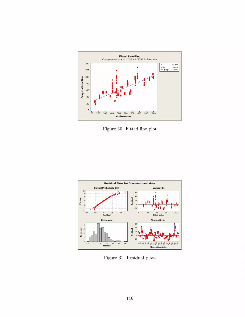
Figure 60. Fitted line plot

Figure 61. Residual plots

146

Figure 62. Customer locations of vrpc309: I = 251

4.6.7 Analysis of the performance of the direct parallel PSO

The direct parallel PSO dominated the direct sequential PSO in cases of Re-

mote Depot I and Central Depot. However, the parallel version’s performance was

worse than the sequential version’s performance in case of Remote Depot II. In

this section, an analysis of problem vrpc309 that has 251 customers and 4 product

types has been conducted. Fig. 62 shows the customer locations; Q1, Q2, Q3, and

Q4 denote a quadrant 1, 2, 3, and 4, respectively.

Test 1

To investigate an effect of the number of customers, the number of customers

in problem vrpc309 were randomly reduced by 50% and 75%. Thus, there were

121 customers in the first case in which located as the same configuration of the

original vrpc309, see Fig. 63. Likewise, there were 55 customers in the second

case, see Fig. 64. The vehicle capacity was also modified by reducing by half in

order to observe the effect. The direct sequential PSO and the direct parallel PSO

were executed 5 times on each test cases. The results, mean optimal solution, are

147

Figure 63. Customer locations of modified vrpc309: I = 121

Table 26. The effect of problem size

Problem 100% vehicle capacity 50% vehicle capacitySequential Parallel Sequential Parallel

vrpc309-c121 4675.06 9053.93 4803.94 10027.14vrpc309-c55 2349.66 3202.94 2333.36 3407.94

shown in Table 26

It is clear that the problem size was not the factor which degraded the per-

formance of direct parallel PSO. The sequential version outperformed the parallel

version at both modified vrpc309. The critical factor may be customer locations

in clusters.

Test 2

In this test, the instance is tested by area. That is each quadrant was examined

separately: Q1, Q2, Q3, and Q4. Then, its combinations were tested: Q1Q2,

Q2Q3, Q3Q4, Q1Q4, and Q1Q2Q3. Additionally, the variations of the vehicle

capacity were tested as Test 1. The mean optimal values are shown in Table 27.

As seen in the results, results of the direct parallel PSO was still lagging those

148

Figure 64. Customer locations of modified vrpc309: I = 55

Table 27. The effect of customer locations

Problem Number of 100% vehicle capacity 50% vehicle capacityvrpc309 customers Sequential Parallel Sequential ParallelQ1 90 3120.89 3531.87 3214.09 3374.55Q2 61 1862.69 1758.32 2048.93 1744.11Q3 37 1347.13 854.58 1325.30 862.27Q4 63 2674.09 2345.79 2763.30 2432.39Q1Q2 151 5248.93 8972.63 5430.41 9689.98Q2Q3 98 3663.73 4231.38 3747.24 4161.18Q3Q4 100 4144.35 6101.18 4224.40 5828.91Q1Q4 153 5881.98 9473.21 6090.36 9659.71Q1Q2Q3 188 7083.72 14061.74 7264.22 14222.32

149

of the sequential version. The characteristic of the customer locations is still in

clusters (even only one cluster). The parallel version could only provided better

solutions on small-size instances (below 90 customers). However, it was degraded

for the large-size instances.

In conclusion, the direct parallel PSO has a fast convergence rate. It shows

a high performance on both quality of the solutions and low computational cost.

Nonetheless, its performance is degraded when customers are clustered. In other

words, the direct parallel PSO tends to converge prematurely on a local optimum

and it is easily entrapped on a multi-local optima problem in such case. However,

a definitive conclusion has not been achieved on this issue, it is left as an opened

problem because the issue is beyond the scope of this study.

4.6.8 Effect of the number of vehicles

In this study, the number of vehicles was set as a parameter. The number

must be determined by a practitioner. He/she may use a simple calculation to

find the minimum number of vehicles needed. Usually, it is calculated by solving

the Bin Package Problem (BPP) associated with the CVRP, which calls for the

determination of minimum number of bins (Lmin), each with capacity Q, required

to load all |IK| items, with each amount aik. The trivial BPP calculation is

expressed as follows:

Lmin =

⌈∑Ii=1

∑Kk=1 aik

Q

⌉(87)

Definitely, there is nothing guaranteed that Lmin would return the minimum

total travel distance. Accordingly, the work is left to a practitioner to make the

decision. Suppose a recycling company has a big enough fleet of vehicles (i.e.,

there is no fixed cost), it is a good practice to compare the fitness value obtain

by different number of vehicles. Fig. 65, Fig. 66, and Fig. 67 present trends of

the optimal solutions influenced by the number of vehicles of some 100 series, 200

150

Figure 65. Optimum value and number of vehicles (100 series)

series, and 300 series instances, respectively. Note that Lmin = 4 for all instances.

It is clear that the Lmin of each instance had not yielded the minimum fitness

value. For example, Fig. 65, the minimum fitness value occurs when the number

of vehicles are 6, 5, and 5 for vrpc103, vrpc105, and vrpc109, respectively. It is

recommended that a practitioner try out some number of vehicles above Lmin

4.7 Conclusions and Further Research Directions

In this chapter, a combined heuristic and metaheuristic algorithm has been

developed to solve an NP-hard problem, the partitioned vehicle for a multi com-

modity recyclables collection problem. The problem was formulated as the general

assignment problem and solved by a Lagrangian relaxation technique as proposed

by Mohanty [1]. However, the key differences are that the assignment cost have

been calculated as insertion costs with a route orientation and the route orienta-

tion was iteratively moved by the particle swarm optimization. The next difference

is the Lagrange relaxation was embedded by the particle swarm optimization in

order to find a promising upper bound in the process of subgradient technique.

151



152

This kind of technique is known as “Metaboosting”.

The performance of the proposed method was evaluated on generated in-

stances. The results showed that the Hybrid PSO-LR yielded promise solutions in

all instances. It also provided good lower bounds. The computational time does

increased; nevertheless, it has been demonstrated that the computational time is

governed by the problem size as a linear function.

This study has also been extended on a parallel PSO (PPSO). The direct

parallel PSO worked well on specific forms of customer locations: the Remote

depot I and the Central depot for this study. Unfortunately, the approach did not

work well in case of the Remote depot II (clusters of customer locations). From

the analysis, Section 4.6.7, it showed that the size of the problems is not the cause.

A possible cause is the configuration of customer as clusters. The solution of this

problem is beyond the scope of this study, and is left for future study.

153

List of References

[1] N. Mohanty, “A multi commodity recyclables collection model using parti-tioned vehicles,” Ph.D. dissertation, University of Rhode Island, 2005.

[2] J. R. Stock, “Reverse logistics,” Oak Brook, IL, Tech. Rep., 1992.

[3] D. S. Rogers and Tibben-Lembke, Going Backwards: Reverse Logistics Trendsand Practices. Pittsburgh, PA, USA: Reverse Logistics Executive Council,1999.

[4] M. Fleischmann, “Quantitative models for reverse logistics,” Ph.D. disserta-tion, Erasmus University Rotterdam, 2000.

[5] M. Fleischmann, J. M. Bloemhof-Ruwaard, R. Dekker, E. van der Laan, J. A.van Numen, and L. N. V. Wassenhove, “Quantitative models for reverse logis-tics: a review,” European Journal of Operational Research, vol. 103, pp. 1–17,1997.

[6] S. Seuring and M. Muller, “From a literature review to a conceptual frameworkfor sustainable supply chain management,” Cleaner Production, vol. 16(15),pp. 1699–1710, 2008.

[7] M. Brandenburg, K. Govindan, J. Sarkis, and S. Seuring, “Quantitative mod-els for sustainable supply chain management: developments and directions,”European Journal of Operational Research, vol. 233(2), pp. 299–312, 2014.

[8] E. de Oliveira Simonetto and D. Borenstein, “A decision support systemfor the operational planning of solid waste collection,” Waste Management,vol. 27, pp. 1286–1297, 2007.

[9] V. N. Bhat, “A model for the optimal allocation of trucks for solid wastemanagement,” Waste Management & Research, vol. 14, pp. 87–96, 1996.

[10] F. McLeod and T. Cherrett, Waste: a Handbook for Management. Burling-ton, MA: Academic Press, 2011, ch. Wasre Collection, pp. 61–73.

[11] B. Reimer, M. Sodhi, and V. Jayaraman, “Truck sizing models for recyclablespick-up,” Computers & Industrial Engineering, vol. 51, pp. 621–636, 2006.

[12] H. Wiese and S. Zelewski, “Waste disposal and waste avoidance,” Interna-tional Journal of Production Research, vol. 40, pp. 3391–3400, 2002.

[13] B. G. Wilson and B. W. Baetz, “Modeling municipal solid waste collectionsystems using derived proability distribution i: modeling development,” En-vironmental Engineering, vol. 127(11), pp. 1031–1038, 2001.

154

[14] B. G. Wilson and B. W. Baetz, “Modeling municipal solid waste collectionsystems using derived proability distribution i: extensions and applications,”Environmental Engineering, vol. 127(11), pp. 1039–1047, 2001.

[15] E. D. Chajakis and M. Guignard, “Scheduling deliveries in vehicle with mul-tiple compartments,” Global Optimization, vol. 26, pp. 43–78, 2003.

[16] P. Avella, M. Boccia, and A. Sforza, “Solving a fuel delivery problem byheuristic and exact approaches,” European Journal of Operational Research,vol. 152, pp. 170–179, 2004.

[17] F. Cornillier, F. Boctor, G. Laporte, and J. Renaud, “An exact algorithmfor the petrol station replenishment problem,” Operational Research Society,vol. 59, pp. 607–615, 2008.

[18] A. E. Fallahi, C. Prins, and R. W. Calvo, “A memetic algorithm and a tabusearch for the multi-compartment vehicle routing problem,” Computers &Operations Research, vol. 35, pp. 1725–1741, 2008.

[19] L. Muyldermans and G. Pang, “On the benefits of co-collection: experimentswith a multi-compartment vehicle routing algorithm,” Euroupean Journal ofOperational Research, vol. 206, pp. 93–103, 2010.

[20] J. Melechovsky, “Evolutionary local search algorithm to solve the multi-compartment vehicle routing problem with time windows,” in Proceedings of30th International Conference on Mathematical Methods in Economics, 2012,pp. 564–568.

[21] M. Reed, A. Yiannakou, and R. Evering, “An ant colony algorithm for themulti-compartment vehicle routing problem,” Applied Soft Computing, vol. 15,pp. 169–176, 2014.

[22] U. Derigs, J. Gottlieb, J. Kalkoff, M. Piesche, F. Rothlauf, and U. Vogel,“Vehicle routing with compartments: applications, modelling and heuristics,”OR Spectrum, vol. 33(4), pp. 885–914, 2011.

[23] M. L. Fisher, “The lagrangian relaxation method for solving integer program-ming problem,” Management Science, vol. 27(1), pp. 1–18, 1981.

[24] M. Held and R. M. Karp, “The traveling salesman problem and minimumspanning trees,” Operations Research, vol. 18(6), pp. 1138–1162, 1970.

[25] M. Held and R. M. Karp, “The traveling salesman problem and minimumspanning trees, part ii,” Mathematical Programming, vol. 1(1), pp. 6–25, 1971.

[26] R. Sridharan, “A lagrangian heuristic for the capacitated plant location prob-lem with side constraints,” Operational Research Society, vol. 42(7), pp. 579–585, 1991.

155

[27] V. Jeet and E. Kutanoglu, “Lagrangian relaxation guided problem spacesearch heuristics for generalized assignment problems,” European Journal ofOperational Research, vol. 182, pp. 1039–1056, 2007.

[28] M. Leitner and G. R. Raidl, “Lagrangian decomposition, metaheuristics, andhybrid approaches for the design of the last mile in fiber optic networks,”Hybrid Metaheuristics, vol. 5296, pp. 158–174, 2008.

[29] R. K. Ahuja, T. L. Magnanti, and J. B. Orlin, Network Flows, 1st. edn. NewJersey, USA: Prentice-Hall, 1993.

[30] B. Poljak, “Minimization of unsmooth functionals,” USSR ComputationalMathematics and Mathematical Physics, vol. 9(3), pp. 14–29, 1969.

[31] C. Blum and A. Roli, Hybrid Metaheuristics. New York, USA: Springer,2008, ch. Hybrid Metaheuristics: An Introduction, pp. 1–30.

[32] J. Puchinger, G. R. Raidl, and S. Pirkwieser, Hybridizing Metaheuristics andMathematical Programming. New York, USA: Springer, 2010, ch. Mata-boosting: Enhancing Integer Programming Techniques by Metaheuristics, pp.71–102.

[33] W. L. Winston and M. Venkataramanan, Introduction to Mathematical Pro-gramming, 4th. edn. Pacific Grove, CA, USA: Thomson, 2003.

[34] S. Chopra and P. Meindl, Supply Chain Management, 2nd. edn. New Jersey,USA: Pearson Prentice Hall, 2004.

[35] J. F. Schutte, J. A. Reinbolt, B. J. Fregly, R. T. Haftka, and A. D. George,“Parallel global optimization with the particle swarm algorithm,” Interna-tional Jouranl for Numerical Methods in Engineering, vol. 61, pp. 2296–2314,2004.

[36] J. Chang, S.-C. Chu, J. F. Roddick, and J.-S. Pan, “A parallel particle swarmoptimization algorithm with communication strategies,” Information Scienceand Engineering, vol. 21(4), pp. 809–818, 2005.

[37] S. Cui and D. S. Weile, “Applicaiton of a parallel particle swarm optimizationscheme to the design of electromagnetic absorbers,” IEEE Transaction onAntennas and Propagation, vol. 53(11), pp. 3616–3624, 2005.

[38] G. Venter and J. Sobieszczanski-Sobieski, “A parallel particle swarm optimiza-tion algorithm accelerated by asynchronous evaluations,” Aerospace Comput-ing, Information, and Communication, vol. 3(3), pp. 123–137, 2006.

[39] M. Waintraub, R. Schirru, and C. M. Pereira, “Multiprocessor modeling ofparallel particle swarm optimization applied to nuclear engineering problems,”Progress in Nuclear Energy, vol. 51, pp. 680–688, 2009.

156

CHAPTER 5

Conclusions

The Vehicle Routing Problem (VRP) is a well known NP-hard problem. It

has been solved by a number of exact algorithms for decades; however, the ex-

act algorithms—parallel branch-and-cut-and-price, for example—are able to solve

an instance involving fewer than 100 customers. In practice, several heuris-

tic/metaheuristic methods have been used to solve industry-size vehicle routing

problems (medium/large-size problems) to obtain near optimal solutions in a rea-

sonable amount of time.

This research started with an exploration of an Evolutionary Computation

technique, Particle Swarm Optimization (PSO). Then, two novel PSO-based algo-

rithms has been proposed—Survival Sub-swarms Adaptive PSO (SSS-APSO) and

Survival Sub-swarms Adaptive PSO with velocity-line bouncing (SSS-APSO-vb).

The computational experiments showed that both proposed methods outperformed

the existing algorithms in literature. Specifically, the SSS-APSO works well on the

unimodal landscapes, while the SSS-APSO-vb works well on the multimodal land-

scapes. As previously stated, the SSS-APSO is a special case the SSS-APSO-vb

when δ = 1. A practitioner may vary the δ in favor of obtaining the best solution

in a case of the characteristic of a function is unknown. It is worth noting that

the global search (i.e., exploration) is enhanced by the sub-swarms and velocity-

line bouncing methods; on the other hand, the local search (i.e., exploitation) is

enhanced by the classical swarm topology.

Two simple solution representations—continuous and discrete—for the CVRP

were discussed in Chapter 3. The resolution procedure was a combination of SSS-

APSO-vb and common local improvement methods. Two well-known benchmark

157

data sets were used to test the performance compared to other competitive PSO-

based approaches. The experiment results showed that the proposed PSOs ob-

tained solutions comparable to the best known solutions. Precisely, the continu-

ous PSO worked well on the small-size problems (n 6 75), while the discrete PSO

outperforms other algorithms on the large-size problems (n > 75). A key factor of

the discrete PSO is the noisy-fitness evaluation which enhances the global search

of the particle. However, the noise can be controlled by σ which is a practitioner’s

choice.

Finally, the application of the SSS-APSO for the partitioned vehicle of a multi

commodity recyclables collection problem was described in Chapter 4. The prob-

lem was formulated as a general assignment problem (GAP). The allocating cost

was calculated as an insertion cost method and the route orientation was positioned

by the SSS-APSO method. The GAP was solved by the Lagrange Relaxation tech-

nique in which the Lagrange Multiplier vector was solved by subgradient method.

Furthermore, the step sizes of the subgradient method was embedded by the SSS-

APSO in order to find a better upper bound. The procedure used in this problem

is named as Hybrid Particle Swarm Optimization-Lagrange Relaxation (Hybrid

PSO-LR). This kind of combining method is known as Metaboosting. The ran-

domly generated instances were simulated in a favor of testing the performance of

Hybrid PSO-LR. The results of case simulation showed that the Hybrid PSO-LR

outperformed the discrete PSO in which using the discrete solution representation

in Chapter 3.

In the future, the parallel PSO (PPSO) needs to be studied in more detail.

The computational time for a large-scale problem is a problem in practice. PPSO is

one of alternatives to cope with this problem. However, the knowledge of PPSO is

still limited. The behavior of the particles when proceeded in parallel programming

158

are not clear yet. As shown in Chapter 4, the parallel PSO has fast convergence

rate, but the solution’s quality degrades when customers are clustered. Thus, all

aspects relevant to PPSO should be studied and applied to the vehicle routing

problem and/or other optimization problems.

159

APPENDIX A

Analysis of Convergence

Van den Bergh [1] gave the convergence definition of PSO, stated as follows.

Definition 1. Given a particle position x(t) and an arbitrary position p in search

space, the convergence is defined as

limt→∞

x(t) = p (A.1)

It implies that the particle stops at a certain point p in search space. van

den Bergh also analyzed the trajectories of particles. He concluded that all the

particles are convergent to the positions of the global best solutions. That means

the whole swarm is influenced by the gbest. However, the gbest itself changes the

position as the process evolves. Thus, we need the second definition in order to

state that the PSO algorithm has achieved convergence.

Definition 2. Given that the best position of PSO in time t or in rth generation

is gbest(t), gbest∗ is a fixed position in search space, the convergence definition is

written as,

limt→∞

gbest(t) = gbest∗ (A.2)

The second definition implies that, if gbest output by PSO does not change,

then convergence is achieved. If the gbest is the global optimum solution, then

the algorithm attains the global optimum convergence. Otherwise, the algorithm

is stuck in local optima. We shall consider the analysis as the studies of [1, 2, 3, 4]

Without loss of generality, we will consider one-particle one-dimensional classic

PSO algorithm. Assume θ = θ1+θ2 = φ1β1+φ2β2 and (0 ≤ θ ≤ 4). It is reasonable

to assume that after a number of generations of the algorithm, p and pg are constant

160

numbers (a fixed-position particle). Thus, Eq. (15) and (8)can be written as,

vt+1 = ωvt − θxt + θ1p+ θ2pg (A.3)

xt+1 = (1− θ)xt + ωvt + θ1p+ θ2pg (A.4)

Accordingly, we can get

xt+2 = ω(xt+1 − xt) + (1− θ)xt+1 + Θ (A.5)

where Θ = θ1p+ θ2pg. By simplifying Eq. (A.5), we can get

xt+2 + (θ − ω − 1)xt+1 + ωxt = Θ (A.6)

Furthermore, the second derivative characteristic equation can be described by

λ2 + (θ − ω − 1)λ+ ω = 0 (A.7)

Accordingly, the corresponding eigenvalues of above equation are

λ1,2 =1 + ω − θ ±

√∆

2(A.8)

where ∆ = (θ − ω − 1)2 − 4ω. Under the condition of ∆ ≥ 0, we can get

ω ≤ θ + 1− 2√θ or ω ≥ θ + 1 + 2

√θ (A.9)

On the other hand, under the condition of ∆ < 0, the relationship between ω and

θ is

θ + 1− 2√θ < ω < θ + 1 + 2

√θ (A.10)

Convergence characteristic

We shall consider the eigenvalues in two cases: real numbers, complex num-

bers.

161

Case 1. −1 < λ1 ≤ λ2 < 1 (real number). From the knowledge of linear system,

all particles approach to convergent if λ1 and λ2 smaller than 1. Firstly, consider

λ1 > 1. We can get

1 + ω − θ −√

(θ − ω − 1)2 − 4ω

2> −1 (A.11)

ω − θ + 3 >√

(θ − ω − 1)2 − 4ω (A.12)

Concisely, the corresponding relationship between ω and θ is{ω > θ − 32ω − θ + 2 > 0

(A.13)

Secondly, considering λ2 < 1, we can obtain

1 + ω − θ +√

(θ − ω − 1)2 − 4ω

2< 1 (A.14)√

(θ − ω − 1)2 − 4ω < θ − ω + 1 (A.15)

As a result, we can get

ω < 1 + θ (A.16)

From (A.10), (A.13), and (A.16), the relationship between inertia weight and θ on

real eigenvalue can be summarized as{ω < θ + 1− 2

√θ

ω > θ2− 1

(A.17)

Case 2. λ1, λ2 are complex numbers under the condition of ∆ < 0. Thus, we can

obtain

∆ = (1 + ω − θ)2 − 4ω < 0 (A.18)

θ + 1− 2√θ < ω < θ + 1 + 2

√θ (A.19)

The sum of squares of the real part and the imaginary part is strictly smaller than

1, and then we have

(ω + 1− θ)2

4− (θ − ω − 1)2

4< 1 (A.20)

ω < 1 (A.21)

162

According to (A.17) and (A.21), the corresponding result between ω and θ can be

summarized as

θ + 1− 2√θ < ω < 1 (A.22)

From (A.17) and (A.22), convergence condition of the simplified PSO algorithm isω < 1ω > θ

2− 1

θ > 0(A.23)

Divergence characteristic

If and only if key parameters, which mainly consist of ω and θ, are strictly

subjected to the conditions of |λ1| > 1 and |λ2| > 1, the particles finally have the

divergence behavior.

Firstly, under the conditions of λ1 > 1 and ∆ > 0, the corresponding diver-

gence region can be expressed as

ω > 1 + θ + 2√θ (A.24)

Secondly, under the conditions of λ2 < −1 and ∆ > 0, we can obtain

0.5× θ − 1 < ω < θ − 3 (A.25)

Thirdly, under the condition of ∆ < 0, the corresponding region of divergence

behavior is

1 < ω < 1 + θ + 2√θ (A.26)

According to (A.22)-(A.24), when both absolute eigenvalues are strictly larger than

1, the particles finally have the divergence behavior and the corresponding region

in θ ∈ (0, 4) can be conducted by

ω > 1 (A.27)

163

Figure A.1. The convergent and divergent regions

If and only if one absolute is strictly larger than 1 and the other absolute eigenvalue

is strictly smaller than 1, the particles also have divergence behavior and the

corresponding region in θ ∈ (0, 4) can be summarized as

ω <θ

2− 1 (A.28)

The area of convergence/divergence is shown in Fig. A.1.

164

List of References

[1] F. van den Bergh, “An analysis of particle swarm optimizers,” Ph.D. disserta-tion, University of Pretoria, 2001.

[2] J. Liu, X. Ren, and H. Ma, “A new pso algorithm with random c/d switchings,”Applied Mathematics and Computation, vol. 218, pp. 9579–9593, 2012.

[3] Y. Jiang, T. Hu, C. Huang, and X. Wu, “An improved particle swarm optimiza-tion algorithm,” Applied Mathematics and Computation, vol. 193, pp. 231–239,2007.

[4] I. C. Trelea, “The particle swarm optimization algorithm: convergence analysisand parameter selection,” Information Processing Letters, vol. 85, pp. 317–325,2003.

165

APPENDIX B

Multi-Valued Discrete PSO

Osadciw and Veeramachaneni [1] concluded the discrete multi-valued opti-

mization problems in which the range of variable lie between 0 and M − 1, where

M implies an M -ary number system. The same velocity update and particle rep-

resentation are used in the algorithm. The position update equation is, however,

change as follows.

1. Transform the velocity using

Sid =M

1 + e−vid(B.1)

2. A number is the generated using a normal distribution with µ = Sid and σ as

parameters

Xid = round(Sid + (M − 1)× σ × rand(1)) (B.2)

3. The number is rounded to the closet discrete variable with the end points fixed

If Xid > M − 1 then Xid = M − 1 (B.3)

and If Xid < 0 then Xid = 0 (B.4)

4. The velocity update equation remains the as Eq. (45). 5. The positions of

particles are discrete values between 0 and M − 1.

Probability of a discrete value m : For a given µ, a number is generated

using a normal distribution with the meant as µ and standard deviation σ for an

M-ary system. Based on this normal distribution and Eq. (B.3), the probability

for a specific discrete variables given µ can be calculated based on the area under

that region of the Gaussian curve. For a Sid, the probability of a discrete variable

166

having a value m is given by: m = 0

P (Xid = 0|Sid) =

∫ 0.5

−∞g(x)dx

= 1−Q(

0.5− Sidσ(M − 1)

)(B.5)

where Q is the error function. The function g(x) is

g(x) =1√

2πσ2(M − 1)2exp

(−1

2σ2(M − 1)2(x− Sid)

)(B.6)

with m in the range 1 to M − 2, the conditional probability of achieving Xid given

a previous Sid value is

P (Xid = m|Sid) =

∫ m−0.5

m+0.5

g(x)dx

= Q

(m− 0.50Sidσ(M − 1)

)−Q

(m+ 0.5− Sidσ(M − 1)

)(B.7)

For m = M − 1, the conditional probability is

P (Xid = (M − 1)|Sid) =

∫ ∞(M−1)−0.5

g(x)dx

= Q

((M − 1)− 0.5− Sid

σ(M − 1)

)(B.8)

Note that

M∑m=0

P (Xid = m/Sid) = 1 (B.9)

One can significantly control the performance of the algorithm using these

equations. For example, controlling the σ controls the standard deviation of the

Gaussian and, hence, the probabilities of various discrete variables.

167

List of References

[1] L. Osadciw and K. Veeramachaneni, Particle Swarm Optimization. Vienna,Austria: In-Tech, 2009, ch. Particle Swarms for Continuous, Binary, and Dis-crete Search Spaces, pp. 451–460.

168

BIBLIOGRAPHY

Agarwal, Y., Mathur, K., and Salkin, H. M., “A set-partitioning-based exact al-gorithm for the vehicle routing problem,” Networks, vol. 19(7), pp. 731–749,1989.

Ahuja, R. K., Ergun, O., Orlin, J. B., and Punnen, A. P., “A survey of verylarge-scale neighborhood search techniques,” Discrete Applied Mathematics,vol. 123, pp. 75–102, 2002.

Ahuja, R. K., Magnanti, T. L., and Orlin, J. B., Network Flows, 1st. edn. NewJersey, USA: Prentice-Hall, 1993.

Ai, T. J. and Kachitvichyanukul, V., “A study on adaptive particle swarm opti-mization for solving vehicle routing problem,” in Proceedings of the 9th AsiaPacific Industrial Engineering & Management Systems Conference, 2008, pp.2262–2268.

Ai, T. J. and Kachitvichyanukul, V., “Particle swarm optimization and two so-lution representations for solving the capacitated vehicle routing problem,”Computers & Industrial Engineering, vol. 56, pp. 380–387, 2009.

Ai, T. J. and Kachitvichyanukul, V., “A particle swarm optimization for the ve-hicle routing problem with simultaneous pickup and delivery,” Computers &Operations Research, vol. 36, pp. 1693–1702, 2009.

Al-kazemi, B., “Multi-phase generalization the particle swarm optimization algo-rithm,” in Proceedings of the 2002 Congress on Evolutionary Computation,2002.

Al-kazemi, B. and Mohan, C. K., “Multi-phase discrete particle swarm optimiza-tion,” in Proceedings of the Fourth Internation Workshop on Fromtiers inEvolutionary Algorithms, 2000.

Antonsson, E. K., Zhang, Y., and Martinoli, A., “Evolving engineering designtrade-offs,” in Proceedings of the ASME Fifteenth International Conferenceon Design Theory and Methodology, 2003.

Avella, P., Boccia, M., and Sforza, A., “Solving a fuel delivery problem by heuristicand exact approaches,” European Journal of Operational Research, vol. 152,pp. 170–179, 2004.

Baker, B. M. and Ayechew, M., “A genetic algorithm for the vehicle routing prob-lem,” Computers & Operations Research, vol. 30(5), pp. 787–800, 2003.

169

Baldacci, R., Mingozzi, A., and Roberti, R., “Recent exact algorithms for solvingthe vehicle routing problem under capacity and time window constraints,”European Journal of Operational Research, vol. 218, pp. 1–6, 2012.

Balinski, M. L. and Quandt, R. E., “On an integer program for a delivery problem,”Operations Research, vol. 12(2), pp. 300–304, 1964.

Banks, A., Vincent, J., and Anyakoha, C., “A review of particle swarm optimiza-tion. part 1: background and development,” Natural Computing, vol. 6, pp.467–484, 2007.

Banks, A., Vincent, J., and Anyakoha, C., “A review of particle swarm opti-mization. part 2: hybridisation, combinatorial, multicriteria and constrainedoptimization, and indicative applications,” Natural Computing, vol. 7, pp.109–124, 2008.

Belmecheri, F., Prins, C., Yalaoui, F., and Amodeo, L., “Particle swarm opti-mization algorithm for a vehicle routing problem with heterogeneous fleet,mixed backhauls, and time windows,” Intelligent Manufacturing, vol. 24, pp.775–789, 2013.

Beyer, H.-G., “Evolutionary algorithms in noisy environments: theoretical issuesand guidelines for practice,” Computer Methods in Mechanics and AppliedEngineering, vol. 186, pp. 239–267, 2000.

Bhat, V. N., “A model for the optimal allocation of trucks for solid waste man-agement,” Waste Management & Research, vol. 14, pp. 87–96, 1996.

Blum, C. and Roli, A., Hybrid Metaheuristics. New York, USA: Springer, 2008,ch. Hybrid Metaheuristics: An Introduction, pp. 1–30.

Bramel, J. and Simchi-Levi, D., “A location based heuristic for general routingproblems,” Operations Research, vol. 43(4), pp. 649–660, 1995.

Brandenburg, M., Govindan, K., Sarkis, J., and Seuring, S., “Quantitative mod-els for sustainable supply chain management: developments and directions,”European Journal of Operational Research, vol. 233(2), pp. 299–312, 2014.

Braysy, O. and Gendreau, M., “Vehicle routing problem wiht time windows, part i:route construction and local search algorithms,” Transportation Science, vol.39(1), pp. 104–118, 2005.

Breedam, A. V., “Improvement heuristics for the vehicle routing problem basedon simulated annealing,” European Journal of Operational Research, vol. 86,pp. 480–490, 1995.

170

Breedam, A. V., “Comparing descent heuristics and metaheuristics for the vehiclerouting problem,” Computers & Operations Research, vol. 28, pp. 289–315,2001.

Bullnheimer, B., Hartl, R. F., and Strauss, C., “An improved ant system algorithmfor vehicle routing problem,” Annals of Operations Research, vol. 89, pp. 319–328, 1999.

Bullnheimer, B., Hartl, R. F., and Strauss, C., Meta-Heuristics. Boston, USA:Springer, 1999, ch. Applying the ANT System to the Vehicle Routing Problem,pp. 285–296.

Cerny, V., “Thermodynamical approach to the traveling salesman problem,” Op-timization Theory and Applications, vol. 45(1), pp. 41–51, 1985.

Chajakis, E. D. and Guignard, M., “Scheduling deliveries in vehicle with multiplecompartments,” Global Optimization, vol. 26, pp. 43–78, 2003.

Chang, J., Chu, S.-C., Roddick, J. F., and Pan, J.-S., “A parallel particle swarmoptimization algorithm with communication strategies,” Information Scienceand Engineering, vol. 21(4), pp. 809–818, 2005.

Chen, A.-L., Yang, G.-K., and Wu, Z.-M., “Hybrid discrete particle swarm opti-mization algorithm for capacitated vehicle routing problem,” Zhejiang Uni-versity SCIENCE A, vol. 7(4), pp. 607–614, 2006.

Chen, M.-R., Li, X., Zhang, X., and Lu, Y.-Z., “A novel particle swarm optimizerhybridized with extremal optimization,” Applied Soft Computing, vol. 10, pp.367–373, 2010.

Chiang, W.-C. and Russell, R. A., “Simulated annealing metaheuristics for thevehicle routing problem with time windows,” Annals of Operations Research,vol. 63, pp. 3–27, 1996.

Chopra, S. and Meindl, P., Supply Chain Management, 2nd. edn. New Jersey,USA: Pearson Prentice Hall, 2004.

Christofides, N., Mingozzi, A., and Toth, P., Combinatorial Optimization. NewJersey, USA: John Wiley & Sons, 1979, ch. The Vehicle Routing Problem, pp.315–338.

Christofides, N., Mingozzi, A., and Toth, P., “Exact algorithms for the vehiclerouting problem, based on spanning tree and shortest path relaxations,” Math-ematical Programming, vol. 20, pp. 255–282, 1981.

Clarke, G. and Wright, J., “Scheduling of vehicles from a central depot to a numberof delivery points,” Operations Research, vol. 12(4), pp. 568–581, 1964.

171

Clerc, M., New Optimization Techniques in Engineering. New York, USA:Springer Berlin Heidelberg, 2004, ch. Discrete Particle Swarm Optimization:Illustrated by the Traveling Salesman Problem, pp. 219–239.

Clerc, M. and Kennedy, J., “The particle swarm - explosion, stability, and con-vergence in a multidimensional complex space,” IEEE Transactions on Evo-lutionary Computation, vol. 6(1), pp. 58–72, 2002.

Colorni, A., Dorigo, M., and Maniezzo, V., “Distributed optimization by antcolonies,” in Proceedings of the Europeon Conference on Artificial Life, 1991,pp. 134–142.

Cordeau, J.-F., Gendreau, M., Laporte, G., Potvin, J.-Y., and Semet, F., “Aguide to vehicle routing heuristics,” Operational Research Society, vol. 53(5),pp. 512–522, 2002.

Cordeau, J.-F., Laporte, G., and Mercier, A., “A unified tabu search heuristic forvehicle routing problems with time windows,” Operational Research Society,vol. 52(8), pp. 928–936, 2001.

Cornillier, F., Boctor, F., Laporte, G., and Renaud, J., “An exact algorithm for thepetrol station replenishment problem,” Operational Research Society, vol. 59,pp. 607–615, 2008.

Cui, S. and Weile, D. S., “Applicaiton of a parallel particle swarm optimizationscheme to the design of electromagnetic absorbers,” IEEE Transaction onAntennas and Propagation, vol. 53(11), pp. 3616–3624, 2005.

Dantzig, G. and Ramser, J., “The truck dispatching problem,” Management Sci-ence, vol. 6, pp. 80–91, 1959.

de Oliveira Simonetto, E. and Borenstein, D., “A decision support system for theoperational planning of solid waste collection,” Waste Management, vol. 27,pp. 1286–1297, 2007.

Deng, W., Chen, R., He, B., Lu, Y., Yin, L., and Gup, J., “A novel two-stage hybridswarm intelligence optimization algorithm and application,” Soft Computing,vol. 6(10), pp. 1707–1722, 2012.

Derigs, U., Gottlieb, J., Kalkoff, J., Piesche, M., Rothlauf, F., and Vogel, U.,“Vehicle routing with compartments: applications, modelling and heuristics,”OR Spectrum, vol. 33(4), pp. 885–914, 2011.

Desaulniers, G., Desrosiers, J., and Solomon, M. M., Column Generation. NewYork, USA: Springer, 2010.

Desrosiers, J. and Soumis, F., “Routing with time windows by column generation,”Networks, vol. 14(4), pp. 545–565, 1984.

172

Dorigo, M. and Stutzle, T., Handbook of Metaheuristics. Boston, USA: Springer,2003, ch. The Ant Colony Optimization: Algorithms, Applications, and Ad-vances, pp. 251–285.

Drexl, M., “Rich vehicle routing in theory and practice,” Logistics Research, vol. 5,pp. 47–63, 2012.

Eberhart, R. and Kennedy, J., “A new optimizer using particle swarm theory,”in Proceedings of the Sixth Internation Symposium on Micro Machine andHuman Science, 1995, pp. 39–43.

Eberhart, R. C. and Shi, Y., “Comparing inertia weights and constriction fac-tors in particle swarm optimization,” in Proceedings of the IEEE Congress onEvolution Computation, 2000, pp. 84–88.

Fallahi, A. E., Prins, C., and Calvo, R. W., “A memetic algorithm and a tabusearch for the multi-compartment vehicle routing problem,” Computers &Operations Research, vol. 35, pp. 1725–1741, 2008.

Fisher, M. L., “The lagrangian relaxation method for solving integer programmingproblem,” Management Science, vol. 27(1), pp. 1–18, 1981.

Fitzpatrick, J. M. and Grefenstette, J. J., “Genetic algorithm in noisy environ-ment,” Machine Learining, vol. 3, pp. 101–120, 1988.

Fleischmann, M., “Quantitative models for reverse logistics,” Ph.D. dissertation,Erasmus University Rotterdam, 2000.

Fleischmann, M., Bloemhof-Ruwaard, J. M., Dekker, R., van der Laan, E., vanNumen, J. A., and Wassenhove, L. N. V., “Quantitative models for reverselogistics: a review,” European Journal of Operational Research, vol. 103, pp.1–17, 1997.

Funke, B., Grunert, T., and Irnich, S., “Local search for vehicle routing andscheduling problems: review and conceptual integration,” Heuristics, vol. 11,pp. 267–306, 2005.

Gang, M., Wei, Z., and Xiaolin, C., “A novel particle swarm optimization algorithmbased on particle swarm migration,” Applied Mathematics and Computation,vol. 218, pp. 6620–6626, 2012.

Gen, M. and Chen, R., Genetic Algorithms & Engineering Optimization. NewYork, USA: John Wiley & Sons, 2000.

Gendreau, M., Hertz, A., and Laporte, G., “A tabu search heuristic for the vehiclerouting problem,” Management Science, vol. 4(10), pp. 1276–1290, 1994.

173

Gendreau, M., Laporte, G., and Potvin, J.-Y., The vehicle routing problem.Philadelphia, USA: SIAM, 2002, ch. Mataheuristics for the capacitated VRP,pp. 129–154.

Gendreau, M. and Potvin, J.-Y., “Metaheuristics in combinatorial optimization,”Annals of Operations Research, vol. 140, pp. 189–213, 2005.

Gillett, B. E. and Miller, L. R., “A heuristic algorithm for the vehicle dispatchproblem,” Operations Research, vol. 22, pp. 340–349, 1974.

Glover, F., “Future paths for integer programming and links to artificial intelli-gence,” computers & Operations Research, vol. 13(5), pp. 533–549, 1986.

Held, M. and Karp, R. M., “The traveling salesman problem and minimum span-ning trees,” Operations Research, vol. 18(6), pp. 1138–1162, 1970.

Held, M. and Karp, R. M., “The traveling salesman problem and minimum span-ning trees, part ii,” Mathematical Programming, vol. 1(1), pp. 6–25, 1971.

Holland, J. H., Adaptation in Natural and Artificial Systems. Michigan, USA:The University of Michigan Press, 1975.

Iwasaki, N., Yasuda, K., and Ueno, G., “Dynamic parameter tuning of particleswarm optimization,” IEEJ Transactions on Electrical and Electronic Engi-neering, vol. 1, pp. 353–363, 2006.

Jaing, M., Luo, Y., and Yang, Y., “Stochastic convergence analysis and parameterselection of the standard particle swarm optimization algorithm,” InformationProcessing Letters, vol. 102, pp. 8–16, 2007.

Jeet, V. and Kutanoglu, E., “Lagrangian relaxation guided problem space searchheuristics for generalized assignment problems,” European Journal of Opera-tional Research, vol. 182, pp. 1039–1056, 2007.

Jiang, Y., Hu, T., Huang, C., and Wu, X., “An improved particle swarm opti-mization algorithm,” Applied Mathematics and Computation, vol. 193, pp.231–239, 2007.

Kaewkamnerdpong, B. and Bentley, P. J., “Perceptive particle swarm optimiza-tion,” in Proceedings of the International Conference on Adaptive and NaturalComputing Algorithms, 2005, pp. 259–263.

Kaewkamnerdpong, B. and Bentley, P. J., “Perceptive particle swarm optimiza-tion: an investigate,” in Proceedings of 2005 IEEE on Swarm IntelligenceSymposium, 2005, pp. 169–176.

174

Kawamura, H., Yamamoto, M., Mitamura, T., Suzuki, M. K., and Ohuchi, A.,“Cooperative search on pheromone communication for vehicle routing prob-lems,” IEICE Transactions on Fundamentals of Electronics, Communicationsand Computer Sciences, vol. E81-A(6), pp. 1089–1096, 1998.

Kennedy, J., “Small worlds and mega-minds: effects of neighborhood topology onparticle swarm performance,” in Proceedings of IEEE Congress on Evolution-ary Computation, 1999, pp. 1931–1938.

Kennedy, J. and Eberhart, R., “Particle swarm optimization,” in Proceedings ofIEEE International Conference on Neural Networks IV, 1995, pp. 1942–1948.

Kennedy, J. and Eberhart, R., “A discrete binary version of the particle swarm al-gorithm,” in Proceedings of IEEE International Conference on Systems, Man,and Cybernetics, 1997, pp. 4104–4108.

Kennedy, J. and Eberhart, R. C., Swarm Intelligence, 1st. edn. San Diago, CA,USA: Academic Press, 2001.

Kennedy, J. and Mendes, R., “Population structure and particle swarm perfor-mance,” in Proceedings of IEEE Congress on Evolutionary Computation, 2002,pp. 1671–1676.

Khanesar, M. A., Tavakoli, H., Teshnehlab, M., and Shoorehdeli, M. A., ParticleSwarm Optimization. Vienna, Austria: In-Tech, 2009, ch. Novel BinaryParticle Swarm Optimization, pp. 1–10.

Kim, B.-I. and Son, S.-J., “A probability matrix based particle swarm optimiza-tion for the capacitated vehicle routing problem,” Intelligence Manufacturing,vol. 23, pp. 1119–1126, 2012.

Kirkpatrick, S., Galatt, C. D., and Vecchi, M. P., “Optimization by simulatedannealing,” Science, vol. 220, pp. 671–680, 1983.

Krink, T., Vesterstrom, J. S., and Riget, J., “Particle swarm optimisation withspatial particle extension,” in Proceedings of IEEE Congress on EvolutionaryComputation, 2002, pp. 1474–1479.

Kuo, R., Zulvia, F. E., and Suryadi, K., “Hybrid particle swarm optimization withgenetic algorithm for solving capacitated vehicle routing problem with fuzzydemand - a case study on garbage collection system,” Applied Mathematicsand Computation, vol. 219, pp. 2574–2588, 2012.

Laporte, G., “The vehicle routing problem: an overview of exact and approximatealgorithms,” European Journal of Operational Research, vol. 59, pp. 345–359,1992.

175

Laporte, G., Gendreau, M., Potvin, J.-Y., and Semet, F., “Classical and mod-ern heuristics for the vehicle routing problem,” International Transactions inOperational Research, vol. 7, pp. 285–300, 2000.

Laporte, G., Mercure, H., and Nobert, Y., “An exact algorithm for the asymmet-rical capacitated vehicle routing,” Networks, vol. 16(1), pp. 33–46, 1986.

Leitner, M. and Raidl, G. R., “Lagrangian decomposition, metaheuristics, andhybrid approaches for the design of the last mile in fiber optic networks,”Hybrid Metaheuristics, vol. 5296, pp. 158–174, 2008.

Leontitsis, A., Kontogiorgos, D., and Pagge, J., “Repel the swarm to the optimum,”Applied Mathematics and Computation, vol. 173, pp. 265–272, 2006.

liang Zhong, W., Zhang, J., and neng Chen, W., “A novel discrete particle swarmoptimization to solve traveling salesman problem,” in Proceedings of the IEEECongress on Evolutionary Computation, 2007, pp. 3283–3287.

Lin, S. and Kernighan, B. W., “An effective heuristic algorithm for the travelingsalesman problem,” Operations Research, vol. 21(2), pp. 498–516, 1973.

Lin, S., “Computer solutions of the traveling salesman problem,” Bell SystemTechnical Jouranl, vol. 44, pp. 2245–2269, 1965.

Liu, J., Ren, X., and Ma, H., “A new pso algorithm with random c/d switchings,”Applied Mathematics and Computation, vol. 218, pp. 9579–9593, 2012.

Marinakis, Y., Iordanidou, G.-R., and Marinaki, M., “Particle swarm optimiza-tion for the vehicle routing problem with stochastic demands,” Applied SoftComputing, vol. 13, pp. 1693–1704, 2013.

Marinakis, Y. and Marinaki, M., “A hybrid multi-swarm particle optimizationalgorithm for the probabilistic traveling sales problem,” Computers & Opera-tions Research, vol. 37, pp. 432–442, 2010.

McLeod, F. and Cherrett, T., Waste: a Handbook for Management. Burlington,MA: Academic Press, 2011, ch. Wasre Collection, pp. 61–73.

Melanie, M., An Introduction to Genetic Algorithms. Cambridge, Massachusetts:MIT Press, 1999.

Melechovsky, J., “Evolutionary local search algorithm to solve the multi-compartment vehicle routing problem with time windows,” in Proceedings of30th International Conference on Mathematical Methods in Economics, 2012,pp. 564–568.

Mohanty, N., “A multi commodity recyclables collection model using partitionedvehicles,” Ph.D. dissertation, University of Rhode Island, 2005.

176

Muyldermans, L. and Pang, G., “On the benefits of co-collection: experimentswith a multi-compartment vehicle routing algorithm,” Euroupean Journal ofOperational Research, vol. 206, pp. 93–103, 2010.

Nakagawa, N., Ishigame, A., and Yasuda, K., “Particle swarm optimization withvelocity control,” IEEJ Transactions on Electrical and Electronic Engineering,vol. 4, pp. 130–132, 2009.

Norouzi, N., Tavakkoli-Moghaddam, R., Ghazanfari, M., Alinaghian, M., and Sala-matbakhsh, A., “A new multi-objective competitive open vehicle routing prob-lem solved by particle swarm optimization,” Networks & Spatial Economics,vol. 12(4), pp. 609–633, 2012.

Or, I., “Traveling salesman-type combinatorial problems and their relation to thelogistics of regional blood banking,” Ph.D. dissertation, Northwestern Univer-sity, 1976.

Osadciw, L. and Veeramachaneni, K., Particle Swarm Optimization. Vienna, Aus-tria: In-Tech, 2009, ch. Particle Swarms for Continuous, Binary, and DiscreteSearch Spaces, pp. 451–460.

Osman, I. H., “Metastrategy simulated annealing and tabu search algorithms forthe vehicle routing problem,” Annals of Operations Research, vol. 41, pp.421–451, 1993.

Pang, W., ping Wang, K., guang Zhou, C., and jiang Dong, L., “Fuzzy discreteparticle swarm optimization for solving traveling salesman problem,” in Pro-ceedings of the 4th International Conference on Computer and InformationTechnology, 2004, pp. 796–800.

Pant, M., Radha, T., and Singh, V. P., “A simple diversity guided particle swarmoptimization,” in Proceedings of IEEE Congress on Evolutionary Computa-tion, 2007, pp. 3294–3299.

Parsopoulos, K. E. and Vrahatis, M. N., “Unified particle swarm optimization fortackling operations research problems,” in Proceedings of swarm intelligencesymposium SIS, 2005, pp. 53–59.

Parsopoulos, K. E. and Vrahatis, M. N., Particle Swarm Optimization and Intel-ligence: Advances and Apllications, 1st. edn. Hershey, PA, USA: ISTE Ltd.,2010.

Poljak, B., “Minimization of unsmooth functionals,” USSR Computational Math-ematics and Mathematical Physics, vol. 9(3), pp. 14–29, 1969.

Ponnambalam, S., Jawahar, N., and Chandrasekaran, S., Particle Swarm Opti-mization. Vienna, Austria: In-Tech, 2009, ch. Discrete Particle Swarm Op-timization Algorithm for Flowshop Scheduling, pp. 397–422.

177

Puchinger, J., Raidl, G. R., and Pirkwieser, S., Hybridizing Metaheuristics andMathematical Programming. New York, USA: Springer, 2010, ch. Mata-boosting: Enhancing Integer Programming Techniques by Metaheuristics, pp.71–102.

Pugh, J. and Martinoli, A., “Discrete multi-valued particle swarm optimization,”in Proceedings of the IEEE Swarm Intelligence Symposium, 2006, pp. 103–110.

Pugh, J., Martinoli, A., and Zhang, Y., “Particle swarm optimization for unsu-pervised robotic learning,” in Proceedings of the IEEE Swarm IntelligenceSymposium, 2005, pp. 92–99.

Ralphs, T. K., “Parallel branch and cut for vehicle routing,” Ph.D. dissertation,Cornell University, 1995.

Rao, M. R. and Zionts, S., “Allocation of transportation units to alternative trips- a column generation scheme with out-of-killer subproblems,” Operations Re-search, vol. 16(1), pp. 52–63, 1968.

Reed, M., Yiannakou, A., and Evering, R., “An ant colony algorithm for the multi-compartment vehicle routing problem,” Applied Soft Computing, vol. 15, pp.169–176, 2014.

Reimer, B., Sodhi, M., and Jayaraman, V., “Truck sizing models for recyclablespick-up,” Computers & Industrial Engineering, vol. 51, pp. 621–636, 2006.

Ren, C. and Li, S., “New genetic algorithm for capacitated vehicle routing prob-lem,” Advances in Computer Science and Information Engineering, vol. 1, pp.695–700, 2012.

Reynolds, C. W., “Flocks, heards, and schools: a distributed behavioral model,”in Proceedings of the 14th annual conference on Computer graphics and inter-active techniques, 1987, pp. 25–34.

Riget, J. and Vesterstrom, J. S., “A diversity-guided particle swarm optimizer-thearpso,” Aarhus C, Denmark, Tech. Rep. EVALife No.2002-02, 2002.

Rochat, Y. and Taillard, E. D., “Probabilistic diversificaiton and intensification inlocal search for vehicle routing,” Heuristics, vol. 1(1), pp. 147–167, 1995.

Rogers, D. S. and Tibben-Lembke, Going Backwards: Reverse Logistics Trendsand Practices. Pittsburgh, PA, USA: Reverse Logistics Executive Council,1999.

Ropke, S., “Heuristic and exact algorithm for vehicle routing problem,” Ph.D.dissertation, University of Copenhagen, 2005.

178

Schutte, J. F., Reinbolt, J. A., Fregly, B. J., Haftka, R. T., and George, A. D.,“Parallel global optimization with the particle swarm algorithm,” Interna-tional Jouranl for Numerical Methods in Engineering, vol. 61, pp. 2296–2314,2004.

Seuring, S. and Muller, M., “From a literature review to a conceptual frameworkfor sustainable supply chain management,” Cleaner Production, vol. 16(15),pp. 1699–1710, 2008.

Shelokar, P., Siarry, P., Jaryaraman, V., and Kulkarni, B., “Particle swarm and antcolony algorithms hybridized for improved continuous optimization,” AppliedMathematics and Computation, vol. 188, pp. 129–142, 2007.

Shi, Y. and Eberhart, R. C., “A modified particle swarm optimizer,” in Proceedingsof the Evolutionary Computation, 1998, pp. 69–73.

Shi, Y. and Eberhart, R. C., “Empirical study of particle swarm optimization,”in Proceedings of the IEEE congress on Evolutionary Computation, 1999, pp.1945–1950.

Shieh, H.-L., Kuo, C.-C., and Chiang, C.-M., “Modified particle swarm optimiza-tion algorithm with simultated annealing behavior and its numerical verifica-tion,” Applied Mathematics and Computation, vol. 218, pp. 4365–4383, 2011.

Sridharan, R., “A lagrangian heuristic for the capacitated plant location problemwith side constraints,” Operational Research Society, vol. 42(7), pp. 579–585,1991.

Stock, J. R., “Reverse logistics,” Oak Brook, IL, Tech. Rep., 1992.

Taillard, E., “Parallel iterative search methods for vehicle routing problems,” Net-works, vol. 23(8), pp. 661–673, 1993.

Torki, A., Somhon, S., and Enkawa, T., “A competitive neural network algorithmfor solving vehicle routing problem,” Computers & Industrial Engineering,vol. 33, pp. 473–476, 1997.

Toth, P. and Vigo, D., “The granular tabu search (and its application to the vehiclerouting problem),” Bologna, Italy, Tech. Rep. OR/98/9, 1998.

Toth, P. and Vigo, D., The Vehicle Routing Problem, 1st. edn. Philadelphia, PA,USA: Society for Industrial and Applied Mathematics, 2002.

Trelea, I. C., “The particle swarm optimization algorithm: convergence analysisand parameter selection,” Information Processing Letters, vol. 85, pp. 317–325, 2003.

179

Tripathi, P. K., Bandyopadhyay, S., and Pal, S. K., “Multi-objective particle swarmoptimization with time variant inertia and acceleration coefficients,” Interna-tional Jouranl of Information Science, vol. 177, pp. 5033–5049, 2007.

Tsai, M.-S. and Wu, W.-C., Particle Swarm Optimization. Vienna, Austria:In-Tech, 2009, ch. A Novel Binary Coding Particle Swarm Optimization forFeeder Reconfiguration, pp. 437–450.

Ueno, G., Yasuda, K., and Iwasaki, N., “Robust adaptive particle swarm optimiza-tion,” in Proceedings of IEEE International Conference on System, Man andCybernetics, 2005, pp. 3915–3020.

Van Breedam, A., “An analysis of the behavior of heuristics for the vehicle routingproblem for a selection of problems with vehicle-related, customer-related, andtime-related constraints.”

van den Bergh, F., “An analysis of particle swarm optimizers,” Ph.D. dissertation,University of Pretoria, 2001.

van den Bergh, F. and Engelbrecht, A. P., “Effects of swarm size on coopera-tive particle swarm optimisers,” in Proceedings of Genetic and EvolutionaryComputation Conference, 2001, pp. 892–899.

Veeramachaneni, K., Peram, T., Mohan, C., and Osadciw, L. A., “Optimizationusing particle swarms with near neighbor,” in Proceedings of Genetic andEvolutionary Computation Conference, 2003, pp. 110–121.

Venter, G. and Sobieszczanski-Sobieski, J., “A parallel particle swarm optimizationalgorithm accelerated by asynchronous evaluations,” Aerospace Computing,Information, and Communication, vol. 3(3), pp. 123–137, 2006.

Waintraub, M., Schirru, R., and Pereira, C. M., “Multiprocessor modeling of par-allel particle swarm optimization applied to nuclear engineering problems,”Progress in Nuclear Energy, vol. 51, pp. 680–688, 2009.

Wiese, H. and Zelewski, S., “Waste disposal and waste avoidance,” InternationalJournal of Production Research, vol. 40, pp. 3391–3400, 2002.

Wilson, B. G. and Baetz, B. W., “Modeling municipal solid waste collection sys-tems using derived proability distribution i: extensions and applications,”Environmental Engineering, vol. 127(11), pp. 1039–1047, 2001.

Wilson, B. G. and Baetz, B. W., “Modeling municipal solid waste collection sys-tems using derived proability distribution i: modeling development,” Envi-ronmental Engineering, vol. 127(11), pp. 1031–1038, 2001.

Winston, W. L. and Venkataramanan, M., Introduction to Mathematical Program-ming, 4th. edn. Pacific Grove, CA, USA: Thomson, 2003.

180

Xu, G., “An adaptive parameter tuning of particle swarm optimization algorithm,”Applied Mathematics and Computation, vol. 219, pp. 4560–4569, 2013.

Xuanping, Z., Yuping, D., Guoqiang, Q., and Zheng, Q., “Adaptive particle swarmalgorithm with dynamically changing inertia weight,” Xi’an Jiaotong Univer-sity, vol. 39, pp. 1039–1042, 2005.

Yang, S., Wang, M., and Jiao, L., “A quantum particle swarm optimization,” inProceedings of the IEEE Congress on Evolutionary Computation, 2004, pp.320–324.

Yang, X., Yuan, J., Yuan, J., and Mao, H., “A modified particle swarm optimiza-tion with dynamic adaptation,” Applied Mathematics and Computation, vol.189, pp. 1205–1213, 2007.

Yasuda, K., Iwasaki, N., Ueno, G., and Aiyoshi, E., “Particle swarm optimization:a numerical stability analysis and parameter adjustment based on swarm ac-tivity,” IEEJ Transactions on Electrical and Electronic Engineering, vol. 3,pp. 642–659, 2008.

Zhang, J., Chen, W.-N., Zhan, Z.-H., Yu, W.-J., Li, Y.-L., Chen, N., and Zhou, Q.,“A survey on algorithm adaptation in evolutionary computation,” Frontiersof Electrical and Electronic Engineering, vol. 7(1), pp. 16–31, 2012.

181