Assessment of automatic gap fraction estimation of forests
from digital hemispherical photography
Inge Jonckheere a,*, Kris Nackaerts b, Bart Muys a, Pol Coppin a
a Katholieke Universiteit Leuven, Laboratory for Forest, Nature and Landscape Research,
Vital Decosterstraat 102, 3000 Leuven, Belgiumb Intergraph Mapping and Geospatial Solutions, Intergraph Benelux (Belgium) B.V. (NASDAQ: INGR), Tennessee House,
Riverside Business Park, Internationalelaan/Bld International, 55 B5, 1070 Brussels, Belgium
Received 7 December 2004; accepted 6 June 2005
Abstract
Thresholding is a central part of the analysis of hemispherical images in terms of gap fraction and leaf area index (LAI), and
the selection of optimal thresholds has remained a challenge over decades. The need for an objective, automatic, operator-
independent thresholding method has long been of interest to scientists using hemispherical photography. This manuscript deals
with the comparison of a wide variety of different well-known automatic thresholding techniques against the subjective manual
method, using high-dynamic range digital hemispherical photographs. The performance of the different thresholding methods
was evaluated based on: (1) visual inspection by means of a multi-criteria decision system and (2) quantitative analysis of the
methods’ sensitivity to an overall performance criterium. The automatic Ridler clustering method proved to be the most robust
thresholding method for various canopy structure conditions. This automatic method might be the best solution for a fast,
reliable and objective use of hemispherical photographs for gap fraction and LAI estimation in forest stands, given that the
threshold setting is no longer manually performed. The fine-tuning potential of local thresholding methods to better address
particular photographic limitations (e.g. over-exposure in a certain image region) is also presented.
# 2005 Elsevier B.V. All rights reserved.
Keywords: Gap fraction; Hemispherical photography; LAI; Thresholding
www.elsevier.com/locate/agrformet
Agricultural and Forest Meteorology 132 (2005) 96–114
* Corresponding author. Tel.: +32 16 329770; fax: +32 16 329760.
E-mail address: [email protected]
(I. Jonckheere).
0168-1923/$ – see front matter # 2005 Elsevier B.V. All rights reserved
doi:10.1016/j.agrformet.2005.06.003
1. Introduction
1.1. Hemispherical photography
In ecological, hydrological, geo-morphological and
biophysical process modelling, the forest canopy is
generally characterized by leaf area index (LAI),
defined as the total leaf area per unit ground surface
area (Watson, 1947). LAI is the most common and,
.
I. Jonckheere et al. / Agricultural and Forest Meteorology 132 (2005) 96–114 97
Nomenclature
Le effective LAI
mb sample mean of gray values associated
with background (sky) pixels
mf sample mean of gray values associated
with foreground (vegetation) pixels
P zenith angle in the hemispherical object
region
P0 distance from the centre of the image
Ps number of image pixels classified as sky
Pns number of image pixels classified as
vegetation
r radial distance
R radius of hemispherical photograph
T threshold value
T (u, a) gap fraction for a range of zenith angles
with mean angle u and angular resolu-
tion a
a angular resolution
u zenith angle
arguably, most useful comparative measure of vegeta-
tion structure in forest canopies. This is especially
critical when considering that the forest canopy is the
functional interface between 90% of Earth’s terrestrial
biomass and the atmosphere (Ozanne et al., 2003).
Rapid, reliable and accurate measurements of forest
LAI are of fundamental importance to estimate the
exchange of carbon, water, nutrients and light in
numerous studies on the Earth’s ecosystems.
The usefulness of indirect LAI determination in
forest monitoring by means of hemispherical photo-
graphy has already been demonstrated (see review of
indirect methods in Jonckheere et al., 2004). Digital
hemispherical photography analysis provides a valu-
able alternative for the accurate quantification of
canopy structure, since canopy structure parameters
(such as canopy cover and gap fraction) can be
extracted from the photograph. LAI subsequently can
be determined from gap fraction measurements by
inverting a light interception model. However, the first
step in such an analysis is the segmentation of
hemispherical photographs in order to identify the gap
fraction (or the complementary canopy cover).
Consistent extraction of gap fraction (GF) from color
hemispherical photographs is still one of the main
technical challenges in the processing of data from this
optical imagery. Accurate segmentation is of the
utmost importance, given that the outcome of this step
will have significant influence on all subsequent
processing.
Hemispherical canopy photography traditionally
has relied upon analog black and white or color films,
and CCD-scanners to produce digital images for
analysis (Fraser, 1997). The use of traditional analog
hemispherical photography for GF and LAI determina-
tion not only leads to time-consuming analysis, but its
limited 6-bit dynamic range (i.e. maximum 64 discrete
brightness levels) also cause problems (Hinz et al.,
2001). This low dynamic range causes difficulties in
distinguishing sunlit leaves from relatively small,
under-exposed gaps in the canopy. A leaf illuminated
by direct sunlight might, for example, is not distin-
guishable from the surrounding sky, since the bright-
ness difference is too small to be detected by the
imaging system. Camera exposure settings therefore
have a major impact on the GF and LAI measurements
and are a major cause of measurement errors as
demonstrated by Chen et al. (1991).
Commercial consumer-priced digital cameras offer
a dynamic range of 8 bits (256 levels, e.g. Nikon
Coolpix 950, Nikon, Japan), with a spatial resolution
close to that of film emulsions (Hale and Edwards,
2002). These characteristics provide forest scientists
with a practical alternative to traditional film photo-
graphy (Frazer et al., 2001). The dynamic range of
professional digital sensors nowadays ranges between
12 and 16 bits (4096–65,536 levels, e.g. Kodak DCS
series, Eastman Kodak, USA). The resolution of camera
sensors, equipped with high-resolution detector arrays
(six million pixels and more) is fast becoming
comparable to traditional 35 mm and larger film
cameras (Russ, 2002). Consequently, modern digital
image enhancement technologies offer remarkable
opportunities to improve hemispherical canopy image
quality and contrast.
Jonckheere et al. (2004) presents a detailed
discussion related to analog and digital hemispherical
photography, and the practical and technical advan-
tages of digital hemispherical photography.
The quality of the fisheye optics is a constraint in
the cases of both digital hemispherical and analogue
photography. In essence, hemispherical photographs
produce a hemisphere of directions on a plane (Rich,
I. Jonckheere et al. / Agricultural and Forest Meteorology 132 (2005) 96–11498
1990), while the exact nature of the projection varies
according to the lens used. The simplest and most
common hemispherical lens geometry is the polar or
equi-angular projection (Frazer et al., 1997), which
assumes that the zenith angle u of an object in the sky
is directly proportional to the distance along a radial
axis within the image plane. In a perfect equi-angular
projection with a 1808 field of view, the resulting
circular image shows a complete view of all sky
directions, with the zenith in the centre of the image
and the horizons at the edges.
Accurate measurements of canopy gap size depend
entirely on the projection of the image. Herbert (1986)
has suggested that even small amounts of uncorrected
angular distortion might cause substantial error in the
measurement of gap area and distribution. As every
lens invariably exhibits a (small) deviation from the
theoretical projection, a lens correction should be
applied to correct for view angle and angular lens
distortion of the fisheye converter. The lens correction
function can be calculated, which describes the
expected angle position in an equal angle projection
as a function of the actual observed angle of a full-
resolution digital image. A third-order polynomial is
sufficient for such corrections in the case of GF
determination (Frazer et al., 2001). Fitting the
polynomial to the lens correction function forces
the polynomial to pass through zero and the maximum
angle of the lens.
1.2. Thresholding and gap fraction extraction
One of the main problems cited in the processing of
hemispherical photography is image segmentation,
and thresholding, in particular. Thresholding corre-
sponds to the selection of the optimal brightness value
as threshold in order to distinguish vegetation from
sky components, therefore producing a binary image
from color photographs (Blennow, 1995; Jonckheere
et al., 2004). A series of commercial software
packages/freeware for processing hemispherical 1–
24-bit imagery have been developed in the past and
were used in a broad range of applications:
WinSCANOPY (Regent Instruments, Que., Canada,
Rich et al., 1993), SOLARCALC (e.g. Ackerly and
Bazzaz, 1995), Winphot (ter Steege, 1997), HemiView
(Delta-T Device, Cambridge, UK, e.g. Battaglia et al.,
2002), Gap Light Analyzer (GLA) (Frazer et al., 1997;
Rhoads et al., 2004) and CIMES (Walter et al., 2003).
However, most of these software packages are based
on the interactive (manual) application of a visually
selected threshold for the whole image, which has
proven to be a source of inconsistency and/or error,
with variations dependent on the observers’ subjec-
tivity (Englund et al., 2000). Interactive thresholding
also is too time-consuming to apply to large numbers
of images, and is consequently not appropriate for a
robust, autonomous thresholding system (Koller et al.,
1994). Jonckheere et al. (2004) formulated the need
for a more efficient and robust classification technique
and stated that automatisation of the thresholding was
a requirement for moving towards an efficient and
consistent post-processing effort of hemispherical
photographs.
Previous research has also demonstrated that with
high-dynamic range color imagery (36-bit and higher
bit ranges, red–green–blue (RGB)), the choice of the
threshold level would be less critical when compared
to lower dynamic range devices. This is due to the
frequency reduction of mixed pixels in higher
resolution cameras, compared to the aggregation of
pixels in cameras with lower resolution (Blennow,
1995; Nackaerts et al., 1999b). A high-dynamic range
digital camera, therefore, would have the potential to
improve the separability between vegetation and sky
elements (Nackaerts et al., 1999a; Jonckheere et al.,
2004). Another advantage related to high-resolution
imagery is that various combinations of techniques
may be applied to any one or all of the three RGB
arrays, which might reduce the uncertainty associated
with the green fraction that is often significant for
forest canopies (Fernandes et al., 2003).
The scope of this paper, therefore, is to focus on the
gap fraction extraction step in the process of
calculating LAI from high-dynamic range (36-bit)
hemispherical photographs. The research deals with
influencing factors and methods in this image-
processing step. A sensitivity analysis was performed
based on digital 36-bit RGB images. The effects of
operator bias and image thresholding methods were
investigated.
Although optical devices are often used to estimate
LAI, we chose to report gap fraction, which is the
basic measurement of these instruments. LAI is
quantitatively derived from the gap fraction and a
model of leaf angle distribution, but since the
I. Jonckheere et al. / Agricultural and Forest Meteorology 132 (2005) 96–114 99
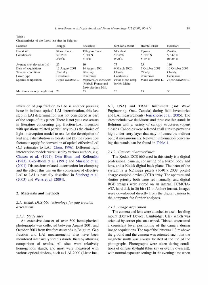
Table 1
Characteristics of the forest test sites in Belgium
Location Brugge Roeselare Sint-Joris-Weert Hechtel-Eksel Hoeilaart
Forest site Sterre forest Tillegem forest Meerdaal Pijnven Zonien
Coordinates 508550N 518100N 508480N 518100 N 508470 N
38080E 38110E 08200E 58190 E 048260 E
Average site elevation (m) 25 10 75 55 110
Date of acquisitions 13 August 2001 14 August 2001 6 March 2002 7 October 2002 10 October 2003
Weather conditions Blue sky Blue sky Cloudy Cloudy Cloudy
Cover type Deciduous Coniferous Coniferous Coniferous Deciduous
Species composition Fagus sylvatica L. Pseudotsuga menziesii
(Mirbel) Franco and
Larix decidua Mill.
Pinus nigra subsp.
laricio Maire
Pinus sylvestris L. Fagus sylvatica L.
Maximum canopy height (m) 20 35 20 25 30
inversion of gap fraction to LAI is another pressing
issue in indirect optical LAI determination, this last
step in LAI determination was not considered as part
of the scope of this paper. There is not yet a consensus
in literature concerning gap fraction-LAI inversion
with questions related particularly to (1) the choice of
light interception model to use for the description of
leaf angle distribution in forests and (2) the correction
factors to apply for conversion of optical effective LAI
(Le) estimates to LAI (Chen, 1996). Different light
interception models were used by various authors, e.g.
Chason et al. (1991), Oker-Blom and Kellomaki
(1983), Oker-Blom et al. (1991) and Mussche et al.
(2001). Discussions related to correction for clumping
and the effect this has on the conversion of effective
LAI to LAI is partially described in Stenberg et al.
(2003) and Weiss et al. (2004).
2. Materials and methods
2.1. Kodak DCS 660 technology for gap fraction
assessment
2.1.1. Study sites
An extensive dataset of over 300 hemispherical
photographs was collected between August 2001 and
October 2003 from five forests stands in Belgium. Gap
fraction and LAI measurements also have been
monitored intensively for this stands, thereby allowing
comparison of results. All sites were relatively
homogenous stands, and most were measured with
various optical devices, such as LAI-2000 (Licor Inc.,
NE, USA) and TRAC Instrument (3rd Wave
Engineering, Ont., Canada) during field inventories
and LAI measurements (Jonckheere et al., 2005). The
sites include two deciduous and three conifer stands in
Belgium with a variety of canopy structures (open/
closed). Canopies were selected at all sites to prevent a
high under-story layer that may influence the indirect
optical measurements. Relevant information concern-
ing the stands can be found in Table 1.
2.1.2. Camera characteristics
The Kodak DCS 660 used in this study is a digital
professional camera, consisting of a Nikon body and
lens, and a Kodak digital back plane. The heart of the
system is a 6.2 mega pixels (3040 � 2008 pixels)
charge-coupled-device (CCD) array. The aperture and
shutter priority both were set manually, and digital
RGB images were stored on an internal PCMCIA-
ATA hard disk in 36-bit (12-bit/color) format. Images
were downloaded directly from the digital camera to
the computer for further analyses.
2.1.3. Image acquisition
The camera and lens were attached to a self-leveling
mount (Delta-T Device, Cambridge, UK), which was
oriented by corner pins on a tripod. This set-up ensured
a consistent level positioning of the camera during
image acquisitions. The top of the lens was 1.3 m above
the ground and the camera was oriented such that the
magnetic north was always located at the top of the
photographs. Photographs were taken during condi-
tions of diffuse skylight (blue sky or evenly overcast),
with normal exposure settings in the evening time when
I. Jonckheere et al. / Agricultural and Forest Meteorology 132 (2005) 96–114100
the sun was under the skyline in order to minimize glare
from direct sunlight. Photographic images were
recorded using a Sigma 8 mm f/4 ‘fisheye’ lens (Sigma
Corporation, Tokyo, Japan) at the highest possible
resolution (3040 � 2008 pixels) with highest ISO
setting (ISO 200). Moreover, the focus ring was set
to infinity when using the fisheye lens, as depth of field
is practically infinite and focusing was not required
(Bockaert, 2004).
2.2. Data processing
2.2.1. Pre-processing of the images
The color hemispherical photographs were ana-
lysed using the ENVI (2004) image-processing
software package for Windows (RSI, Version 4.0,
CO, USA). As absorption of leafy material is maximal
and scattering of sky tends to be lowest in the blue
channel, the blue channel was chosen for subsequent
analysis based on previous research on low dynamic
range imagery. This highlighted maximal contrast
between leaf and sky and the compatibility with the
LAI-2000 that measures light intensities solely below
490 nm (Jacquemoud and Baret, 1990; Nackaerts
et al., 1999b). However, the smallest vegetation
elements might be invisible in the blue channel,
especially during blue sky conditions. This is due to
the limited quality of the hemispherical lens, which
suffers chromatic aberration, especially in the blue
part of the spectrum (Frazer et al., 2001). These
outcomes resulted in a trade-off effect between the two
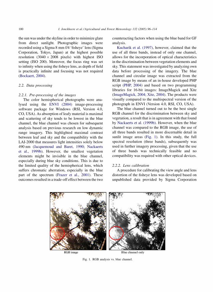
Fig. 1. RGB analysis v
counteracting factors when using the blue band for GF
analysis.
Kucharik et al. (1997), however, claimed that the
use of all three bands, instead of only one channel,
allows for the incorporation of optical characteristics
in the discrimination between vegetation elements and
sky. This statement was investigated by analyzing own
data before processing of the imagery. The blue
channel and circular image was extracted from the
RGB image by means of an in-house developed PHP
script (PHP, 2004) and based on two programming
libraries for 16-bit images: ImageMagick and Xite
(ImageMagick, 2004; Xite, 2004). The products were
visually compared to the multispectral version of the
photograph in ENVI (Version 4.0, RSI, CO, USA).
The blue channel turned out to be the best single
RGB channel for the discrimination between sky and
vegetation, a result that is in agreement with that found
by Nackaerts et al. (1999b). However, when the blue
channel was compared to the RGB image, the use of
all three bands resulted in more discernable detail in
sunlit image areas (Fig. 1). In this study, the full
spectral resolution (three bands), subsequently was
used in further imagery processing, given that the use
of three bands was technically feasible and no
compatibility was required with other optical devices.
2.2.2. Lens calibration
A procedure for calibrating the view angle and lens
distortion of the fisheye lens was developed based on
unpublished data provided by Sigma Corporation
s. blue channel.
I. Jonckheere et al. / Agricultural and Forest Meteorology 132 (2005) 96–114 101
(Tokyo, Japan). The data consisted of 23 specifications
with regard to the actual relationship between radial
distance r and zenith angle u. A lens correction function
was calculated based on calibration data to correct for
deviations from the equi-angular projection. This was
done in order to minimize aberrations due to the high
sensitivity of gap fraction analysis to angular distortion.
The relationship between radial distance r and zenith
angle uwas fitted by means of the statistical software of
Table Curve 2D (Version 4.0, Systat, London, UK) to a
polynomial expression of the form:
P0 ¼XN
i¼0
aiPi (1)
where i is the order of the term, N the order of the
polynomial expression, P0 the distance from the centre
of the image (in mm) and P is the zenith angle u in the
hemispherical object region. By changing the order of
the polynomial expression from unity to 20, the
change in the standard error estimate (SEE) with
the order N was analyzed (Zar, 1984). The expression
with minimum SEE was determined as the optimum
expression for calibrating the view angle and lens
distortion of the Sigma fisheye converter. The standard
error of polynomial correction expression decreased
significantly from the first- to third-order of term
from 0.25 to 0.0192. No more decrease in standard
error was shown after the third-order of term. Con-
sequently, the third-order polynomial expression was
determined as the optimum expression for calibrating
view angle and lens distortion because of the mini-
mum SEE (0.0192). The numerical coefficients were:
a0 = �0.0009, a1 = 0.1367, a2 = �0.0000154 and
a3 = �0.00000155, respectively. This polynomial
expression was used to correct the view angle and
lens distortions by substituting the radial distance at a
given point r and the radius of hemispherical photo-
graph R into the obtained polynomial expression in
ENVI.
Two more steps were required to derive gap fraction
from the digital RGB images: (1) the separation of pixel
intensities into sky and vegetation classes by thresh-
olding and (2) the calculation of gap fraction.
2.2.3. Thresholding
Thresholding is the simplest and most fundamental
segmentation method. In a gray level image, for
example, a gray value would be chosen such that
pixels with intensities below or equal to the treshold
would represent one class (e.g. feature), whereas those
above the threshold would represent the other (e.g.
background). This technique is used to transform a
color image into a black and white image. Thresh-
olding is an effective tool to separate vegetation from
sky, given that the gray levels of pixels representing
vegetation in hemispherical photographs are substan-
tially different from the gray levels of pixels belonging
to the sky background (Otsu, 1979; Sezgin and Sankur,
2004). The output of the thresholding operation is a
binary image whose foreground represents vegetation
and can be assigned a gray level of 0 (black), whereas
the background corresponds to the sky and can be
represented by a gray level of 65,535 in 16-bit (white).
Gap fraction can then easily be extracted as the ratio of
sky pixels to the total amount of pixels in the image,
given this binary image as input.
The shape of the gray scale histogram often
facilitates manual selection of the threshold value,
for example, with the mid-point or a valley between
two distinct peaks often used as threshold (Prewitt
and Mendelsohn, 1966). Unfortunately, this method
is undesirable for two reasons. First, the nature of the
image histogram may be uni- or multi-modal such
that the selection of the appropriate value is less
obvious. The threshold selection is unrepeatable
under these circumstances, due to the inherent
subjectivity in the decision-making process and
inter-operator variation. Secondly, manual thresh-
olding, apart from being extremely impractical for
image acquisitions dealing with large numbers of
images, can be complicated by various factors, such
as noise, ambient illumination and inadequate
contrast (Lievers and Pilkey, 2004).
The commonly used but subjective manual thresh-
olding will consequently be tested against automatic
methods for image binarization in this study.
For the manual thresholding, the image processing
software ENVI was used to allow the full dynamic
range (16 bits) of the images, thereby avoiding the
conversion of the data to a lower bit range and the
concomitant reduction in quality. Other commercial
available software packages for gap fraction and LAI
estimation could not be applied, as they are all limited
to 8-bit image processing. An experienced operator
selected for each image individually the best visual
I. Jonckheere et al. / Agricultural and Forest Meteorology 132 (2005) 96–114102
threshold in order to discriminate foliage from the sky
background. All pixels with brightness values higher
than the threshold are than classified as sky, whereas
all pixels lower than the threshold are foliage.
Concerning the automatic methods, however,
selecting an appropriate one can be a difficult task
since there are many automatic thresholding algo-
rithms published in literature. The caveat is that
different algorithms typically produce different
results, since they make different assumptions about
the image content. For instance, some require the two
classes to be dissimilar in size, while others model the
class distribution as normals, etc. (Rosin and
Ioannidis, 2003). The selection of segmentation
algorithms in this study was based on algorithms that
are widely known and straightforward to implement,
thereby ensuring that accurate coding was likely.
The selected automatic methods can be categorized
in six groups, according to the information they
require (see the overview by Sezgin and Sankur (2004)
for a description of the individual methods):
(1) H
istogram shape-based methods: this category ofmethods achieves thresholding based on the shape
properties of the histogram. Analysis is based on
the histogram of the luminance values in the
image (peaks, valleys, etc.). The tested methods in
this groups were the method of Rosenfeld, Sezan,
Olivo and Ramesh (e.g. Olivo, 1994).
(2) C
lustering-based thresholding methods: in thisclass of algorithms, the gray level data undergoes
a clustering analysis, with the number of clusters
set always to two. The gray levels are clustered in
two classes as background and foreground.
Examined methods were Ridler, Yanni, Otsu,
Lloyd, Kittler and Jawahar (e.g. Ridler and
Calvard, 1978).
(3) E
ntropy-based methods: this class exploits theentropy of the distribution of gray levels in an
image. The maximization of the entropy of the
thresholded image is interpreted as indicative of
maximum information transfer. Some algorithms
use the entropy of the foreground and background
regions, while others focus on the cross-entropy
between the original and binarized image, etc.
Methods of Kapur, Sahoo, Pun, Li, Brink and
Shanbag were investigated (e.g. Kapur et al.,
1985).
(4) O
bject attribute-based methods: these algorithmsselect the threshold value based on some attribute
quality or similarity measure between the original
image and the binarized version of the image.
These attributes can be, for example, edge
matching, connectivity, texture, shape compact-
ness, etc. The Tsai method, Hertz, OGorman,
Huang and Pikaz method were used (e.g. Tsai,
1985).
(5) S
patial methods: this class utilizes not only grayvalue distribution but also dependency of pixels in
a neighbourhood, for example, in the form of
correlation functions, 2D entropy, co-occurrence
probabilities and local linear dependence models.
High-order probability distribution and/or corre-
lation between pixels are then used for segmenta-
tion. The method of Pal, Abutaleb and Beghdadi
were tested (e.g. Abutaleb, 1989).
(6) L
ocal methods: in this class of algorithms, athreshold is calculated at each pixel, which
depends on some local statistics, such as range,
variance, etc. The threshold value is adapted to the
local image characteristics of the neighbourhood.
The method of Niblack, Sauvola, White, Bernsen,
Palumbo, Kamel, and Yanowitz was tested as
representative of this group (e.g. Niblack, 1986).
The different categories tested in this study and
their main characteristics and threshold determination
are shown in Table 2. Further details regarding each
algorithm are provided in the respective references
and in the overview of Sezgin and Sankur (2004).
Image segmentation, and thresholding in particular,
is a body of research that is important in fields as
diverse as document analysis, medical imaging and
computer vision. While many different thresholding
algorithms have been proposed, the appropriate
selection is application-dependent. The automatic
methods tested in this study consequently are widely
used in the field of microscopy and medicine, but only
few of them were used and/or investigated to optimise
thresholding in hemispherical canopy photography.
For example, Weiss (2003) used the convex-hull
thresholding method (as histogram shape-base
thresholding) in EYE-CAN Version 1.4 and Nackaerts
et al. (1999a) used the Cluster–Otsu method combined
with the local Niblack method to correct for light
errors in 24-bit photographs. In most studies and
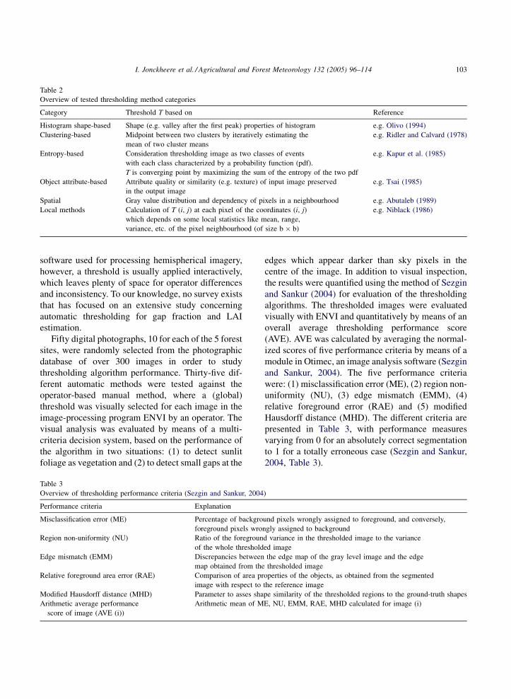
I. Jonckheere et al. / Agricultural and Forest Meteorology 132 (2005) 96–114 103
Table 2
Overview of tested thresholding method categories
Category Threshold T based on Reference
Histogram shape-based Shape (e.g. valley after the first peak) properties of histogram e.g. Olivo (1994)
Clustering-based Midpoint between two clusters by iteratively estimating the
mean of two cluster means
e.g. Ridler and Calvard (1978)
Entropy-based Consideration thresholding image as two classes of events
with each class characterized by a probability function (pdf).
T is converging point by maximizing the sum of the entropy of the two pdf
e.g. Kapur et al. (1985)
Object attribute-based Attribute quality or similarity (e.g. texture) of input image preserved
in the output image
e.g. Tsai (1985)
Spatial Gray value distribution and dependency of pixels in a neighbourhood e.g. Abutaleb (1989)
Local methods Calculation of T (i, j) at each pixel of the coordinates (i, j)
which depends on some local statistics like mean, range,
variance, etc. of the pixel neighbourhood (of size b � b)
e.g. Niblack (1986)
software used for processing hemispherical imagery,
however, a threshold is usually applied interactively,
which leaves plenty of space for operator differences
and inconsistency. To our knowledge, no survey exists
that has focused on an extensive study concerning
automatic thresholding for gap fraction and LAI
estimation.
Fifty digital photographs, 10 for each of the 5 forest
sites, were randomly selected from the photographic
database of over 300 images in order to study
thresholding algorithm performance. Thirty-five dif-
ferent automatic methods were tested against the
operator-based manual method, where a (global)
threshold was visually selected for each image in the
image-processing program ENVI by an operator. The
visual analysis was evaluated by means of a multi-
criteria decision system, based on the performance of
the algorithm in two situations: (1) to detect sunlit
foliage as vegetation and (2) to detect small gaps at the
Table 3
Overview of thresholding performance criteria (Sezgin and Sankur, 2004
Performance criteria Explanation
Misclassification error (ME) Percentage of backgro
foreground pixels wro
Region non-uniformity (NU) Ratio of the foregroun
of the whole threshold
Edge mismatch (EMM) Discrepancies between
map obtained from the
Relative foreground area error (RAE) Comparison of area pr
image with respect to
Modified Hausdorff distance (MHD) Parameter to asses sha
Arithmetic average performance
score of image (AVE (i))
Arithmetic mean of M
edges which appear darker than sky pixels in the
centre of the image. In addition to visual inspection,
the results were quantified using the method of Sezgin
and Sankur (2004) for evaluation of the thresholding
algorithms. The thresholded images were evaluated
visually with ENVI and quantitatively by means of an
overall average thresholding performance score
(AVE). AVE was calculated by averaging the normal-
ized scores of five performance criteria by means of a
module in Otimec, an image analysis software (Sezgin
and Sankur, 2004). The five performance criteria
were: (1) misclassification error (ME), (2) region non-
uniformity (NU), (3) edge mismatch (EMM), (4)
relative foreground error (RAE) and (5) modified
Hausdorff distance (MHD). The different criteria are
presented in Table 3, with performance measures
varying from 0 for an absolutely correct segmentation
to 1 for a totally erroneous case (Sezgin and Sankur,
2004, Table 3).
)
und pixels wrongly assigned to foreground, and conversely,
ngly assigned to background
d variance in the thresholded image to the variance
ed image
the edge map of the gray level image and the edge
thresholded image
operties of the objects, as obtained from the segmented
the reference image
pe similarity of the thresholded regions to the ground-truth shapes
E, NU, EMM, RAE, MHD calculated for image (i)

I. Jonckheere et al. / Agricultural and Forest Meteorology 132 (2005) 96–114104
A single thresholding method that results in perfect
agreement with the standard reference image is
unlikely, given the methods of thresholding described
above. Nevertheless, there will always be a thresh-
olding method that will yield the closest possible
agreement results, being most robust in terms of
both visual and quantitative analysis. We refer to
this as the ‘‘optimal’’ thresholding method. This
technique will be further evaluated in the sensitivity
analysis.
2.2.4. Gap fraction estimation
The last step in the interpretation of the classified
hemispherical photographs in terms of gap fraction is
the calculation of the gap fraction from the binary
black-and-white images. Gap fraction, defined as the
fraction of open sky not obstructed by canopy
elements, can easily be calculated for different zenith
and azimuth angles. This is done by counting the
amount of sky pixels and vegetation pixels by means
of the following formula:
Tðu;aÞ ¼ Ps
Ps þ Pns
(2)
where T(u, a) is the gap fraction for a range of zenith
angles with mean angle u and angular resolution a; Ps
is the number of pixels classified as ‘‘sky pixels’’ in a
region centred at (u, a) and Pns is the number of
vegetation pixels within a region centred at (u, a).
GF was computed after calibrating the view angle and
lens distortions of the Sigma fisheye lens. All photo-
graph processing were fully automatized by means of
an in-house developed IDL (2004) script to extract gap
fraction (IDL, Version 6.1, RSI, USA), resulting in no
interference by an operator. The comparison between
the different digital photographs in the sensitivity
analysis, where the effect of threshold and operator
bias was examined, was done at the resulting gap
fraction level to gain a good understanding of the
influencing factors.
3. Results
In this section we present the results obtained by
following the testing protocol of both visual inspection
and the quantitative performance analysis.
3.1. Visual analysis
The results of the visual analysis of 50 photographs
thresholded by the different thresholding algorithms are
listed in Table 4. Apart from algorithm performance in
the centre of the image (to detect sunlit foliage as
vegetation) and at the edges (to pick up small gaps
which appear darker than the sky pixels in the centre of
the image), the overall visual appearance (artificial
patterns) of the image also was investigated (Table 4).
Worst and best case images, based on visual
inspection for each of the six investigated thresholding
method categories, are given in Fig. 3. These are
shown along with the reference ground-truth images
and the manually thresholded image.
At first glance, the results in Table 4 showed that
most of the algorithms performed better under bright
conditions than in dark regions. The histogram shape-
based and local thresholding algorithms generally were
too sensitive to overall image differences in gray levels
in the hemispherical canopy photographs. Fig. 3j
illustrates this problem. Small differences in gray levels
between stems and background vegetation, for exam-
ple, caused the Sezan algorithm to select a threshold
value in-between, thereby classifying slightly brighter
background vegetation as sky. Fig. 3a and b illustrate
the local white and Niblack methods, which were even
more sensitive and resulted in extremely noisy images.
The method of Rosenfeld, also a local thresholding
method was not sensitive enough, and many vegetation
pixels were lost by this technique (Fig. 2c). It shows
that at the edge of the image and on areas with a
closer canopy, small gaps in the canopy were strongly
exaggerated. Some of the entropy, attribute-based and
local algorithms (e.g. Pikaz, Bernsen) performed well
in the centre of the image, but tended to classify too
many pixels as vegetation at the edges, which yielded
too dark results (Fig. 3c and d).
Other methods, for example, shape Olivo and
entropy Shanbag, were not sensitive enough and many
vegetation pixels were lost by these techniques
(Fig. 3e and f). Some methods exhibited artifacts
after thresholding, for example, the object attribute-
based OGorman method and the local Yasuda method,
which resulted in angular and abrupt edges (Fig. 3g
and h). Algorithms that performed best in visual terms
were the clustering method of Ridler, the attribute-
based method of Hertz, and the spatial method of
I. Jonckheere et al. / Agricultural and Forest Meteorology 132 (2005) 96–114 105
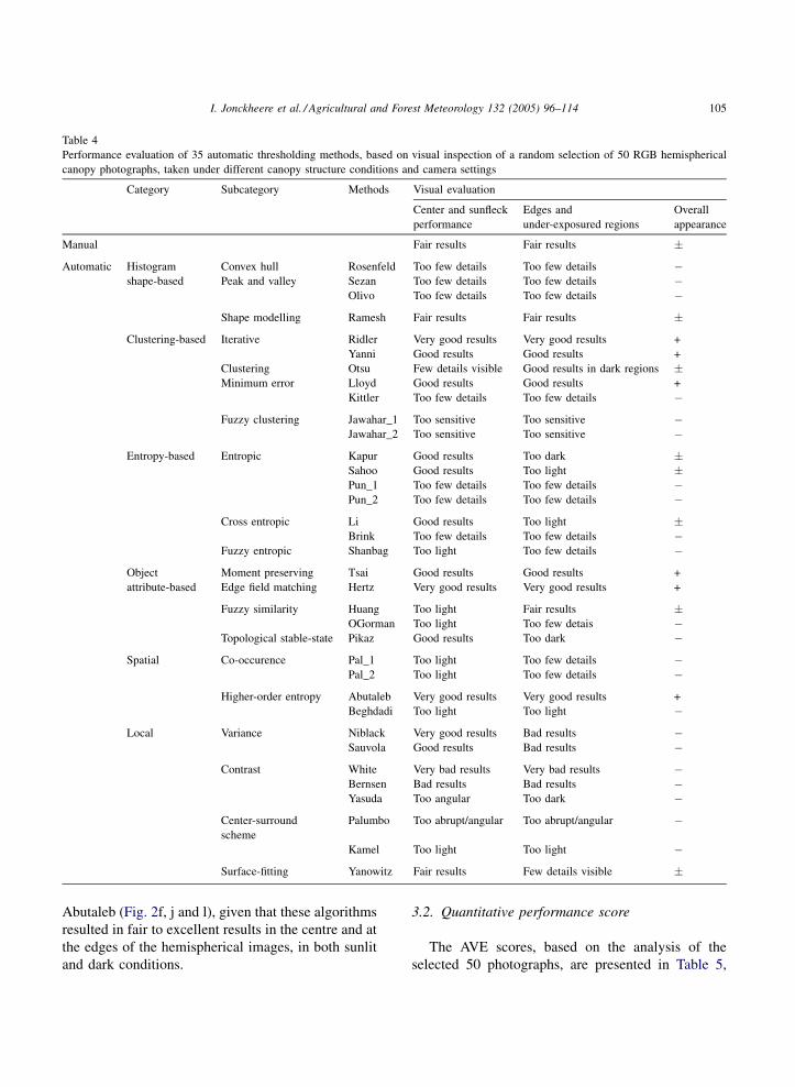
Table 4
Performance evaluation of 35 automatic thresholding methods, based on visual inspection of a random selection of 50 RGB hemispherical
canopy photographs, taken under different canopy structure conditions and camera settings
Category Subcategory Methods Visual evaluation
Center and sunfleck
performance
Edges and
under-exposured regions
Overall
appearance
Manual Fair results Fair results �
Automatic Histogram
shape-based
Convex hull Rosenfeld Too few details Too few details �Peak and valley Sezan Too few details Too few details �
Olivo Too few details Too few details �
Shape modelling Ramesh Fair results Fair results �
Clustering-based Iterative Ridler Very good results Very good results +
Yanni Good results Good results +
Clustering Otsu Few details visible Good results in dark regions �Minimum error Lloyd Good results Good results +
Kittler Too few details Too few details �
Fuzzy clustering Jawahar_1 Too sensitive Too sensitive �Jawahar_2 Too sensitive Too sensitive �
Entropy-based Entropic Kapur Good results Too dark �Sahoo Good results Too light �Pun_1 Too few details Too few details �Pun_2 Too few details Too few details �
Cross entropic Li Good results Too light �Brink Too few details Too few details �
Fuzzy entropic Shanbag Too light Too few details �
Object
attribute-based
Moment preserving Tsai Good results Good results +
Edge field matching Hertz Very good results Very good results +
Fuzzy similarity Huang Too light Fair results �OGorman Too light Too few detais �
Topological stable-state Pikaz Good results Too dark �
Spatial Co-occurence Pal_1 Too light Too few details �Pal_2 Too light Too few details �
Higher-order entropy Abutaleb Very good results Very good results +
Beghdadi Too light Too light �
Local Variance Niblack Very good results Bad results �Sauvola Good results Bad results �
Contrast White Very bad results Very bad results �Bernsen Bad results Bad results �Yasuda Too angular Too dark �
Center-surround
scheme
Palumbo Too abrupt/angular Too abrupt/angular �
Kamel Too light Too light �
Surface-fitting Yanowitz Fair results Few details visible �
Abutaleb (Fig. 2f, j and l), given that these algorithms
resulted in fair to excellent results in the centre and at
the edges of the hemispherical images, in both sunlit
and dark conditions.
3.2. Quantitative performance score
The AVE scores, based on the analysis of the
selected 50 photographs, are presented in Table 5,
I. Jonckheere et al. / Agricultural and Forest Meteorology 132 (2005) 96–114106
grouped per thresholding method category. Since AVE
is an error score ranging from 0 to 1, the lower AVE
(near 0), the better the performance of the algorithm,
whereas the higher AVE (towards 1), the worse the
performance.
According to the quantitative AVE scores, the 10
best methods were from the clustering, entropy, shape
Fig. 2. Results of the worst and best thresholding algorithms for the six te
reference ground-truth hemispherical canopy image and manually thresho
and attribute categories, which indicated the quanti-
tative potential of these categories to binarization of
hemispherical canopy images. However, given that the
AVE is an average score based on five performance
criteria, caution is somehow required since a method
might have insufficient visual results and nevertheless
a low AVE score (and vice versa). Fig. 3i illustrates
sted algorithm categories base on visual inspection, compared to the
lded image.
I. Jonckheere et al. / Agricultural and Forest Meteorology 132 (2005) 96–114 107
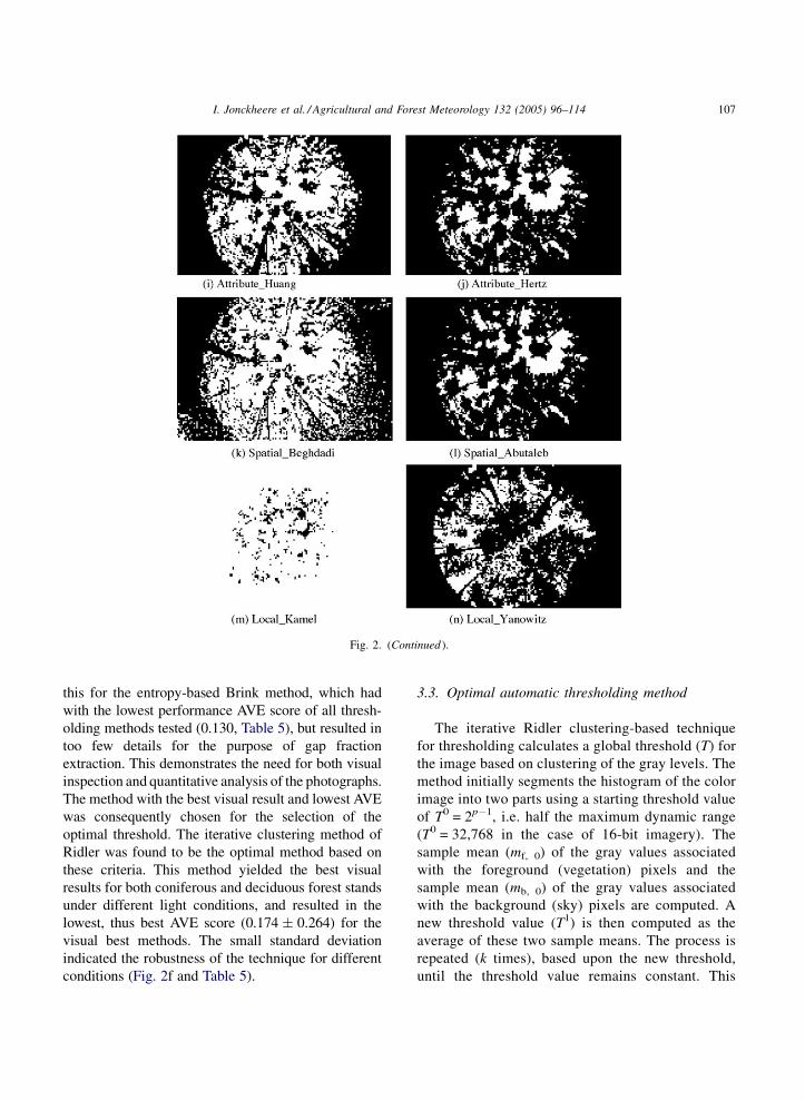
Fig. 2. (Continued ).
this for the entropy-based Brink method, which had
with the lowest performance AVE score of all thresh-
olding methods tested (0.130, Table 5), but resulted in
too few details for the purpose of gap fraction
extraction. This demonstrates the need for both visual
inspection and quantitative analysis of the photographs.
The method with the best visual result and lowest AVE
was consequently chosen for the selection of the
optimal threshold. The iterative clustering method of
Ridler was found to be the optimal method based on
these criteria. This method yielded the best visual
results for both coniferous and deciduous forest stands
under different light conditions, and resulted in the
lowest, thus best AVE score (0.174 � 0.264) for the
visual best methods. The small standard deviation
indicated the robustness of the technique for different
conditions (Fig. 2f and Table 5).
3.3. Optimal automatic thresholding method
The iterative Ridler clustering-based technique
for thresholding calculates a global threshold (T) for
the image based on clustering of the gray levels. The
method initially segments the histogram of the color
image into two parts using a starting threshold value
of T0 = 2p�1, i.e. half the maximum dynamic range
(T0 = 32,768 in the case of 16-bit imagery). The
sample mean (mf, 0) of the gray values associated
with the foreground (vegetation) pixels and the
sample mean (mb, 0) of the gray values associated
with the background (sky) pixels are computed. A
new threshold value (T1) is then computed as the
average of these two sample means. The process is
repeated (k times), based upon the new threshold,
until the threshold value remains constant. This
I. Jonckheere et al. / Agricultural and Forest Meteorology 132 (2005) 96–114108
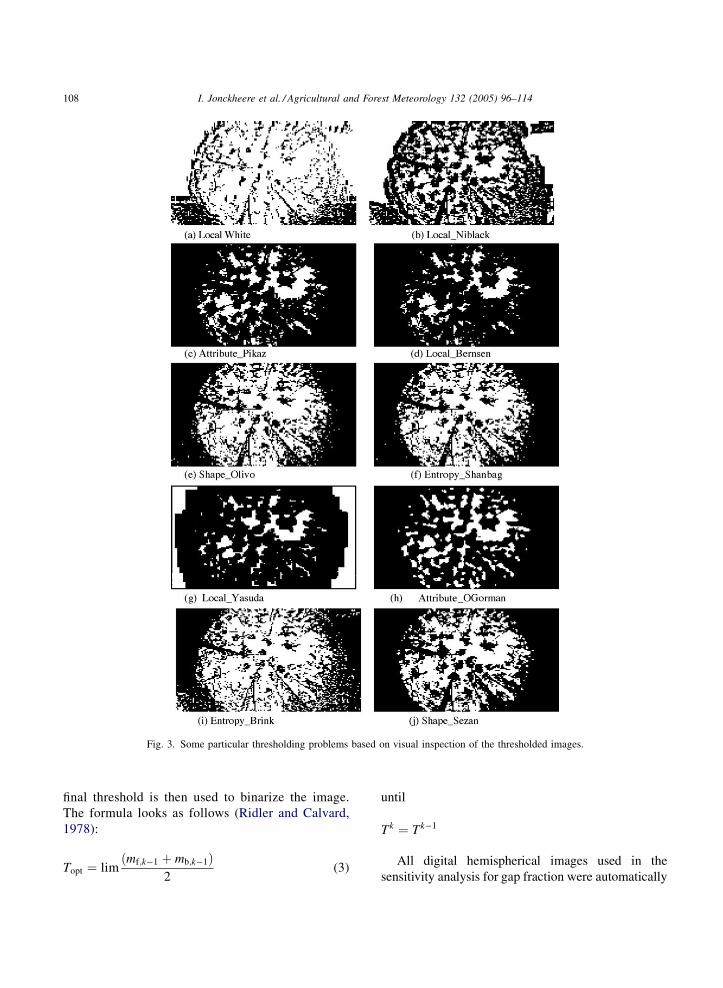
Fig. 3. Some particular thresholding problems based on visual inspection of the thresholded images.
final threshold is then used to binarize the image.
The formula looks as follows (Ridler and Calvard,
1978):
Topt ¼ limðmf;k�1 þ mb;k�1Þ
2(3)
until
Tk ¼ Tk�1
All digital hemispherical images used in the
sensitivity analysis for gap fraction were automatically
I. Jonckheere et al. / Agricultural and Forest Meteorology 132 (2005) 96–114 109
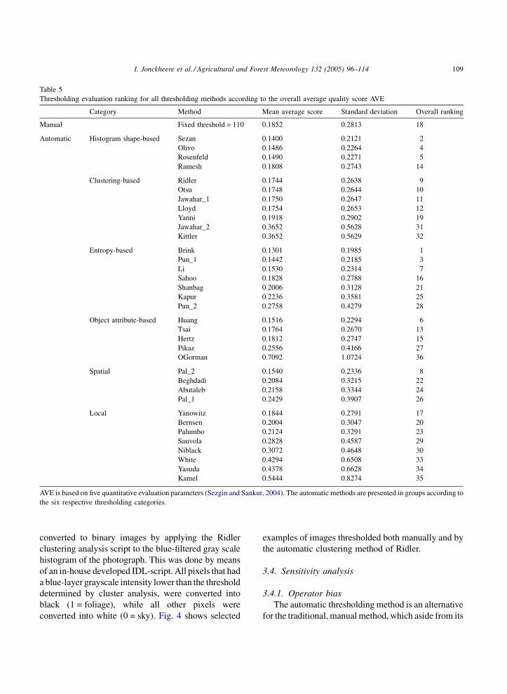
Table 5
Thresholding evaluation ranking for all thresholding methods according to the overall average quality score AVE
Category Method Mean average score Standard deviation Overall ranking
Manual Fixed threshold = 110 0.1852 0.2813 18
Automatic Histogram shape-based Sezan 0.1400 0.2121 2
Olivo 0.1486 0.2264 4
Rosenfeld 0.1490 0.2271 5
Ramesh 0.1808 0.2743 14
Clustering-based Ridler 0.1744 0.2638 9
Otsu 0.1748 0.2644 10
Jawahar_1 0.1750 0.2647 11
Lloyd 0.1754 0.2653 12
Yanni 0.1918 0.2902 19
Jawahar_2 0.3652 0.5628 31
Kittler 0.3652 0.5629 32
Entropy-based Brink 0.1301 0.1985 1
Pun_1 0.1442 0.2185 3
Li 0.1530 0.2314 7
Sahoo 0.1828 0.2788 16
Shanbag 0.2006 0.3128 21
Kapur 0.2236 0.3581 25
Pun_2 0.2758 0.4279 28
Object attribute-based Huang 0.1516 0.2294 6
Tsai 0.1764 0.2670 13
Hertz 0.1812 0.2747 15
Pikaz 0.2556 0.4166 27
OGorman 0.7092 1.0724 36
Spatial Pal_2 0.1540 0.2336 8
Beghdadi 0.2084 0.3215 22
Abutaleb 0.2158 0.3344 24
Pal_1 0.2429 0.3907 26
Local Yanowitz 0.1844 0.2791 17
Bernsen 0.2004 0.3047 20
Palumbo 0.2124 0.3291 23
Sauvola 0.2828 0.4587 29
Niblack 0.3072 0.4648 30
White 0.4294 0.6508 33
Yasuda 0.4378 0.6628 34
Kamel 0.5444 0.8274 35
AVE is based on five quantitative evaluation parameters (Sezgin and Sankur, 2004). The automatic methods are presented in groups according to
the six respective thresholding categories.
converted to binary images by applying the Ridler
clustering analysis script to the blue-filtered gray scale
histogram of the photograph. This was done by means
of an in-house developed IDL-script. All pixels that had
a blue-layer grayscale intensity lower than the threshold
determined by cluster analysis, were converted into
black (1 = foliage), while all other pixels were
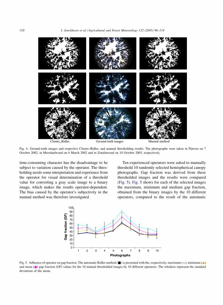
converted into white (0 = sky). Fig. 4 shows selected
examples of images thresholded both manually and by
the automatic clustering method of Ridler.
3.4. Sensitivity analysis
3.4.1. Operator bias
The automatic thresholding method is an alternative
for the traditional, manual method, which aside from its
I. Jonckheere et al. / Agricultural and Forest Meteorology 132 (2005) 96–114110
Fig. 4. Ground-truth images and respective Cluster–Ridler, and manual thresholding results. The photographs were taken in Pijnven on 7
October 2002, in Meerdaalwoud on 6 March 2002 and in Zonienwoud on 10 October 2003, respectively.
time-consuming character has the disadvantage to be
subject to variation caused by the operator. The thres-
holding needs some interpretation and experience from
the operator for visual determination of a threshold
value for converting a gray scale image to a binary
image, which makes the results operator-dependent.
The bias caused by the operator’s subjectivity in the
manual method was therefore investigated.
Fig. 5. Influence of operator on gap fraction. The automatic Ridler method
and mean ( ) gap fraction (GF) values for the 10 manual thresholded im
deviations of the mean.
Ten experienced operators were asked to manually
threshold 10 randomly selected hemispherical canopy
photographs. Gap fraction was derived from these
thresholded images and the results were compared
(Fig. 5). Fig. 5 shows for each of the selected images
the maximum, minimum and medium gap fraction,
obtained from the binary images by the 10 different
operators, compared to the result of the automatic
(&) is presented with the, respectively, maximum (�), minimum ( )
ages by 10 different operators. The whiskers represent the standard
I. Jonckheere et al. / Agricultural and Forest Meteorology 132 (2005) 96–114 111
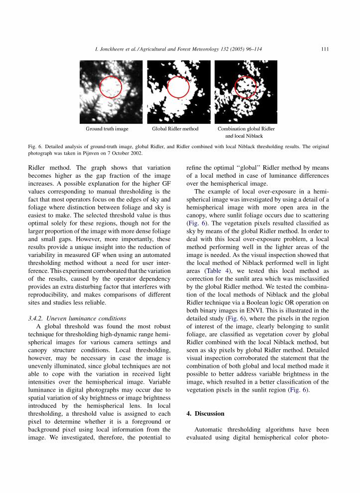
Fig. 6. Detailed analysis of ground-truth image, global Ridler, and Ridler combined with local Niblack thresholding results. The original
photograph was taken in Pijnven on 7 October 2002.
Ridler method. The graph shows that variation
becomes higher as the gap fraction of the image
increases. A possible explanation for the higher GF
values corresponding to manual thresholding is the
fact that most operators focus on the edges of sky and
foliage where distinction between foliage and sky is
easiest to make. The selected threshold value is thus
optimal solely for these regions, though not for the
larger proportion of the image with more dense foliage
and small gaps. However, more importantly, these
results provide a unique insight into the reduction of
variability in measured GF when using an automated
thresholding method without a need for user inter-
ference. This experiment corroborated that the variation
of the results, caused by the operator dependency
provides an extra disturbing factor that interferes with
reproducibility, and makes comparisons of different
sites and studies less reliable.
3.4.2. Uneven luminance conditions
A global threshold was found the most robust
technique for thresholding high-dynamic range hemi-
spherical images for various camera settings and
canopy structure conditions. Local thresholding,
however, may be necessary in case the image is
unevenly illuminated, since global techniques are not
able to cope with the variation in received light
intensities over the hemispherical image. Variable
luminance in digital photographs may occur due to
spatial variation of sky brightness or image brightness
introduced by the hemispherical lens. In local
thresholding, a threshold value is assigned to each
pixel to determine whether it is a foreground or
background pixel using local information from the
image. We investigated, therefore, the potential to
refine the optimal ‘‘global’’ Ridler method by means
of a local method in case of luminance differences
over the hemispherical image.
The example of local over-exposure in a hemi-
spherical image was investigated by using a detail of a
hemispherical image with more open area in the
canopy, where sunlit foliage occurs due to scattering
(Fig. 6). The vegetation pixels resulted classified as
sky by means of the global Ridler method. In order to
deal with this local over-exposure problem, a local
method performing well in the lighter areas of the
image is needed. As the visual inspection showed that
the local method of Niblack performed well in light
areas (Table 4), we tested this local method as
correction for the sunlit area which was misclassified
by the global Ridler method. We tested the combina-
tion of the local methods of Niblack and the global
Ridler technique via a Boolean logic OR operation on
both binary images in ENVI. This is illustrated in the
detailed study (Fig. 6), where the pixels in the region
of interest of the image, clearly belonging to sunlit
foliage, are classified as vegetation cover by global
Ridler combined with the local Niblack method, but
seen as sky pixels by global Ridler method. Detailed
visual inspection corroborated the statement that the
combination of both global and local method made it
possible to better address variable brightness in the
image, which resulted in a better classification of the
vegetation pixels in the sunlit region (Fig. 6).
4. Discussion
Automatic thresholding algorithms have been
evaluated using digital hemispherical color photo-
I. Jonckheere et al. / Agricultural and Forest Meteorology 132 (2005) 96–114112
graphs of forest canopies. The results of this thresh-
olding step are very important as it has significant
influence on the subsequent gap fraction determina-
tion. Under-thresholding is undesirable as it can lead
to the loss of foliage, particularly where sunlit foliage
is classified as sky. Conversely, the dangers of over-
thresholding can be much more subtle and might even
extend beyond over-estimation of the gap fraction.
This has off course a major impact on the estimated
gap fraction out of the hemispherical images.
The visual inspection of the photographs by means
of multi-criteria analysis resulted in the identification
of three well-performing algorithms: the Cluster–
Ridler method, the object-attribute based method of
Hertz, and the spatially based Abutaleb method.
The good performance of the Ridler method is in
agreement with Lievers and Pilkey (2004), who
studied segmentation of automotive aluminium sheet
alloys. However, no absolute comparison is possible,
since the performance of thresholding algorithms are
application-based and there are no known studies
concerning the application of this algorithm in a
forestry context.
The quantitative analysis resulted in a top 10
ranking of methods of the groups of cluster, shape-
based, object attribute-based and entropy, which is in
agreement with Sezgin and Sankur (2004). The
authors ranked the categories of clustering and entropy
highest, and thus most plausible for thresholding of
non-destructive images. The clustering method of
Ridler was considered the ‘‘optimal’’ automatic
thresholding method for the binarization of hemi-
spherical photographs, based on the combination of
visual analysis and the performance analysis of the
AVE values. The algorithm is able to produce accurate
silhouettes for the extraction of gap fraction from the
blue-layer images of tree canopies, and has been found
to be the most robust automatic thresholding
technique for the different stand types (deciduous/
coniferous and open/closed). This technique, which
gave satisfactory results at image edges and in the
center, for both dark and sunlit conditions, performed
better than the other algorithms in terms of robustness
under varying conditions. The clustering method of
Ridler also achieved the best overall calculated
performance AVE value. Some methods did perform
well under specific sky conditions (sunlit or dark), but
yielded unacceptable results under the opposite
condition. The clustering Otsu and local Niblack
method are examples of this, and performed well in,
respectively, dark/sunlit regions, but were unable to
distinguish foliage from sky in overly light/dark
conditions. Local thresholding techniques were found
to be inappropriate for application at photo-level.
This was due to too little detail visible in the image
centre and at the edges, which caused a substantial
over-estimation of the gap fraction and consequently
a significant under-estimation of LAI. This poor
performance was attributed to the high level of
complexity of such photographs.
The automatic methods also were very time-
efficient, whereas interactive thresholding was very
time-consuming. This suggests that, apart from the
potential to provide an objective measure for canopy
structure and light measurement, automatic thresh-
olding allows considerably faster image processing.
In case of variable brightness over the hemisphe-
rical image, the combination of the local Niblack
method with the Ridler method gave a superior
performance over the existing optimal global Ridler
thresholding technique, as the local method was able
to cope with local over-exposure. More information
should be used to assist the thresholding, and thus
greater accuracy and more consistent performance is
required in order to correct for these technical
problems.
5. Concluding remarks
The global clustering method of Ridler was found
to be the optimal and most robust automatic thresh-
olding method for a wide range of light and canopy
structure conditions. This automatic method was most
robust in terms of both visual and quantitative analyses
and provides a useful baseline against which more
advanced algorithms can be evaluated. It therefore
offers an alternative towards a fast, reliable and
objective use of hemispherical photographs for gap
fraction and LAI estimation in forest stands. A high
level of accuracy and reproducibility is maintained,
since the impact of the operator on the thresholding of
high-dynamic range images revealed a considerable
variation in gap fraction results. This variation does
not occur when using automatic methods, which
provides the advantage of repeatability and reliability
I. Jonckheere et al. / Agricultural and Forest Meteorology 132 (2005) 96–114 113
to compare different studies and sites in a more
objective manner.
However, attention must be paid to the possible
potential of fine-tuning of local thresholding methods
to better address particular photographic limitations
(e.g. over-exposure in a certain image region). The
main scope of this study has been to find an alternative
to the subjective manual thresholding method, and
therefore enables further research to be done in
order to address particular photographic problems.
The use of new or more complex algorithms (tri- or
multi-level thresholding) also might be tested,
together with an investigation into the influence of
image smoothing for noise elimination. Since ‘‘real’’
gap fraction cannot be explicitly measured, this
evaluation has only a relative and not an absolute
value. This issue can be addressed in the future by
simulating virtual forest stands with known gap
fractions, from which the optimal selected method
can be validated by means of virtual hemispherical
photographs.
Acknowledgements
We would like to thank Sigma Corporation (Tokyo,
Japan) for providing us with data on the lens distortion
for the Sigma 8 mm f/4 ‘fisheye’ lens, used in the
study. We would like to acknowledge the useful
comments and criticisms about thresholding provided
by Dr. Mehmet Sezgin (Tubytak Marmara Research
Centre, Gebze, Kocaeli, Turkey). The valuable editing
by Dr. Jan Van Aardt also is deeply appreciated.
Funding support for this research has been provided by
FWO Flanders (Project no. G.0085.01).
References
Abutaleb, A.S., 1989. Automatic thresholding of gray-level pictures
using two-dimensional entropy. Comput. Vision Graph. Image
Proc. 47, 22–32.
Ackerly, D.D., Bazzaz, F.A., 1995. Seedling crown orientation and
interception of diffuse radiation in tropical forest gaps. Ecology
76, 1134–1146.
Battaglia, M.A., Mou, P., Palik, B., Mitchell, R.J., 2002. The effect
of spatially variable overstory on the understory light environ-
ment of an open-canopied longleaf pine forest. Can. J. Forest
Res. 32, 1984–1991.
Blennow, K., 1995. Sky view factors from high-resolution scanned
fish-eye lens photographic negatives. J. Atmos. Ocean. Tech. 12,
1357–1362.
Bockaert, V., 2004. The 123 of Digital Imaging Interactive Learning
Suite, Version 3.0, p. 2780 (CD).
Chason, J.W., Baldocchi, D.D., Huston, M.A., 1991. A comparison
of direct and indirect methods for estimating forest canopy leaf-
area. Agric. Forest Meteorol. 57, 107–128.
Chen, J.M., 1996. Optically-based methods for measuring seasonal
variation of leaf area index in boreal conifer stands. Agric. Forest
Meteorol. 80, 135–163.
Chen, J.M., Black, T.A., Adams, R.S., 1991. Evaluation of hemi-
spherical photography for determining plant area index and
geometry of a forest stand. Agric. Forest Meteorol. 56, 129–143.
Englund, S.R., O’Brien, J.J., Clark, D.B., 2000. Evaluation of digital
and film hemispherical photography for predicting understorey
light in a Bornean tropical rain forest. Agric. Forest Meteorol.
97, 129–139.
ENVI, 2004. Information available from, http://www.rsinc.com/
envi/.
Fernandes, R., Miller, J.R., Chen, J.M., Rubinstein, I.G., 2003.
Evaluating image-based estimates of leaf area index in boreal
conifer stands over a range of scales using high-resolution CASI
imagery. Remote Sens. Environ. 89, 200–216.
Fraser, C.S., 1997. Digital camera self-calibration. Photogramm.
Eng. Remote Sens. 52, 149–159.
Frazer, G.W., Trofymow, J.A., Lertzman, K.P., 1997. A method for
estimating canopy openness, effective leaf area index, and photo
synthetically active photon flux density using hemispherical
photography and computerized image analysis techniques.
K.P. Nat. Res. Canada, Can. For. Serv. Pacific For. Cent. Inf.
Re BC-X-373, 75 p.
Frazer, G.W., Fournier, R.A., Trofymow, J.A., Hall, R.J.A., 2001.
Comparison of digital and film fisheye photography for analysis
of forest canopy structure and gap light transmission. Agric.
Forest Meteorol. 109, 249–263.
Hale, S.E., Edwards, C., 2002. Comparison of film and digital
hemispherical photography across a wide range of canopy
densities. Agric. Forest Meteorol. 112, 51–56.
Herbert, T.J., 1986. Calibration of fisheye lenses by inversion of area
projections. Appl. Opt. 25, 1875–1876.
Hinz, A., Dorstel, C., Heier, H., 2001. DMC2001-The Z/I imaging
digital camera system. In: Proceedings of ASPRS Conference:
Gateway to the New Millennium, 23–27 April, St. Louis,
Missouri, USA, p. 3.
IDL, 2004. Information available from, http://www.rsinc.com/idl/.
ImageMagick, 2004. Information available from, www.imagema-
gick.org.
Jacquemoud, S., Baret, F., 1990. Prospect—a model of leaf optical-
properties spectra. Remote Sens. Environ. 34, 75–91.
Jonckheere, I., Fleck, S., Nackaerts, K., Muys, B., Coppin, P., Weiss,
M., Baret, F., 2004. Review of methods for in situ leaf area index
determination. Part I. theories, sensors and hemispherical photo-
graphy. Agric. Forest Meteorol. 121, 19–35.
Jonckheere, I., Muys, B., Coppin, P., 2005. Allometry and evaluation
of in-situ optical LAI determination: a case-study in Belgium.
Tree Physiol. 25 (6), 723–732.
I. Jonckheere et al. / Agricultural and Forest Meteorology 132 (2005) 96–114114
Kapur, J., Sahoo, P., Wong, A., 1985. A new method for gray-level
picture thresholding using the netropy of the histogram. Comput.
Vision Graph. Image Proc. 29, 273–285.
Koller, D., Weber, J., Malik, J., 1994. Robust multiple car tracking
with occlusion reasoning. In: European Conference of Computer
Vision. pp. 189–196.
Kucharik, C.J., Norman, J.M., Murdock, L.M., Gower, S.T., 1997.
Characterizing canopy non-randomness with a multiband vege-
tation imager (MVI). J. Geophys. Res. 102, 29455–29473.
Lievers, W.B., Pilkey, A.K., 2004. An evaluation of global thresh-
olding techniques for the automatic image segmentation of
automotive aluminium sheet alloys. Mater. Sci. Eng. 381,
134–142.
Mussche, S., Samson, R., Nachtergale, L., De Schrijver, A., Lemeur,
R., Lust, N.A., 2001. Comparison of optical and direct methods
for monitoring the seasonal dynamics of leaf area index in
deciduous forests. Silva Fenn. 35, 373–384.
Nackaerts, K., Sterckx, S., Coppin, P., 1999a. Fractal dimension as
correction factor for stand-level indirect leaf area index
measurements. In: Proceedings of EOS/SPIE Symposium on
Remote Sensing: Remote Sensing for Agriculture, Ecosystems,
and Hydrology III, 20–24 September, Florence, Italy, pp. 80–
89.
Nackaerts, K., Wagendorp, T., Coppin, P., Muys, B., Gombeer, R.,
1999b. A correction of indirect LAI measurements for a non-
random distribution of needles on shoots. In: Proceedings of
ISSSR: Systems and Sensors for the New Millennium, October
31–4 November, Las Vegas, Nevada, USA, pp. 413–424.
Niblack, W., 1986. An Introduction to Image Processing. Prentice-
Hall, Englewood Cliffs, NJ, pp. 115–116.
Oker-Blom, P., Kellomaki, S., 1983. Effect of grouping of foliage on
the within-stand and within-crown light regime: comparison of
random and grouping canopy models. Agric. Forest Meteorol.
28, 143–155.
Oker-Blom, P., Kaufmann, M.R., Ryan, M.G., 1991. Performance of
a canopy light interception model for conifer shoots, trees and
stands. Tree Physiol. 9, 227–243.
Olivo, J.C., 1994. Automatic threshold selection using the wavelet
transform. Graph. Models Image Process 56, 205–218.
Otsu, N., 1979. A threshold selection method from gray level
histograms. IEEE Trans. Syst. Man. Cybern. SMC 9, 62–66.
Ozanne, C.M.P., Anhuf, D., Boulter, S.L., Keller, M., Kitching, R.L.,
Korner, C., Meinzer, F.C., Mitchell, A.W., Nakashizuka, T.,
Dias, P.L.S., Stork, N.E., Wright, S.J., Yoshimura, M., 2003.
Biodiversity meets the atmosphere: a global view of forest
canopies. Science 301, 183–186.
PHP, 2004. Information available from, www.php.org.
Prewitt, J.M.S., Mendelsohn, M.L., 1966. The analysis of cell
images. Ann. Acad. Sci. 128, 1035–1053.
Rhoads, A.G., Hamburg, S.P., Fahey, T.J., Siccama, T.G., Kobe, R.,
2004. Comparing direct and indirect methods of assessing
canopy structure in a northern hardwood forest. Can. J. Forest
Res. 34, 584–591.
Rich, P.M., 1990. Characterizing plant canopies with hemispherical
photographs. Remote Sens. Rev. 5, 13–29.
Rich, P.M., Clark, D.B., Clark, D.A., Oberbauer, S.F., 1993. Long-
term study of solar radiation regimes in a tropical wet forest
using quantum sensors and hemispherical photography. Agric.
Forest Meteorol. 65, 107–127.
Ridler, W., Calvard, S., 1978. Picture thresholding using an iterative
selection method. IEEE Trans. Syst. Man. Cyber. SMC 8, 260–
263.
Rosin, P.L., Ioannidis, E., 2003. Evaluation of global image thresh-
olding for change detection. Pattern Recognit. Lett. 24, 2345–
2356.
Russ, J., 2002. The Image Processing Handbook, fourth ed. CRC
Press, Florida, USA, p. 732.
Sezgin, M., Sankur, B., 2004. Survey over image thresholding
techniques and quantitative performance evaluation. J. Electron.
Imag. 13, 146–165.
Stenberg, P., Nilson, T., Smolander, H., Voipio, P., 2003. Gap
fraction based estimation of LAI in Scots pine stands subjected
to experimental removal of branches and stems. Can. J. Remote
Sens. 29, 363–370.
ter Steege, H., 1997. WINPHOT, a Windows 3.1 Programme to
Analyse Vegetation Indices, Light and Light Quality from
Hemispherical Photographs. Tropenbos-Guyana Reports 97-3.
Tropenbos-Guyana Programme, Georgetown, Guyana.
Tsai, W., 1985. Moment-preserving thresholding. Comput. Vision
Graph. Image Proc. 29, 377–393.
Walter, J.M., Fournier, R.A., Soudani, K., Meyer, E., 2003. Inte-
grating clumping effects in forest canopy structure: an assess-
ment through hemispherical photographs. Can J. Remote Sens.
29, 388–410.
Watson, D.J., 1947. Comparative physiological studies in growth of
field crops. I. Variation in net assimilation rate and leaf area
between species and varieties, and within and between years.
Ann. Bot. 11, 41–76.
Weiss, M., 2003. EYE-CAN, Version 1.4, unpublished software
documentation. INRA, CSE/Noveltis, Avignon, France.
Weiss, M., Baret, F., Smith, G., Jonckheere, I., Coppin, P., 2004.
Review of methods for in situ leaf area index determination, Part
II. Estimation of LAI, errors and sampling. Agric. Forest
Meteorol. 121, 37–53.
Xite, 2004. Information available from, http://www.ifi.uio.no/
forskning/grupper/dsb/Programvare/Xite/.
Zar, J.H., 1984. Biostatistical Analysis, second ed. Prentice Hall
Inc., NJ, USA, p. 361.
Recommended


