Download pdf - Assessment test for glycol loss in gaseous system

Fuel Processing Technology xxx (2013) xxx–xxx

FUPROC-03770; No of Pages 7

Contents lists available at SciVerse ScienceDirect

Fuel Processing Technology

j ourna l homepage: www.e lsev ie r .com/ locate / fuproc

Assessment test for glycol loss in gaseous system

Farhad Gharagheizi a,f, Ali Eslamimanesh b, Amir H. Mohammadi a,c,⁎,Somayeh Eskandari d, Dominique Richon a,e

a Thermodynamics Research Unit, School of Chemical Engineering, University of KwaZulu-Natal, Howard College Campus, King George V Avenue, Durban 4041, South Africab Department of Chemical & Biomolecular Engineering, Clarkson University, Potsdam, NY 13699-5705, USAc Institut de Recherche en Génie Chimique et Pétrolier (IRGCP), Paris Cedex, Franced Department of Bioengineering, Clemson University, Clemson, SC 29634-0905, USAe Department of Biotechnology and Chemical Technology, School of Science and Technology, Aalto University, Aalto, Finlandf Department of Chemical Engineering, Buinzahra Branch, Islamic Azad University, Buinzahra, Iran

⁎ Corresponding author at: Institut de Recherche enGénParis Cedex, France.

E-mail address: [email protected] (A.H. Mohammadi).

0378-3820/$ – see front matter © 2013 Elsevier B.V. Allhttp://dx.doi.org/10.1016/j.fuproc.2013.04.010

Please cite this article as: F. Gharagheizi, etdx.doi.org/10.1016/j.fuproc.2013.04.010

a b s t r a c t
a r t i c l e i n f o
Article history:Received 19 February 2013Received in revised form 27 March 2013Accepted 10 April 2013Available online xxxx

Keywords:Data assessmentGas hydrateClathrate hydrateGlycol lossPhase equilibrium dataSolubility

We herein apply a mathematical method for detection of the outliers in experimental phase equilibriumdata of ethylene/triethylene glycol (EG/TEG) solubility in a gaseous system. Four Chrastil-type correlationsincluding the original Chrastil, Adachi and Lu, del Valle and Aguilera, and Mèndez-Santiago and Teja areused to represent/predict the phase equilibria of the EG/TEG + carbon dioxide/methane systems. It isfound that the employed correlations are statistically valid, one experimental solubility datum from thesolubility data of the carbon dioxide + EG system might be doubtful, two data points may be referred tobe the outliers evaluated by the Mèndez-Santiago and Teja correlation and one data point from the samedataset is found to be out of applicability domain of the Adachi and Lu and the Mèndez-Santiago and Tejacorrelations.

© 2013 Elsevier B.V. All rights reserved.

1. Introduction

The presence ofwater in thenatural gas processes (even negligible ornon-negligible amounts) is of great concern for the petroleum industry[1–5]. Formation of gas hydrates (gas hydrates are inclusion compoundscomposed of H2O and guest species [1]) and water condensates thateventually lead to corrosion of the processing facilities and excess pres-sure drop in pipelines are just a few issues originating from the existenceof water in the corresponding processes. Therefore, glycols (mostlytriethylene glycol or TEG) are normally injected to the wet gas flows indehydration units to absorb the gas humidity and adjust the waterdew-point temperature [1–10].

However, the experimental evidences [6–9] show that non-negligibleglycol quantities may be dissolved in the gas stream, which can beconsidered as glycol loss of the dehydration process [1,5,6]. Higher gasprocessing costs as well as a considerable pressure drop of the gas flowdue to probable retrograde condensation of triethylene glycol in pipe-lines may be significant consequences of the glycol vaporization loss [7].

In order to design efficient gas dehydration processes, reliable ex-perimental solubility data of glycol loss in the vapor phase are required.In spite of the fact that the experimental methane and carbon dioxide

ie Chimique et Pétrolier (IRGCP),

rights reserved.

al., Assessment test for glyco

solubility data in aqueous ethylene/triethylene glycols have been exten-sively reported in the literature, solubility data of EG and TEG in super-criticalmethane and carbon dioxide [6,8] seem to be scarce [4,5]. On theother hand, high experimental uncertainties resulting from inaccuratecalibration of pressure transducers, temperature probes, and/or detec-tors of gas chromatographs, probable errors in measurements of phaseequilibria (particularly at low concentrations of the species) [11,12],improper design of the equipment and so forth may result in highuncertainty of the available data [4,5].

In a previous work [5], the experimental data of solubility of TEG insupercritical CO2 and methane was assessed to check their thermody-namic consistency. Thus, it is of interest to pursue another approachon the basis of a statistically-correct method [13–15] for simultaneousdetection of the doubtful data and their quality along with checkingthe validity and domain of applicability of the existing correlations inthe literature for their representation. The quality of the phase equilib-rium data of the EG + CO2 system is also checked in this work.

2. Theory

2.1. Hat matrix and Williams plot

Detection (or diagnostics) of the outliers may be of significance indeveloping the mathematical models, as described in our previousworks [16,17], due to identification of individual datum (or groups of

l loss in gaseous system, Fuel Processing Technology (2013), http://

http://dx.doi.org/10.1016/j.fuproc.2013.04.010

mailto:[email protected]


http://www.sciencedirect.com/science/journal/03783820



Table 1Experimental data [6,8] ranges of solubility of glycols in supercritical gases evaluated inthis work.

Sys.a Nb REc

Td/K Pe/MPa y/mole fraction × 106f

CH4 + TEG 12 298.15–316.75 1.606–8.697 0.287–1.38CO2 + TEG 9 323.15–323.15 2.758–11.032 2.33–137CO2 + EG 36 308.15–333.15 2.76–22.06 33.4–5640

a System.b Number of data points.c Range of experimental solubility data.d Temperature.e Pressure.f Glycol solubility.

2 F. Gharagheizi et al. / Fuel Processing Technology xxx (2013) xxx–xxx

data) that may differ from the bulk of the data present in a dataset[13–17]. The Leverage approach [13–15],which is applied in the presentstudy, includes numerical + graphical steps [16,17]. The calculationprocedure of this method consists of determination of the residualvalues (i.e. the deviations of a model's results from the experimentaldata) and a matrix known as Hat matrix composed of the experimentaldata and the calculated values obtained from a correlation (model)[13–17]. An appropriate mathematical model is therefore needed toemploy the aforementioned strategy [13–17].

The following relation is generally used to form the Hat matrix (H)and its indices [13–17]:

H ¼ X XtX� �−1

Xt ð1Þ

where X is a two-dimensional matrix composing n data (rows) and kparameters (of the model) (columns) and t stands for the transposematrix. The Hat values in the feasible region of the problem are thediagonal elements of the Hat matrix [13–17].

The graphical detection of the suspended (doubtful) data or outliersis undertaken through sketching the Williams plot on the basis of thecalculated H values through Eq. (1). This plot shows a correlation be-tween the Hat indices and standardized cross-validated residuals (SR),which are defined as the difference between the represented valuesand the implemented data [15–17]. A warning Leverage (H⁎) is appliedto identify the applicability domain of themodel (correlation), which isnormally equal to 3p/n, where n is number of training points (repre-sented data) and p is the number of model (correlation) input parame-ters plus one [15–17]. The leverage of 3 is generally considered as a“cut-off” value to define the points within ±3 range (two horizontalred lines) standard deviations from the mean (to cover 99% normallydistributed data) [15–17]. Existence of the majority of data points inthe ranges 0 ≤ H ≤ H⁎ and −3 ≤ R ≤ 3 reveals that the appliedmodels exhibit wide applicability domains. In addition, it contributesto this conclusion that the model is a statistically valid one [13–17].“Good High Leverage” points are located in the domain of H⁎ ≤ H and−3 ≤ R ≤ 3. These points can be designated as the ones,which are out-side of applicability domains of the applied models [15–17]. In otherwords, the model is not able to represent or predict the followingdata. The points located in the range of R b −3 or 3 b R (whetherthey are larger or smaller than the H⁎value) are designated as outliersof the model or “Bad High Leverage” points. These inaccurate represen-tations/predictions may be attributed to the doubtful data [15–17].

2.2. Chrastil-type correlations

Wehave used four previously recommended [4] Chrastil-type corre-lations [18,20–22] to calculate the solubility of EG/TEG in CO2/methane.

2.2.1. Chrastil correlationThe original Chrastil correlation [18] was developed with the as-

sumption that the solute molecules associated with the gas (solvent)molecules are in chemical equilibrium with the resulting complex(solvate complex) that can be expressed as follows [4,18,19]:

A′ þ kB′↔A′B′k ð2Þ

where k stands for the association term, A′ is the solute molecule, andB′ represents the gas (solvent) molecule. The equilibrium concentra-tion of the solute is calculated as follows [4,18,19]:

c=gdm−3 ¼ ρ=gdm−3� �k

expa

T=Kþ b

� �: ð3Þ

In Eq. (3), c is the concentration of a solute in a gas, ρ denotes thedensity of the gas (solvent), T is temperature, and a and b are theadjustable parameters of the equation, respectively.

Please cite this article as: F. Gharagheizi, et al., Assessment test for glycodx.doi.org/10.1016/j.fuproc.2013.04.010

2.2.2. Adachi and Lu correlationThe following equation has been recommended by Adachi and Lu

[20], in which the association term (k) in Eq. (3) can be expressed as afunction of gas (solvent) density as follows [22]:

k ¼ e1 þ e2ρþ e3ρ2 ð4Þ

where e1–3 are adjustable parameters.

2.2.3. del Valle and Aguilera correlationThe following equation has been developed by del Valle and

Aguilera [21] to determine low solubilities of solutes in supercriticalgases:

c=gdm−3 ¼ ρ=gdm−3� �k

exp aþ bT=K

þ dT=Kð Þ2

� �ð5Þ

where a, b, and d are the adjustable parameters determined for asystem of interest.

2.2.4. Mèndez-Santiago and Teja correlationMèndez-Santiago and Teja [22] proposed Eq. (6) considering the

direct effects of pressure on the solubilities of different solids in gases:

y=mole fraction ¼ 1P=MPa

expa

T=Kþb⋅ρ= mol ml−1

� �T=K

þ d

0@

1A ð6Þ

where y denotes the solubility of solute, P is the pressure, and a, b, andd are the three adjustable parameters of the equation.

3. Experimental data

The existing experimental solubility data of EG/TEG in CO2/methane[6,8] have been herein evaluated. Table 1 reports the ranges of theexperimental data.

4. Results and discussion

It has been already demonstrated that the applied correlationslead to generally acceptable results for representation of the phaseequilibrium data of the EG/TEG + supercritical CO2/methane systems[4]. The critical properties, and acentric factors of the investigatedcompounds as well as recommended parameters of the correlationsare reported in Table 2 and Tables 3–6 respectively.

To achieve our objectives, the H values have been calculated usingEq. (1) and theWilliams plots have been sketched in Figs. 1 to 12. Thecalculated H and R values accompanied with the average absoluterelative deviations of the correlations results from the experimentalvalues [6,8] are presented in Table 7. The warning Leverages (H⁎)have been fixed at 3p/n for the whole datasets. Furthermore, the




Table 2Critical properties and acentric factors of the compounds investigated in this study.

Substance Tca/K Pc

b/MPa ωc

Methane 190.56 4.599 0.01155Carbon dioxide 304.21 7.383 0.22362Ethylene glycol 719.7 7.699 0.48683Triethylene glycol 769.5 3.32 0.75871

a Critical temperature.b Critical pressure.c Acentric factor.

Table 3Optimal values of the adjustable parameters of the Chrastil [18] correlation.

Set No. Optimal values of the parameters AAD⁎ %

ka ab bc

1 1.108 −5431 5.31 152 3.586 −6246 −4.09 353 3.069 −3112 −10.04 32Overall 27

AAD% ¼ 100N−n

�XNi

ccalc−c exp��

c exp ;

where n is the number of the model parameters.a The confidence interval is considered to be [0.1 to 10].b The confidence interval is considered to be [−10,000 to −2000].c The confidence interval is considered to be [−20 to 20].

Table 5Optimal values of the adjustable parameters of the del Valle and Aguilera [21]correlation.

Set No. Optimal values of the parameters AAD %

aa bb dc kd

1 −5.3 −5430 −4300 1.11 172 −4.1 −6247 −6700 3.59 433 −12.7 −1325 −276,600 3.03 32Overall 31

a The confidence interval is considered to be [−20 to 20].b The confidence interval is considered to be [−20,000 to −2000].c The confidence interval is considered to be [−3.0 × 105 to −2000].d The confidence interval is considered to be [0.1 to 10].

Table 6Optimal values of the adjustable parameters of the Mèndez-Santiago and Teja's [22]correlation.


aa bb dc

1 −7117 166,890 9 52 −8521 228,175 14 203 −7970 98,834 16 25Overall 17

a The confidence interval is considered to be [−10,000 to −2000].b The confidence interval is considered to be [104 to 106].c The confidence interval is considered to be [−20 to 20].

3F. Gharagheizi et al. / Fuel Processing Technology xxx (2013) xxx–xxx

recommended cut-off value of 3 has been herein used, as alreadymentioned [15–17].

The following results are inferred from application of the de-scribed statistical strategy:

1. Accumulation of the data points in the ranges 0 ≤ H ≤ H⁎ and−3 ≤ R ≤ 3 for each dataset reveals that the applied correlations[18–22] are statistically correct and valid for representation ofthese experimental values.

2. The whole solubility data points [6,8] can be declared to lie withinthe applicability domains of the correlations [18–22] except onepoint within the solubility data of EG in supercritical carbon diox-ide represented by the Adachi and Lu correlation [20], and onepoint from the same dataset evaluated by the Mèndez-Santiagoand Teja correlation [22]. It should be pointed out that the goodhigh leverage points, which are located in the domains of H* ≤ Hand −3 ≤ R ≤ 3 may be declared to be outside of applicabilitydomain of the applied correlations though cannot be assigned asdoubtful experimental data. In the case of large numbers of goodhigh leverage points, it is recommended to apply or develop

Table 4Optimal values of the adjustable parameters of the Adachi and Lu [20] equation.


a a bb e1c e2

d e3e

1 −6240 9.7 0.4 5.7 × 10−3 8 × 10−8 92 −5587 5.4 0.9 2.0 × 10−3 8 × 10−8 273 −4725 4.1 1.3 5.5 × 10−4 8 × 10−9 17Overall 18

a The confidence interval is considered to be [−10,000 to −2000].b The confidence interval is considered to be [−20 to 20].c The confidence interval is considered to be [0 to 5].d The confidence interval is considered to be [10−5 to 10−2].e The confidence interval is considered to be [10−10 to 10−7].


other correlations in order to avoid their evaluation through biasedmodel calculations [16,17].

3. The data points located in the range of R b −3 or 3 b R (ignoringtheir H values) may be designated as outliers or bad high leveragepoints, as previously explained. The whole investigated solubilitydata [6,8] are statistically valid (not outliers) except one pointfrom the solubility data of ethylene glycol in supercritical carbondioxide evaluated by the Chrastil [18], Adachi and Lu [20], anddel Valle and Aguilera [21] correlations and three points diagnosedby the Mèndez-Santiago and Teja equation [22] from the samedataset. These erroneous representations may be correspondedto the doubtful or suspended experimental solubility data. Howev-er, because only one of these points are detected as outliers by allof the correlations [18,20–22], we may be able to recommend theusers to remove only this point (and not the other two detected

Fig. 1. Detection of the probable doubtful experimental solubility data and checking forthe applicability domain of the Adachi and Lu correlation [20] for the EG + CO2

system. The H* value is 0.25. SR, standardized residuals; H, Hat; horizontal (red)lines, suspended limit; vertical (blue) line, leverage limit; *, valid data; +, out ofleverage and suspended data. (For interpretation of the references to color in thisfigure legend, the reader is referred to the web version of this article.)




Fig. 2. Detection of the probable doubtful experimental solubility data and checking forthe applicability domain of the Adachi and Lu correlation [20] for the TEG + CH4 sys-tem. The H* value is 0.75. SR, standardized residuals; H, Hat; horizontal (red) lines,suspended limit; vertical (blue) line, leverage limit; *, valid data. (For interpretationof the references to color in this figure legend, the reader is referred to the web versionof this article.)

Fig. 3. Detection of the probable doubtful experimental solubility data and checking forthe applicability domain of the Adachi and Lu [20] correlation for the TEG + CO2 system.The H* value is 1.00. SR, standardized residuals; H, Hat; horizontal (red) lines, suspendedlimit; vertical (blue) line, leverage limit; *, valid data. (For interpretation of the referencesto color in this figure legend, the reader is referred to the web version of this article.)

Fig. 4. Detection of the probable doubtful experimental solubility data and checking forthe applicability domain of the Chrastil correlation [18] for the TEG + CH4 system. TheH* value is 0.75. SR, standardized residuals; H, Hat; horizontal (red) lines, suspendedlimit; vertical (blue) line, leverage limit; *, valid data. (For interpretation of the referencesto color in this figure legend, the reader is referred to the web version of this article.)

Fig. 5. Detection of theprobable doubtful experimental solubility data and checking for theapplicability domain of the Chrastil correlation [18] for the EG + CO2 system. TheH* valueis 0.25. SR, standardized residuals; H, Hat; horizontal (red) lines, suspended limit; vertical(blue) line, leverage limit; *, valid data;○, suspended data. (For interpretation of the refer-ences to color in this figure legend, the reader is referred to theweb version of this article.)

Fig. 6. Detection of the probable doubtful experimental solubility data and checking forthe applicability domain of the Chrastil correlation [18] for the TEG + CO2 system. TheH* value is 1.00. SR, standardized residuals; H, Hat; horizontal (red) lines, suspendedlimit; vertical (blue) line, leverage limit; *, valid data. (For interpretation of the referencesto color in this figure legend, the reader is referred to the web version of this article.)

Fig. 7. Detection of the probable doubtful experimental solubility data and checkingfor the applicability domain of the del Valle and Aguilera [21] correlation for theTEG + CH4 system. The H* value is 0.75. SR, standardized residuals; H, Hat; horizontal(red) lines, suspended limit; vertical (blue) line, leverage limit; *, valid data. (For inter-pretation of the references to color in this figure legend, the reader is referred to theweb version of this article.)


Please cite this article as: F. Gharagheizi, et al., Assessment test for glycol loss in gaseous system, Fuel Processing Technology (2013), http://dx.doi.org/10.1016/j.fuproc.2013.04.010



Fig. 8. Detection of the probable doubtful experimental solubility data and checking forthe applicability domain of the del Valle and Aguilera [21] correlation for the EG + CO2

system. The H* value is 0.25. SR, standardized residuals; H, Hat; horizontal (red) lines,suspended limit; vertical (blue) line, leverage limit; *, valid data; ○, suspended data.(For interpretation of the references to color in this figure legend, the reader is referredto the web version of this article.)

Fig. 10. Detection of the probable doubtful experimental solubility data and checkingfor the applicability domain of the Mèndez-Santiago and Teja correlation [22] for theTEG + CH4 system. The H* value is 0.75. SR, standardized residuals; H, Hat; horizontal(red) lines, suspended limit; vertical (blue) line, leverage limit; *, valid data. (For inter-pretation of the references to color in this figure legend, the reader is referred to theweb version of this article.)

Fig. 11. Detection of the probable doubtful experimental solubility data and checking forthe applicability domain of the Mèndez-Santiago and Teja correlation [22] for theEG + CO2 system. The H* value is 0.25. SR, standardized residuals; H, Hat; horizontal(red) lines, suspended limit; vertical (blue) line, leverage limit; *, valid data;○, suspendeddata;+, out of leverage and suspended data. (For interpretation of the references to colorin this figure legend, the reader is referred to the web version of this article.)


points merely by the Mèndez-Santiago and Teja correlation [22])from the treated datasets to apply in process design or tuning theparameters of models.

4. The data points in the ranges H* ≤ H and R b −3 or 3 b R may bedesignated as neither within the applicability domain of the ap-plied correlations nor valid data. In other words, these data cannotbe well calculated by the correlations and meanwhile can be at-tributed as suspended data points. There is only one point detectedby the Adachi and Lu correlation [20] and the Mèndez-Santiagoand Teja equation [22] from the solubility data of ethylene glycolin supercritical carbon dioxide that can be categorized in thisgroup.

5. The applicability domains of the employed correlations are almostthe same except for representation of the experimental solubilitydata of EG in carbon dioxide, for which the correlations of Chrastil[18] and del Valle and Aguilera [21] seem to have larger applicabil-ity domains.

6. The quality of the treated data (even different data in the samedataset) seems to be different. Generally, the experimental solubil-ity data with lower absolute R values (near R = 0 line) and lowerH values may be considered as the more reliable experimental data[16,17].

Fig. 9. Detection of the probable doubtful experimental solubility data and checkingfor the applicability domain of the del Valle and Aguilera [21] correlation for theTEG + CO2 system. The H* value is 1.00. SR, standardized residuals; H, Hat; horizontal(red) lines, suspended limit; vertical (blue) line, leverage limit; *, valid data. (For inter-pretation of the references to color in this figure legend, the reader is referred to theweb version of this article.)

Fig. 12. Detection of the probable doubtful experimental solubility data and checkingfor the applicability domain of the Mèndez-Santiago and Teja correlation [22] for theTEG + CO2 system. The H* value is 1.00. SR, standardized residuals; H, Hat; horizontal(red) lines, suspended limit; vertical (blue) line, leverage limit; *, valid data. (For inter-pretation of the references to color in this figure legend, the reader is referred to theweb version of this article.)

Please cite this article as: F. Gharagheizi, et al., Assessment test for glycol loss in gaseous system, Fuel Processing Technology (2013), http://dx.doi.org/10.1016/j.fuproc.2013.04.010



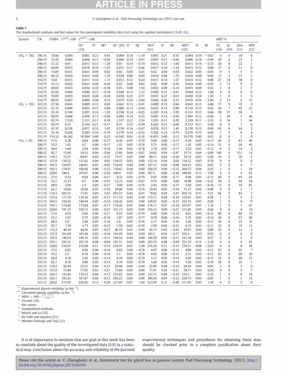
Table 7The standardized residuals and Hat values for the investigated solubility data [6,8] using the applied correlations [18,20–22].

System T/K P/MPa cexp⁎×100 ccalc⁎⁎×100 ARDa/%

Chb

[18]Hc SRd ALe [20] H SR dVAf

[21]H SR MSTg

[22]H SR Ch

[18]AL[20]

dVA[21]

MST[22]

CH4 + TEG 298.15 16.06 0.004 0.003 0.21 0.41 0.004 0.18 −1.10 0.003 0.21 0.35 0.004 0.19 −0.63 6 0 10 8298.15 32.43 0.006 0.008 0.17 −0.90 0.006 0.16 −0.97 0.007 0.17 −0.66 0.006 0.18 −0.49 29 2 23 1298.15 51.32 0.01 0.013 0.13 −1.29 0.01 0.14 −0.74 0.013 0.12 −1.64 0.011 0.14 −0.73 28 0 22 1298.15 64.85 0.015 0.018 0.10 −1.25 0.015 0.11 −0.46 0.017 0.10 −1.24 0.015 0.12 0.08 17 0 11 0298.15 74.85 0.021 0.021 0.09 0.02 0.02 0.09 0.21 0.02 0.09 0.05 0.022 0.09 −0.03 0 5 5 4298.15 86.12 0.029 0.025 0.08 1.70 0.028 0.08 0.64 0.024 0.08 1.76 0.029 0.08 0.94 13 3 17 1316.75 18.8 0.015 0.011 0.14 1.71 0.013 0.12 0.24 0.011 0.14 1.57 0.015 0.12 0.08 27 14 30 0316.75 33.13 0.022 0.021 0.09 0.44 0.02 0.09 0.62 0.02 0.09 0.50 0.024 0.09 −0.45 5 11 9 6316.75 49.03 0.033 0.034 0.10 −0.36 0.03 0.08 1.54 0.032 0.09 −0.14 0.035 0.09 0.22 2 8 2 7316.75 63.92 0.044 0.046 0.17 −0.78 0.044 0.13 1.12 0.044 0.17 −0.81 0.044 0.13 1.90 4 0 0 0316.75 75.05 0.055 0.056 0.28 −0.34 0.058 0.25 0.71 0.053 0.27 −0.03 0.058 0.24 1.20 1 6 3 5316.75 86.97 0.067 0.066 0.44 0.72 0.079 0.56 −2.64 0.064 0.45 0.31 0.078 0.54 −2.84 2 17 6 15

CO2 + TEG 323.15 27.58 0.041 0.009 0.15 0.66 0.041 0.15 −0.47 0.009 0.15 0.64 0.041 0.15 0.48 77 0 79 0323.15 41.37 0.096 0.053 0.15 0.99 0.089 0.15 −0.44 0.052 0.15 0.98 0.118 0.15 0.42 45 7 45 23323.15 55.16 0.149 0.207 0.14 −1.93 0.196 0.14 −0.65 0.205 0.14 −1.95 0.151 0.15 0.48 39 31 38 1323.15 68.95 0.688 0.698 0.13 −0.49 0.482 0.14 0.33 0.692 0.13 −0.50 1.002 0.13 −0.46 1 30 1 46323.15 82.74 2.319 2.311 0.11 0.18 1.537 0.12 2.54 2.291 0.11 0.20 3.339 0.11 −2.53 0 34 1 44323.15 96.53 8.31 8.334 0.21 −0.17 8.31 0.22 −0.29 8.263 0.21 −0.08 8.312 0.21 0.46 0 0 1 0333.15 41.37 0.136 0.077 0.15 1.45 0.136 0.14 −0.47 0.076 0.15 1.45 0.138 0.15 0.48 43 0 44 2333.15 55.16 0.266 0.285 0.14 −0.79 0.279 0.14 −0.52 0.282 0.14 −0.79 0.276 0.15 0.45 7 5 6 4333.15 110.32 16.542 16.584 0.80 0.22 16.542 0.81 −0.18 16.451 0.80 0.12 16.578 0.80 0.63 0 0 1 0

CO2 + EG 308.15 27.6 0.26 0.04 0.06 −0.17 0.26 0.05 −0.79 0.04 0.06 −0.17 0.38 0.05 −0.13 85 0 83 46308.15 55.2 1.01 0.7 0.06 −0.17 1.01 0.05 −0.78 0.75 0.06 −0.17 1.45 0.05 −0.14 31 0 26 43308.15 68.9 2.44 2.64 0.05 −0.18 2.44 0.05 −0.78 2.78 0.05 −0.17 2.54 0.05 −0.12 8 0 14 4308.15 82.7 13.86 34.15 0.04 −0.46 13.86 0.04 −0.67 34.85 0.04 −0.47 15.74 0.04 −0.09 146 0 151 14308.15 110.3 75.57 89.97 0.03 −0.37 75.57 0.03 0.00 90.71 0.03 −0.38 79.72 0.03 0.28 19 0 20 5308.15 137.9 134.22 121.62 0.04 0.02 134.22 0.03 0.00 122.16 0.04 0.02 134.22 0.03 0.78 9 0 9 0308.15 165.5 154.05 146.81 0.05 −0.05 154.05 0.04 0.00 147.12 0.05 −0.06 164.43 0.03 0.65 5 0 4 7308.15 193.1 170.61 168.46 0.06 −0.12 170.61 0.04 0.00 168.53 0.06 −0.12 200.73 0.04 0.25 1 0 1 18308.15 220.6 180.4 187.67 0.08 −0.26 180.4 0.05 0.00 187.5 0.08 −0.26 348.69 0.13 −3.49 4 0 4 93313.15 27.6 0.32 0.04 0.06 −0.17 0.32 0.05 −0.79 0.05 0.06 −0.17 0.46 0.05 −0.13 86 0 85 43313.15 55.2 12.33 0.7 0.06 −0.01 12.33 0.04 −0.67 0.76 0.06 0.00 18.98 0.04 −0.22 94 0 94 54313.15 68.9 2.69 2.3 0.05 −0.17 2.69 0.05 −0.78 2.43 0.05 −0.17 5.04 0.05 −0.18 15 0 10 87313.15 82.7 10.66 10.04 0.05 −0.16 10.66 0.04 −0.74 10.42 0.05 −0.16 11.37 0.04 −0.08 6 0 2 7313.15 110.3 495.21 77.91 0.03 5.81 495.21 0.45 6.25 78.82 0.03 5.81 505.74 0.31 3.51 84 0 84 2313.15 137.9 117.19 118.34 0.03 −0.17 117.19 0.03 0.59 119.11 0.04 −0.18 120.41 0.03 0.58 1 0 2 3313.15 165.5 150.26 149.44 0.05 −0.14 150.26 0.04 0.00 149.97 0.05 −0.15 163.15 0.03 0.56 1 0 0 9313.15 193.1 174.42 175.84 0.07 −0.17 174.42 0.05 0.00 176.11 0.07 −0.18 255.97 0.07 −1.10 1 0 1 47313.15 220.6 191.15 199.12 0.09 −0.27 191.15 0.05 0.00 199.12 0.09 −0.27 211.05 0.05 0.66 4 0 4 10323.15 27.6 0.52 0.05 0.06 −0.17 0.52 0.05 −0.79 0.06 0.06 −0.16 0.62 0.05 −0.13 90 0 89 19323.15 55.2 1.67 0.73 0.06 −0.16 1.67 0.05 −0.77 0.78 0.06 −0.16 2.35 0.05 −0.14 56 0 53 40323.15 68.9 2.9 2.06 0.05 −0.16 2.9 0.05 −0.78 2.17 0.05 −0.16 3.56 0.05 −0.13 29 0 25 23323.15 82.7 7.39 5.73 0.05 −0.15 7.39 0.05 −0.70 5.99 0.05 −0.15 8.33 0.05 −0.11 22 0 19 13323.15 110.3 40.19 44.36 0.03 −0.23 40.19 0.03 −0.59 45.15 0.03 −0.23 42.07 0.04 0.09 10 0 12 5323.15 137.9 101.69 101.44 0.03 −0.16 101.69 0.03 0.59 102.2 0.03 −0.17 102.2 0.03 0.55 0 0 0 0323.15 165.5 149.54 146.16 0.05 −0.11 149.54 0.04 0.00 146.59 0.05 −0.11 161.58 0.03 0.57 2 0 2 8323.15 193.1 191.51 183.74 0.08 −0.04 191.51 0.05 0.00 183.75 0.08 −0.04 351.33 0.13 −3.18 4 0 4 83323.15 220.6 216.47 216.68 0.11 −0.15 216.47 0.07 1.20 216.26 0.11 −0.15 276.31 0.08 −0.23 0 0 0 28333.15 27.6 0.82 0.06 0.06 −0.16 0.82 0.05 −0.78 0.07 0.06 −0.16 0.88 0.05 −0.13 93 0 92 7333.15 55.2 2.1 0.78 0.06 −0.16 2.1 0.05 −0.78 0.83 0.06 −0.15 2.31 0.05 −0.12 63 0 60 10333.15 68.9 4.18 2.02 0.05 −0.14 4.18 0.05 −0.74 2.12 0.05 −0.14 5.05 0.05 −0.13 52 0 49 21333.15 82.7 6.76 4.86 0.05 −0.15 6.76 0.05 −0.70 5.06 0.05 −0.14 7.26 0.05 −0.10 28 0 25 7333.15 110.3 26.44 25.21 0.04 −0.15 26.44 0.04 −0.44 25.69 0.04 −0.16 26.44 0.04 0.05 5 0 3 0333.15 137.9 73.84 77.02 0.03 −0.21 73.84 0.03 0.00 77.41 0.03 −0.21 78.71 0.03 0.24 4 0 5 7333.15 165.5 131.82 132.53 0.04 −0.17 131.82 0.03 0.00 132.31 0.04 −0.16 155.2 0.03 0.16 1 0 0 18333.15 193.1 183.23 181.87 0.08 −0.13 183.23 0.05 0.00 180.86 0.07 −0.12 228.73 0.05 −0.07 1 0 1 25333.15 220.6 217.05 225.85 0.13 −0.28 217.05 0.07 1.20 223.99 0.12 −0.26 217.05 0.05 1.36 4 0 3 0

⁎ Experimental glycols solubility (g dm−3).⁎⁎ Calculated glycols solubility (g dm−3).a ARD% ¼ 100� ccalc−c expj j

c exp .b Chrastil [18].c Hat values.d Standardized residuals.e Adachi and Lu [20].f del Valle and Aguilera [21].g Mèndez-Santiago and Teja [22].


It is of importance to mention that our goal in this work has beento conclude about the quality of the investigated data [6,8] in a statis-tical way. Conclusion about the accuracy and reliability of the pursued


experimental techniques and procedures for obtaining these datashould be checked prior to a complete justification about theirquality.





5. Conclusion

The Leveragemathematical strategy [13–15] was applied to evaluatethe experimental solubility data of ethylene/triethyleneglycols in super-critical CO2 ormethane so called as “glycol loss” data [6,8]. The graphicalmethod was performed on the basis of the Hat matrix and theWilliamsplot [13–15]. Three existing solubility datasets from the literature [6,8]were represented by four recommended [4] Chrastil-type correlations[18,20–22] to undertake the evaluation process. The results indicatethat:

I. The applied correlations are valid and statistically correct;II. One point from the solubility data of EG in supercritical CO2 is

found to be out of the applicability domain of the Adachi andLu [20] and Mèndez-Santiago and Teja [22] correlations, and

III. One experimental solubility data point from the dataset of theEG + CO2 system can be designated as suspended experimentaldatum, which has been detected using all of the applied correla-tions [18,20–22]. Furthermore, two data points evaluated usingthe Mèndez-Santiago and Teja correlation [22] may be declaredas the outliers.

References

[1] E.D. Sloan, C.A. Koh, Clathrate Hydrates of Natural Gases, third ed. CRC Press,Taylor & Francis Group, New York, 2008.

[2] E.G. Hammerschmidt, Formation of gas hydrates in natural gas transmission lines,Industrial and Engineering Chemistry Research 26 (1934) 851–855.

[3] A. Eslamimanesh, A.H. Mohammadi, D. Richon, P. Naidoo, D. Ramjugernath,Application of gas hydrate formation in separation processes: a review of exper-imental studies, Journal of Chemical Thermodynamics 46 (2012) 62–71.

[4] A. Eslamimanesh, A.H. Mohammadi, M. Yazdizadeh, D. Richon, Chrastil-typeapproach for representation of glycol loss in gaseous system, Industrial and Engi-neering Chemistry Research 50 (2011) 10373–10379.

[5] A.H. Mohammadi, A. Eslamimanesh, M. Yazdizadeh, D. Richon, Glycol loss in agaseous system: thermodynamic assessment test of experimental solubilitydata, Journal of Chemical and Engineering Data 56 (2011) 4012–4016.


[6] D. Jerinić, J. Schmidt, K. Fischer, L. Friedel, Measurement of the triethylene glycolsolubility in supercritical methane at pressures up to 9 MPa, Fluid Phase Equilibria264 (2008) 253–258.

[7] J.N.J.J. Lammers, Phase behavior of glycol in gas pipeline calculated, Oil and GasJournal 89 (1991) 50–55.

[8] T. Yonemoto, T. Charoensombut-Amon, R. Kobayashi, Solubility of triethyleneglycol in supercritical CO2, Fluid Phase Equilibria 55 (1990) 217–229.

[9] Y. Adachi, P. Malone, T. Yonemoto, R. Kobayashi, Glycol vaporization losses insuper-critical CO2, GPA Research Report RR-98, 1986.

[10] A.H. Mohammadi, D. Richon, Gas hydrate phase equilibrium in the presenceof ethylene glycol or methanol aqueous solution, Industrial and EngineeringChemistry Research 49 (2010) 8865–8869.

[11] A.H. Mohammadi, A. Eslamimanesh, D. Richon, Wax solubility in gaseous system:thermodynamic consistency test of experimental data, Industrial and EngineeringChemistry Research 50 (2011) 4731–4740.

[12] A. Eslamimanesh, A.H. Mohammadi, D. Richon, Thermodynamic consistency testfor experimental solubility data in carbon dioxide/methane + water systeminside and outside gas hydrate formation region, Journal of Chemical and Engi-neering Data 56 (2011) 1573–1586.

[13] P.J. Rousseeuw, A.M. Leroy, Robust Regression and Outlier Detection, John Wiley& Sons, New York, 1987.

[14] C.R. Goodall, Computation using the QR decomposition, Handbook in Statistics,vol. 9, Elsevier/North-Holland, Amsterdam, 1993.

[15] P. Gramatica, Principles of QSAR models validation: internal and external, QSARand Combinatorial Science 26 (2007) 694–701.

[16] A. Eslamimanesh, F. Gharagheizi, A.H. Mohammadi, D. Richon, A novel method forevaluation of asphaltene precipitation titration data, Chemical EngineeringScience 78 (2012) 181–185.

[17] A. Eslamimanesh, F. Gharagheizi, A.H. Mohammadi, D. Richon, A statistical methodfor evaluation of the experimental phase equilibrium data of simple clathratehydrates, Chemical Engineering Science 80 (2012) 402–408.

[18] J. Chrastil, Solubility of solids and liquids in supercritical gases, Journal of PhysicalChemistry 86 (1982) 3016–3021.

[19] S. Ismadji, S.K. Bhatia, Solubility of selected esters in supercritical carbon dioxide,Journal of Supercritical Fluids 27 (2003) 1–11.

[20] Y. Adachi, C.Y. Lu, Supercritical fluid extraction with carbon dioxide and ethylene,Fluid Phase Equilibria 14 (1983) 147–156.

[21] J.M. del Valle, J.M. Aguilera, An improved equation for predicting the solubility ofvegetable oils in supercritical CO2, Industrial and Engineering Chemistry Research27 (1988) 1551–1559.

[22] J. Méndez-Santiago, A.S. Teja, The solubilities of solids in supercritical fluids, FluidPhase Equilibria 158 (1999) 501–510.


