Axioms for Real-Time Logics�J.-F. Raskin P.-Y. SchobbensComputer Science InstituteUniversity of Namur - BelgiumMarch 1, 1998AbstractThis paper presents a complete axiomatization of fully decidable propositional real-timelinear temporal logics with past: the Event Clock Logic (EventClockTL) and the Metric In-terval Temporal Logic with past (MetricIntervalTLP ). The completeness proof consists of ane�ective proof building procedure for EventClockTL. It is structured to yield a similar axiom-atization and procedure for interesting fragments of this logic: the linear temporal logic ofthe real numbers (LTR), the fragment with only one clocks, with only past clocks.1 IntroductionMost real-time systems (nuclear plant control, plane control, etc.) are critical, and thereforedeserve to be speci�ed the with mathematical precision. To this end, real-time temporal logics [6]have been proposed as the basis of speci�cation languages such as TRIO [12], Albert [8, 11]. Theyuse real numbers for time, which has advantages for speci�cation and compositionality. Severalsyntaxes are possible to deal with real-time: freeze quanti�cation [4, 13], explicit clocks in a �rst-order temporal logic [19] and time-bounded operators [15, 16] studied here. The propositionalfragment of these logics (MetricTLR+) is undecidable, but becomes decidable with mild restrictions(MetricIntervalTL[3]), allowing automatic reasoning, animation, and veri�cation of programs usingautomata-based techniques. However, when the speci�cation is large or when it contains �rst-order parts, a mixture of automatic and manual proof generation is more suitable. Unfortunately,the current automatic reasoning techniques (based on timed automata) do not provide explicitproofs. This is why the axiomatization of these logics is cited as an important open question in[6].We bridge this gap by providing complete axiom systems for decidable real-time logics, anda proof-building procedure. We build these axiom systems by considering increasingly complexlogics: LTR [7], EventClockTLwith past clocks only, EventClockTLwith past and future clocks (alsocalled SCL [20]), MetricIntervalTL[3] with past and future operators [5].2 Models of real-timeAs time domain, we choose the nonnegative reals R+ . This dense domain is natural and givescompositionality [7], full abstractness [7], stuttering independence [1], facilitates re�nement. Toavoid Zeno's paradox, we add to our models the condition of �nite variability [7] (condition (3)below): only �nitely many state changes can occur in a �nite amount of time.An interval I � R+ is a convex non-empty subset of the nonnegative reals. Given t 2 R+ , wefreely use notation such as t+ I for the interval ft0 j exists t00 2 I with t0 = t+ t00g, t > I for the�This work was partially supported by the Belgian National Fund for Scienti�c Research (FNRS), by the Eu-ropean Commission under WGs Aspire (22704) and Fireworks (23531) and by Belgacom, and by the PortugeseFundation for Science and Technology (FCT). 1

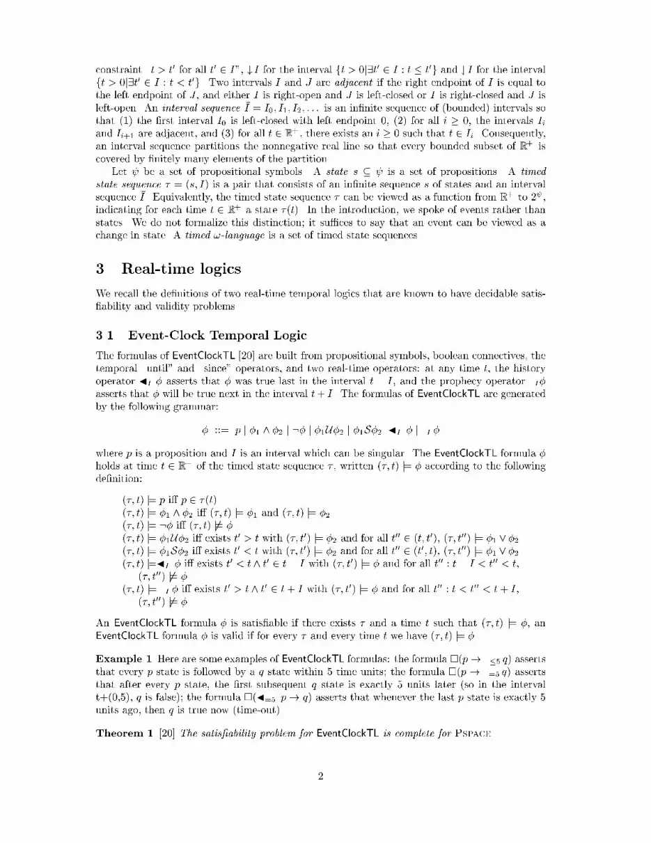
constraint \t > t0 for all t0 2 I", # I for the interval ft > 0j9t0 2 I : t � t0g and � I for the intervalft > 0j9t0 2 I : t < t0g. Two intervals I and J are adjacent if the right endpoint of I is equal tothe left endpoint of J , and either I is right-open and J is left-closed or I is right-closed and J isleft-open. An interval sequence �I = I0; I1; I2; : : : is an in�nite sequence of (bounded) intervals sothat (1) the �rst interval I0 is left-closed with left endpoint 0, (2) for all i � 0, the intervals Iiand Ii+1 are adjacent, and (3) for all t 2 R+ , there exists an i � 0 such that t 2 Ii. Consequently,an interval sequence partitions the nonnegative real line so that every bounded subset of R+ iscovered by �nitely many elements of the partition.Let be a set of propositional symbols. A state s � is a set of propositions. A timedstate sequence � = (�s; �I) is a pair that consists of an in�nite sequence �s of states and an intervalsequence �I . Equivalently, the timed state sequence � can be viewed as a function from R+ to 2 ,indicating for each time t 2 R+ a state �(t). In the introduction, we spoke of events rather thanstates. We do not formalize this distinction; it su�ces to say that an event can be viewed as achange in state. A timed !-language is a set of timed state sequences.3 Real-time logicsWe recall the de�nitions of two real-time temporal logics that are known to have decidable satis-�ability and validity problems.3.1 Event-Clock Temporal LogicThe formulas of EventClockTL [20] are built from propositional symbols, boolean connectives, thetemporal \until" and \since" operators, and two real-time operators: at any time t, the historyoperator JI � asserts that � was true last in the interval t � I , and the prophecy operator .I�asserts that � will be true next in the interval t+ I . The formulas of EventClockTL are generatedby the following grammar:� ::= p j �1 ^ �2 j :� j �1U�2 j �1S�2 jJI � j .I �where p is a proposition and I is an interval which can be singular. The EventClockTL formula �holds at time t 2 R+ of the timed state sequence � , written (�; t) j= � according to the followingde�nition:(�; t) j= p i� p 2 �(t)(�; t) j= �1 ^ �2 i� (�; t) j= �1 and (�; t) j= �2(�; t) j= :� i� (�; t) 6j= �(�; t) j= �1U�2 i� exists t0 > t with (�; t0) j= �2 and for all t00 2 (t; t0), (�; t00) j= �1 _ �2(�; t) j= �1S�2 i� exists t0 < t with (�; t0) j= �2 and for all t00 2 (t0; t), (�; t00) j= �1 _ �2(�; t) j=JI � i� exists t0 < t ^ t0 2 t� I with (�; t0) j= � and for all t00 : t� I < t00 < t,(�; t00) 6j= �(�; t) j= .I � i� exists t0 > t ^ t0 2 t+ I with (�; t0) j= � and for all t00 : t < t00 < t+ I ,(�; t00) 6j= �An EventClockTL formula � is satis�able if there exists � and a time t such that (�; t) j= �, anEventClockTL formula � is valid if for every � and every time t we have (�; t) j= �.Example 1 Here are some examples of EventClockTL formulas: the formula �(p! .�5 q) assertsthat every p state is followed by a q state within 5 time units; the formula �(p ! .=5 q) assertsthat after every p state, the �rst subsequent q state is exactly 5 units later (so in the intervalt+(0,5), q is false); the formula �(J=5 p! q) asserts that whenever the last p state is exactly 5units ago, then q is true now (time-out).Theorem 1 [20] The satis�ability problem for EventClockTL is complete for Pspace.2

3.2 Metric-Interval Temporal LogicThe formulas of MetricIntervalTL [3] are built from propositional symbols, boolean connectives,and the time-bounded \until" and \since" operators:� ::= p j �1 ^ �2 j :� j �1UI �2 j �1SI �2where p is a proposition and I is a nonsingular interval. The MetricIntervalTL formula � holds attime t 2 R+ of the timed state sequence � , written (�; t) j= � according to the following de�nition(the propositional and boolean clauses are as for EventClockTL):(�; t) j= �1UI �2 i� exists t0 2 t+ I with (�; t0) j= �2 and for all t00 : t < t00 < t0 (�; t0) j= �1(�; t) j= �1SI �2 i� exists t0 2 t� I with (�; t0) j= �2 and for all t00 : t0 < t00 < t (�; t0) j= �1A MetricIntervalTL formula �, then, de�nes the timed !-language that contains all timed statesequences � with (�; 0) j= �.Example 2 Here are some examples of MetricIntervalTL formulas: the formula �(q ! rS�5 p)asserts that every q state is preceded by a p state of time di�erence at most 5, and all intermediatestates are r states; the formula �(p! �[5;6)q) asserts that every p state is followed by a q state ata time di�erence of at least 5 and less than 6 time units. The formula .[5;6)q of EventClockTL isstronger than �[5;6)q: .[5;6)q that the �rst occurrence of a q-state is at a distance of at least 5 andand less than 6 while �[5;6)q expresses that there is some (not necessarily �rst) q-state in t+[5; 6).Theorem 2 [3] The satis�ability and validity problems for MetricIntervalTL are complete for Ex-pspace.3.3 AbbreviationsIn the sequel we use the following abbreviations:� �1U�2 � �1U(0;1)�2, the untimed \Until" of MetricIntervalTL. Let us note that �1U�2 ��1U�2 ^ B�1 (B is de�ned below); 1� �1U+�2 � �1 ^ �1U�2, the \Until" re exive for its �rst argument;� �1U��2 � �2 _ �1U+�2, the \Until" re exive for its two arguments;� J � � ?U�, meaning \just after in the future" or \arbritrarily closed in the future";� �� � >U�, meaning \eventually in the future";� �� � :�:�, meaning \always in the future";� their re exive counterparts: ��;��;� �1W�2 � �1U�2 _��1, meaning \unless";� its re exive counterparts: W+, W�.and the past counterpart of all those abbreviations:� �1S�2 � �1S(0;1)�2, the untimed \Since" of MetricIntervalTL. Let us note that �1S�2 ��1S�2 ^ J �1;� �1S+�2 � �1 ^ �1S�2, the \Since" re exive for its �rst argument;� �1S��2 � �2 _ �1S+�2, the \Since" re exive for its two arguments;1Let us note that the \Until" of EventClockTL and the \Until" of MetricIntervalTL are interde�nable, in fact, wealso have: �1U�2 � (�1 _ �2)U�2. 3

� B� � ?S�, meaning \just before in the past" or \arbritrarily closed in the past";� �� � >S�, meaning \eventually in the past";� �� � :�:�, meaning \always in the past";� their re exive counterparts: ��;��;� �1Z�2 � �1S�2 _��1, meaning \unless in the past";� its re exive counterparts: Z+, Z�.4 Axiomatization of EventClockTL4.1 AxiomsIn Subsection 4.3, we will present a proof-building procedure for EventClockTL. In this section, wesimply collect the axioms used in the procedure, and present their intuitive meaning. Our logicsare symmetric for past and future (a duality that we call the \mirror principle"), except thattime begins but does not end: therefore the axioms will be only written for the future, but withthe understanding that their mirror images, obtained by replacing U by S, . by J, etc. are alsoaxioms. This does not mean that we have an axiomatization of the future fragment of these logics:our axioms make past and future interact, and we believe that this interaction is unavoidable.We use the rule of inference: �$ �( )�(�) (RE)All propositional tautologiesFor the non-metric part, we use the following axioms and their mirror images::( U?) (N)�U( ^ 0)! �U (K)J ( ^ �)$ J ^ J � (JA)B> ! (B:�$ :B�) (BN)J ( U�)$ U� (JU)J ( S�) $ J � _ (J ^ (� _ ( ^ S�))) (JS) U�$ J ( U��) (UJ)�U ! � (SF)�(( ^ J> ! J ) ^ (B ! ))! (J ! � ) (JI)They mainly make use of the J operator, because as we shall see, it corresponds to the transitionrelation of our structure. Axiom (N) is the usual necessitation or modal generalisation rule,expressed as an axiom. Similarly,(K) is the usual weakening principle, expressed in a slightly non-classical form. (JA), (BN) allow to distribute J with boolean operators. Note that the validityof (BN) requires �nite variability. (JU), (JS) describe how the U and S operators are transmittedover interval boundaries. (UJ) gives local consistency conditions over this transmission. (SF)ensures eventuality when combined with (JI). It can also be seen as weakening the left side ofthe U to >. The induction axiom (JI) is essential to express �nite variability: If a property istransmitted over interval boundaries, then it will be true at any point: said otherwise, any pointis reached by crossing �nitely many interval boundaries.The axioms below express that time begins (B) but has no end (JT):��:B> (BE)J> (JT)4

We have written the other axioms so that they are independent of the begin or end axioms, inorder to deal easily with other time domains. For instance, to deal with the (positive and negative)reals numbers, we just use the mirror of (JT) instead of (BE).Remark 1 It is easy to check that the proof of completeness of Subsection 4.3 only uses the axiomsabove for a formula without real-time; therefore they form a complete axiomatization of the logic ofthe reals with �nite variability, de�ned as LTR in [7]. The system proposed in [7] is unfortunatelyunsound, redundant and incomplete. Indeed, axiom F5 of [7] is unsound (this is a simple typo);axiom F7 can be deduced from axiom F8; and the system cannot derive the induction axiom (JI).To see this last point, take the structure formed by R+ followed by R, with �nite variability: itsatis�es the system of [7] but not the induction axiom. Thus this valid formula cannot be provedin their system.For the real-time part, we �rst describe the static behaviour; intersection, union of intervalscan be translated into conjunction, disjunction due to the fact that there is a single next event:.I[J�$ .I� _ .J� (OR).I\J�$ .I� ^ .J� (AND): .=0 � (F).>0 $ � (P-S).�m+n�$ .�m .�n � (NLE).<m+n�$ .<m .�n � (NLT)The next step of the proof is to describe how a single real-time .I� evolves over time, using Jand B. We use (LO) to reduce left-open events to the easier case of left-closed ones.:(:�U�)! (.[l;m)J �$ .(l;m)�) (LO):J .=m (J=): U ! (J .<m $ .�m ) (JP)B .<m $ ((.<m _ _ B ) ^ B>) (JH)J ! .<m (J-P)These axioms are complete for formulae where the only real-time operators are predictionoperators .I� and they all track the same (qualitative) formula �. For a single history trackedformula, we use the mirror of the axioms plus an axiom expressing that the future time is in�nite,so that any bound will be exceeded: ! (� _ � J>m ) (ER)As soon as several such formulae are present, we cannot just combine their individual behaviour,because the .;J have to evolve synchronously (with the common implicit real time). We use afamily of \shift" and \order" axioms and their mirrors to express this common speed. The \shift"axioms say that the ordering the ticks should be preserved: the main antecedent : J=1 U� J=1 �states that � will tick before ; in this case the events shall be in the same order: :�S . Theside conditions ensure that the clocks were active in the meantime. The \order" axioms states asimilar property: (OHH) says that if last � was less than 1 ago, and was before, than last was less than 1 ago.J�1 ^ : U� J=1 � ^ : J=1 U� J=1 �! :�S (SHH)(.<1 _ ) ^ : U��! : .=1 �Z .=1 _ : .=1 �Z (SPP)(.<1 _ ) ^ : U� J=1 �! :�Z .=1 _ :�Z (SPH)J�1 ^ : U�� ^ : J=1 U��! : .=1 �S (SHP)J<1 � ^ :�S ! J<1 (OHH)J<1 ^ : S .=1 �! .<1� ^ :� (OHP)5

4.2 TheoremsWe also use in the proof some derived rules and theorems:� the rule of Modus Ponens is derivable from replacement as follows: from A we deducepropositionally A $ >; by replacement we replace A by > in A ! B giving > ! B whichyields propositionally B;� the rule of modal generalisation (also called necessitation) is derived from (RE) and (N).::�$ � (NN):B> ! (B�$ ?) (BB)JB�$ J � (JB)B ! B> (BT)JJ �$ J � (JJ)�> (ST)JI ! B> (HB):(: U )! : .=m � (N=):(: U )! (�J �$ ��) (SO).I�$ : .<I � ^ .#I (LOW)J (�1 _ �2)$ J �1 _ J �2 (JO).I�! .J� with (I � J) (MON)��1 ^ �2 ! ��1 (KA)4.3 Adequation of the axiomatic system for EventClockTLAs usual, the soundness of the system of axioms can be proved by a simple inductive reasoningon the structure of the axioms. We concentrate here on the more di�cult part of the adequationof the proposed axiomatic system: its completeness. As usual with temporal logic, we only haveweak completeness: for every valid formula of EventClockTL, there exists a �nite formal derivationin our axiomatic system for that formula. So if j= � then ` �. As often, it is more convenientto prove the contrapositive: every consistent EventClockTL formula is satis�able. Our logics aresymmetric for past and future (a duality that we call \mirror principle"), except that time beginbut does not end: therefore most explanations will be given for the future, but the careful readerwill check their applicability to the past as well.Our proof is divided in steps, that prove the completeness for increasing fragments of Event-ClockTL.1. We �rst deal with the qualitative part, without real-time. This part of the proof followsroughly the completeness proof of [18] for discrete-time logic.(a) We work with worlds that are built syntactically, by maximal consistent sets of formulae.(b) We identify the transition relation, and its syntactic counterpart: it was the \next"operator for discrete-time logic [18], here it is the J , expressing the transition from aclosed to an open interval, and B, expressing the transition from an open to a closedinterval.(c) We impose axioms describing the possible transitions for each operator.(d) We give an induction principle (JI) that extend the properties of local transitions toglobal properties.2. For the real-time part: 6

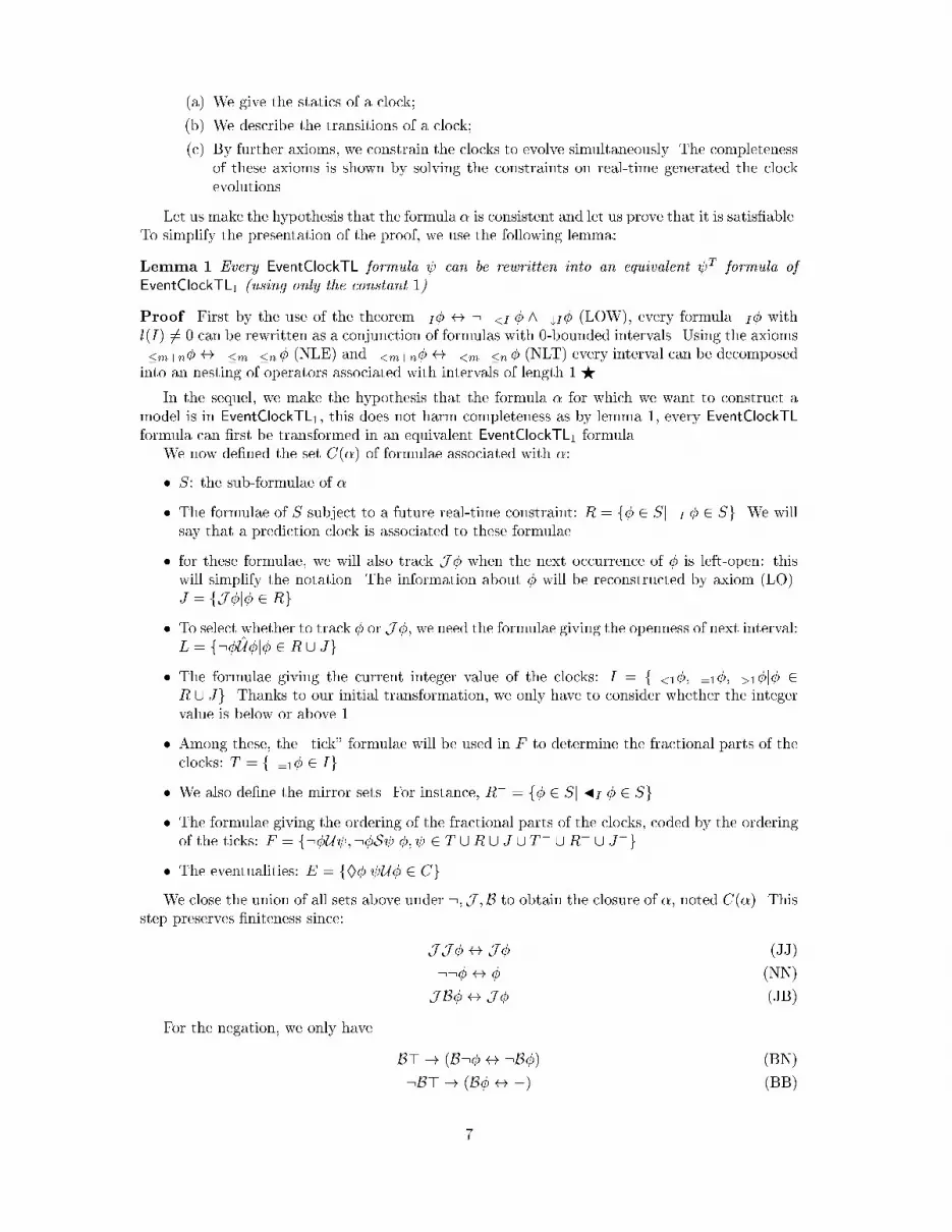
(a) We give the statics of a clock;(b) We describe the transitions of a clock;(c) By further axioms, we constrain the clocks to evolve simultaneously. The completenessof these axioms is shown by solving the constraints on real-time generated the clockevolutions.Let us make the hypothesis that the formula � is consistent and let us prove that it is satis�able.To simplify the presentation of the proof, we use the following lemma:Lemma 1 Every EventClockTL formula can be rewritten into an equivalent T formula ofEventClockTL1 (using only the constant 1).Proof. First by the use of the theorem .I� $ : .<I � ^ .#I� (LOW), every formula .I� withl(I) 6= 0 can be rewritten as a conjunction of formulas with 0-bounded intervals. Using the axioms.�m+n�$ .�m .�n � (NLE) and .<m+n�$ .<m .�n � (NLT) every interval can be decomposedinto an nesting of operators associated with intervals of length 1.FIn the sequel, we make the hypothesis that the formula � for which we want to construct amodel is in EventClockTL1, this does not harm completeness as by lemma 1, every EventClockTLformula can �rst be transformed in an equivalent EventClockTL1 formula.We now de�ned the set C(�) of formulae associated with �:� S: the sub-formulae of �.� The formulae of S subject to a future real-time constraint: R = f� 2 Sj .I � 2 Sg. We willsay that a prediction clock is associated to these formulae.� for these formulae, we will also track J � when the next occurrence of � is left-open: thiswill simplify the notation. The information about � will be reconstructed by axiom (LO).J = fJ �j� 2 Rg.� To select whether to track � or J �, we need the formulae giving the openness of next interval:L = f:�U�j� 2 R [ Jg.� The formulae giving the current integer value of the clocks: I = f.<1�; .=1�; .>1�j� 2R [ Jg. Thanks to our initial transformation, we only have to consider whether the integervalue is below or above 1.� Among these, the \tick" formulae will be used in F to determine the fractional parts of theclocks: T = f.=1� 2 Ig.� We also de�ne the mirror sets. For instance, R� = f� 2 Sj JI � 2 Sg.� The formulae giving the ordering of the fractional parts of the clocks, coded by the orderingof the ticks: F = f:�U ;:�S j�; 2 T [ R [ J [ T� [ R� [ J�g.� The eventualities: E = f��j U� 2 CgWe close the union of all sets above under :;J ;B to obtain the closure of �, noted C(�). Thisstep preserves �niteness since: JJ �$ J � (JJ)::�$ � (NN)JB�$ J � (JB)For the negation, we only have B> ! (B:�$ :B�) (BN):B> ! (B�$ ?) (BB)7

We only have two possible cases: if B> is true, we can move all negations outside and cancel them,except one. else, we know that all B are false. In each case, at most one B;J and one : areneeded.A Propositionally consistent structureA set of formula F � C(�) is complete w.r.t. C(�) if for all formula � 2 C(�), either � 2 F or:� 2 F ; it is propositionally consistent if (i) for all formulas �1; �2 2 C(�), �1 2 F or �2 2 F i��1 _ �2 2 F ; (ii) for all formula � 2 C(�), � 2 F i� :� 62 F . We call such a set a propositionalatom of C(�).We de�ne a �rst structure, which is a �nite graph, S = (A;R) where A is the set of allpropositional atoms of C( ) and R � A � A is the transition relation of the structure. R isde�ned by considering two subtransition relations:� R] represents the transition from a right-closed to a left-open interval;� R[ represents the transition from a right-open to a left-closed interval.Let A;B be propositional atoms. We de�ne� AR]B , 8J � 2 C(�);J � 2 A$ � 2 B;� AR[B , 8B� 2 C(�); � 2 A$ B� 2 B.The transition relation R is the union of R] and R[, i.e. R(A;B) i� either R](A;B) or R[(A;B).Now we can de�ne that the atom A is singular i� it contains a formula of the form � ^ :J �or symmetrically. Thus any atom containing a tick (.=1�) is singular. As a consequence, A issingular i� :AR]A i� :AR[A (this is expected since the logic is stuttering-insensitive), and thata singular state is only connected to non-singular states. A is initial i� it contains :B>. Thus itcontains no formula of the form: �1S�2 or JI �. It is singular, since it contains > ^ :B>. A ismonitored i� it contains �, the formula of which we check oating satis�ability.Any atom is exactly represented by the conjunction of the formulas that it contains. For anatom A, we write A for that formula, that formula is �nite by de�nition of A. By propositionalcompleteness, we have:Lemma 2 ` WA2A A.We de�ne the formula R(A) to be WBjARB B. WBjAR]B B can be simpli�ed to VJ�2A �,because in the propositional structure, all other members of a B are allowed to vary freely andthus cancel each other by the distribution rule.Lemma 3 ` A! JR](A).JR](A) = J WBjAR]B B = VJ�2A J �. Using (JA) we obtain the thesis.Dually, WBjAR[B B can be simpli�ed to V�2A B�. Therefore:Lemma 4 ` BA! R[(A).Now let R+ be transitive closure of R. Since R] � R+ , we have:Lemma 5 ` BA! R+(A).Similarly,Lemma 6 ` A! JR+(A).Using the disjunction rule for each reachable A, we obtain: ` R+(A) ! JR+(A) and `BR+(A)! R+(A). Now we can use the induction axioms provided by �nite variability, i.e.�(( !J ) ^ (B ! )) ! (J ! � ) and �(( ^ B> ! B ) ^ (J ! )) ! (B ! � ), usingnecessitation and modus ponens, we obtain:Lemma 7 ` A! �R+(A). 8

A EventClockTL-consistent structureWe say that an atom A is EventClockTL-consistent if it is propositionally consistent and con-sistent with the axioms and rules given in Subsection 4.1. Now, we consider the structureS = (A; R), where A is the subset of propositional atoms that are EventClockTL-consistent andR = f(A;B)jR(A;B) and A;B 2 Ag. Note that the lemmas above are still valid in the structureS as only inconsistent atoms are suppressed. We now investigate more deeply the properties ofthe structure S and show how we can prove from that structure that the consistent formula � issatis�able.Amaximally strongly connected substructure (MSCS) D is a set of atomsD � A of the structureS such that (i) for all D1; D2 2 D, R+(D1; D2) and R+(D2; D1), i.e. every atom can reach theother atoms of the set D and conversely, and (ii) for all D1; D2 2 A such that (D1; D2) 2 R+ and(D2; D1) 2 R+ and D1 2 D then D2 2 D, i.e. D is maximal. A MSCS D is called initial if for all(D1; D2) 2 R and D2 2 D then D1 2 D, i.e. D has no incoming edges. Conversely, a MSCS D iscalled �nal if for all (D1; D2) 2 R and D1 2 D then D2 2 D, i.e. D has no outgoing edges.Lemma 8 Every �nal MSCS D of the structure S is self-ful�lling, i.e. for every formula of theform �1U�2 2 A with A 2 D, there exists B 2 D such that �2 2 B.Proof. Let us make the hypothesis that there exists �1U�2 2 A with A 2 D and for all B 2 D,�2 62 B. By lemma ` A ! �VBjR+(A;B) B (lemma 7), axiom ��1 ^ �2 ! ��1 (KA) and apropositional reasoning, we conclude ` A ! �:�2. Using the axiom (S-F) and the hypothesisthat �1U�2 2 A, we obtain ` A ! ��2 and by de�nition of �, we obtain ` A ! :�:�2 incontradiction with ` A! �:�2 which is impossible since A is, by hypothesis, consistent.FLemma 9 Every initial MSCS D of the structure S contains an initial atom, i.e. there existsA 2 D such that B> 62 A.Proof. By de�nition of initial MSCS, we know that for all (D1; D2) 2 R+ and D2 2 D, thenD1 2 D. Let us make the hypothesis that for all D 2 D, B> 2 D. By the mirror of lemma 7` A ! �VBjR+(B;A) B we conclude that ` A ! �B>, but as A is a consistent atom by axiom(A9), we know that �:B> 2 A, thus we obtain a contradiction since �� � :�:�.FIn the sequel, we concentrate on particular paths, called runs, of the structure S . A run ofthe structure S = (A; R) is an in�nite sequence � = A0A1 : : : (An : : : An+m)! : : : , paired with anin�nite sequence of intervals �I = I0I1 : : : In : : : such that:1. Initiality: A0 is an initial atom;2. Consecution: for every i � 0, (Ai; Ai+1) 2 R;3. Singularity: for every i � 0, if Ai is a singular atom then Ii is singular;4. Alternation: I0I1 : : : In : : : alternates between singular and open intervals, i.e. I0 is singular,and for all i > 0, Ii is singular i� Ii�1 is open, Ii is open i� Ii�1 is singular;5. Eventuality: the set fAn; :::; An+mg is a �nal MSCS of the structure S.Note that the timing information provided in �I is purely qualitative (singular or open); thereforeany alternating sequence is adequate at this qualitative stage. Later, we will construct a speci�csequence satisfying also the real-time constraints.Lemma 10 R is total.Proof. We prove R] total, i.e. for all A 2 StructC; f�jJ � 2 Ag is consistent. Then it will beincluded in an atom. Assume it is not. We have then J �;J:� 2 A. Using (JA), (N) this yieldsa contradiction in A. (Note: the (JT) axiom is implicitly used in the de�nition of R, instead ofappearing here). F 9

Lemma 11 For every atom A of the structure S, for every alternating interval sequence �I, thereis a run (�; �I) that passes through A.Proof. First the alternation and singularity constraints can always be veri�ed by taking stutteringsteps when needed and by noting that in S two singular atoms are never linked by R. It remainsus to show that :1. Initiality, i.e. every atom of S is either initial or can be reached by an initial atom. Let usconsider an atom A, if A is initial then we are done, otherwise, let us make the hypothesis thatit can not be reached by an initial atom, it means: for all B such that R+(B;A) then :B> 62 B,so by propositional completeness B> 2 B. By lemma 7, we obtain ` A ! �B>. Using axiom(BE) and our hypothesis B>, through �:B>, we obtain a contradiction.2. Finality, i.e. every atom of S either is part of a �nal MSCS or can reach one of the �nal MSCSof S. It is a direct consequence of the fact that R is total and the fact that S is �nite.F A run (�; �I) of the structure S is semantically sound if it respects the following conditions:1. if �i is singular then Ii is singular;2. if �1U�2 2 �i then:� either Ai is singular and there exists j > i s.t. �2 2 Aj and for all k s.t. i < k < j,�1 2 Ak ;� or Ai is not singular and(a) either �2 2 Ai(b) or there exists j > i s.t. �2 2 Aj and for all k s.t. i � k < j, �1 2 Ak;3. if �1S�2 2 �i then:� either Ai is singular and there exists j < i s.t. �2 2 Aj and for all k s.t. j < k < i,�1 2 Ak ;� or Ai is not singular and(a) either �2 2 Ai(b) or there exists j < i s.t. �2 2 Aj and for all k s.t. j < k � i, �1 2 Ak;4. if .I�1 2 Ai then for all time t 2 Ii, there exists j � i s.t. �1 2 Aj and (t+ I) \ Ij 6= ; andt+ (< I \ Ij) = ;;5. if JI �1 2 Ai then for all time t 2 Ii, there exists j � i s.t. �1 2 Aj and (t� I)\ Ij 6= ; andt� (< I \ Ij) = ;.A semantically sound run is called an timed Hintikka sequence. Next, we show properties ofruns:Lemma 12 For every run (�; �I) of the structure S, with � = A0A1 : : : , for every Ai such that�� 2 Ai:� Ai is singular and there exists j > i such that � 2 Aj ;� Ai is non-singular and there exists j � i such that � 2 Aj .Proof. First let us prove the following properties of the transition relation R:� let R](A;B) and �� 2 A then either � 2 B or �� 2 B. In fact, recall that �� � >U�,and by de�nition of R], axiom �1U�2 $ J (�2 _ (�1 ^ �1U�2)) (UJ) and a propositionalreasoning, we obtain that >U� 2 A i� � 2 B or >U� 2 B;10

� let R[(A;B) and �� 2 A then either � 2 A, � 2 B or >U� 2 B. By de�nition of R[, axiomB(�1U�2)$ B�2 _ (B�1 ^ �2 _ (�1 ^ �1U�2)) mirror of (JS) and a propositional reasoning,we obtain � 2 A or � 2 B or >U� 2 B.By the two properties above, we have that if �� 2 Ai then either � appears in Aj with j > i ifAi is singular (and thus right closed), j � j if Ai is not singular (and thus associated with anopen interval) or � is never true and �� propagates for the rest of the run. But let us show thatthis last possibility is excluded by our de�nition of run. In fact, every run eventually loops into a�nal self-full�lling MSCS D. Then either the fatality � associated with �� is realized before thislooping or �� 2 D and by lemma 9 the fatality � 2 D and is thus eventually realized. FLemma 13 For every run (�; �I) of the structure S, for every position i in the run if �1U�2 2 Aithen the property 2 of timed Hintikka sequences is veri�ed, i.e:� either Ai is singular and there exists j > i s.t. �2 2 Aj and for all k s.t. i < k < j,�1 2 Ak;� or Ai is not singular and1. either �2 2 Aj2. or there exists j > i s.t. �2 2 Aj and for all k s.t. i � k < j, �1 2 Ak.Proof. By hypothesis we know that �1U�2 2 Ai and we �rst treat the case where Ai is singular.� By the axiom �1U�2 ! ��2 and lemma 12, we know that there exists j > i such that�2 2 Aj . Let us make the hypothesis that Aj is the �rst �2-atom after Ai.� It remains us to show that: for all k s.t. i < k < j, �1 2 Ak. We reason by induction on thevalue of k.{ Base case: k = i + 1. By hypothesis we have �1U�2 2 Ai and also AiR]Ai+1 (as Aiis right closed) and thus for all J � 2 Ai; � 2 Ai+1 by de�nition of R]. By axiom�1U�2 $ J (�1U�2), we conclude that �1U�2 2 Ai+1 and by axiom �1U�2 $ J (�2 _(�1 ^ J (�1U�2))), J (�1 _ �2)$ J �1 _ J �2, J (�1 ^ �2)$ J �1 ^ J �2, and the factthat by hypothesis �2 62 Ai+1, a propositional reasoning allows us to conclude that�1 2 Ai+1.{ Induction case: k = i + l with 1 < l < j � i. By induction hypothesis, we know that�1 2 Ak�1 and �1U�2 2 Ak�1, also :�2 2 Ak and :�2 2 Ak�1 as k < j (by hypothesisj is the �rst position after i where �2 is veri�ed). To establish the result, we reason bycase : (i) Ik is open and thus Ik�1 is singular and right closed. We have Ak�1R]Ak , andthus for all J � 2 C( );J � 2 Ai $ � 2 Ai+1 by de�nition of R]. As �1U�2 2 Ak�1 byinduction hypothesis and the axiom �1U�2 $ J (�1U�2), we conclude that �1U�2 2Ak. Using the axioms �1U�2 $ J (�2 _ (�1 ^ J (�1U�2))), J (�1 _ �2)$ J �1 _ J �2,J (�1 ^ �2) $ J �1 ^ J �2, and the fact that �2 62 Ak , and a proposition reasoning,we conclude that �1 2 Ak. (ii) Ik is closed which implies that Ik�1 is right open andAk�1R[Ak. By de�nition of R[ we have that for all B� 2 C( );B� 2 Ak $ � 2 Ak�1.So we have B(�1U�2);B:�2 2 Ak, by hypothesis k < j thus we have :�2 2 Ak. Usingthose properties, the axiom B(�1U�2)$ B�2_(B�1^(�2_(�1^�1U�2))), we concludethat �1 ^ �1U�2 2 Ak.We now have to treat the case where Ai is not singular. By the axiom �1U�2 ! ��2 and lemma 12we know that there exists a later atom Aj j � i such that �2 2 Aj . If j = i then �2 2 Ai and weare done. Otherwise j > i, and we must prove that for all k s.t. i � k < j, �1 2 Ak, this can bedone by the reasoning above.FWe now prove the reverse, i.e. every time that �1U�2 is veri�ed in an atom along the runthen �1U�2 appears in that atom. This lemma is not necessary for completeness but we use thisproperty in the lemmas over real-time operators.11

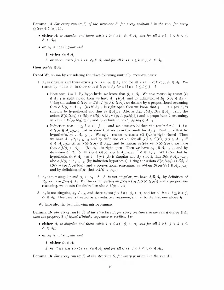
Lemma 14 For every run (�; I) of the structure S, for every position i in the run, for every�1U�2 2 C(�), if :� either Ai is singular and there exists j > i s.t. �2 2 Aj and for all k s.t. i < k < j,�1 2 Ak;� or Ai is not singular and1. either �2 2 Aj2. or there exists j > i s.t. �2 2 Aj and for all k s.t. i � k < j, �1 2 Ak.then �1U�2 2 Ai.Proof We reason by considering the three following mutually exclusive cases:1. Ai is singular and there exists j > i s.t. �2 2 Aj and for all k s.t. i < k < j, �1 2 Ak . Wereason by induction to show that �1U�2 2 Aj for all l s.t. 1 � l � j � i.� Base case: l = 1. By hypothesis, we know that �2 2 Aj . We now reason by cases: (i)if Aj�1 is right closed then we have Aj�1R]Aj and by de�nition of R], J �2 2 Aj�1.Using the axiom �1U�2 $ J �2_ (�1 ^�1U�2), we deduce by a propositional reasoningthat �1U�2 2 Aj�1. (ii) if Aj�1 is right open then we know that j � 1 > i (as Ai issingular by hypothesis) and thus �1 2 Aj�1. Also as Aj�1R[Aj , B�1 2 Aj . Using theaxiom B(�1U�2) $ B�2 _ (B�1 ^ (�2 _ (�1 ^ �1U�2))) and a propositional reasoning,we obtain B(�1U�2) 2 Aj and by de�nition of R[, �1U�2 2 Aj�1.� Induction case: 1 � l < i � j � 1 and we have established the result for l � 1, i.e.�1U�2 2 Aj�(l�1). Let us show that we have the result for Aj�l. First note that byhypothesis, �1 2 Aj�(l�1). We again reason by cases: (i) Ij�l is right closed. Thenwe have Aj�lR]Aj�(l�1) and by de�nition of R], for all J � 2 C( ), J � 2 Aj�l i�� 2 Aj�(l�1),thus J (�1U�2) 2 Aj�l and by axiom �1U�2 $ J (�1U�2), we havethat �1U�2 2 Aj�l. (ii) Aj�l is right open. Then we have Aj�lR[Aj�(l�1) and byde�nition of R[, for all B� 2 C( ), B� 2 Aj�(l�1) i� � 2 Aj�l. We know that byhypothesis, �1 2 Aj�l as j � l 6= i (Ai is singular and Aj�l not), thus B�1 2 Aj�(l�1),also �1U�2 2 Aj�(l�1) (by induction hypothesis). Using the axiom B(�1U�2)$ B�2 _(B�1 ^ (�1 ^ �1U�2)) and a propositional reasoning, we obtain B(�1U�2) 2 Aj�(l�1)and by de�nition of R[ that �1U�2 2 Aj�l.2. Ai is not singular and �2 2 Aj . As Ai is not singular, we have AiR]Ai, by de�nition ofR], we have J �2 2 Ai. By the axiom �1U�2 $ J �2 _ (�1 ^ J (�1U�2)) and a propositionreasoning, we obtain the desired result: �1U�2 2 Ai.3. Ai is not singular, �2 62 Aj , and there exists j > i s.t. �2 2 Aj and for all k s.t. i � k < j,�1 2 Ak. This case is treated by an inductive reasoning similar to the �rst one above.FWe have also the two following mirror lemmas:Lemma 15 For every run (�; �I) of the structure S, for every position i in the run if �1S�2 2 Aithen the property 3 of timed Hintikka sequences is veri�ed, i.e:� either Ai is singular and there exists j < i s.t. �2 2 Aj and for all k s.t. j < k < i,�1 2 Ak;� or Ai is not singular and1. either �2 2 Ai2. or there exists j < i s.t. �2 2 Aj and for all k s.t. j < k � i, �1 2 Ak;Lemma 16 For every run (�; I) of the structure S, for every position i in the run if :12

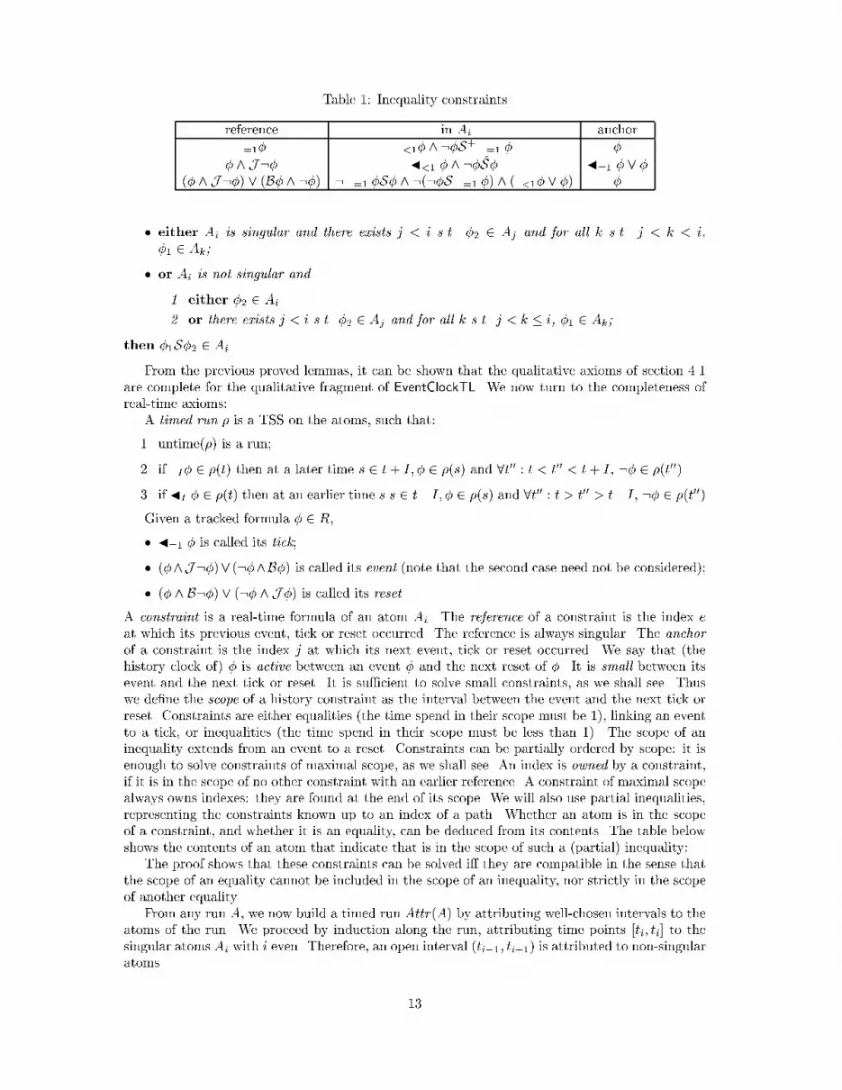
Table 1: Inequality constraintsreference in Ai anchor.=1� .<1� ^ :�S+ .=1 � �� ^ J:� J<1 � ^ :�S� J=1 � _ �(� ^ J:�) _ (B� ^ :�) : .=1 �S� ^ :(:�S .=1 �) ^ (.<1� _ �) �� either Ai is singular and there exists j < i s.t. �2 2 Aj and for all k s.t. j < k < i,�1 2 Ak;� or Ai is not singular and1. either �2 2 Ai2. or there exists j < i s.t. �2 2 Aj and for all k s.t. j < k � i, �1 2 Ak;then �1S�2 2 Ai.From the previous proved lemmas, it can be shown that the qualitative axioms of section 4.1are complete for the qualitative fragment of EventClockTL. We now turn to the completeness ofreal-time axioms:A timed run � is a TSS on the atoms, such that:1. untime(�) is a run;2. if .I� 2 �(t) then at a later time s 2 t+ I; � 2 �(s) and 8t00 : t < t00 < t+ I , :� 2 �(t00)3. if JI � 2 �(t) then at an earlier time s s 2 t�I; � 2 �(s) and 8t00 : t > t00 > t�I , :� 2 �(t00)Given a tracked formula � 2 R,� J=1 � is called its tick;� (�^J :�)_ (:�^B�) is called its event (note that the second case need not be considered);� (� ^ B:�) _ (:� ^ J �) is called its reset.A constraint is a real-time formula of an atom Ai. The reference of a constraint is the index eat which its previous event, tick or reset occurred. The reference is always singular. The anchorof a constraint is the index j at which its next event, tick or reset occurred. We say that (thehistory clock of) � is active between an event � and the next reset of �. It is small between itsevent and the next tick or reset. It is su�cient to solve small constraints, as we shall see. Thuswe de�ne the scope of a history constraint as the interval between the event and the next tick orreset. Constraints are either equalities (the time spend in their scope must be 1), linking an eventto a tick, or inequalities (the time spend in their scope must be less than 1). The scope of aninequality extends from an event to a reset. Constraints can be partially ordered by scope: it isenough to solve constraints of maximal scope, as we shall see. An index is owned by a constraint,if it is in the scope of no other constraint with an earlier reference. A constraint of maximal scopealways owns indexes: they are found at the end of its scope. We will also use partial inequalities,representing the constraints known up to an index of a path. Whether an atom is in the scopeof a constraint, and whether it is an equality, can be deduced from its contents. The table belowshows the contents of an atom that indicate that is in the scope of such a (partial) inequality:The proof shows that these constraints can be solved i� they are compatible in the sense thatthe scope of an equality cannot be included in the scope of an inequality, nor strictly in the scopeof another equality.From any run A, we now build a timed run Attr(A) by attributing well-chosen intervals to theatoms of the run. We proceed by induction along the run, attributing time points [ti; ti] to thesingular atoms Ai with i even. Therefore, an open interval (ti�1; ti+1) is attributed to non-singularatoms. 13

1. Base: We attribute the interval [0; 0] to the initial atom A0.2. Induction: we identify and solve the tightest constraint, that owns the current index i. Wede�ne e as the reference of this tightest constraint, by cases:(a) equality constraints:i. If there is an J=1 2 Ai there has been a last (singular) atom Ae containing before at time te.ii. Else, if B: ^ ^ : S .=1 2 Ai there has been a last atom Ae containing .=1 before Ai, at time te.We attribute [te + 1; te + 1] to Ai.(b) inequality constraints:i. Else, we compute the earliest reference e of the small clocks using table 1. ti hasto be between ti�2 and te + 1. We choose ti = (ti�2 + te + 1)=2.ii. Finally, when all clocks are unde�ned or blocked, we attribute (say) ti�2 + 1=2 toAi.The algorithm selects arbitrarily an equality constraint, but is still deterministic:Lemma 17 If two equality constraints have the same anchor i, their references e1; e2 are identical.Proof Four combinations of equality constraints are possible:� The �rst constraint is J=1 �{ The second constraint is J=1 : Ai contains : U� J=1 �;: J=1 U� J=1 � since itseventuality J=1 � is true now. It contains J=1 , and thus J�1 by (OR). We apply(SHH) to obtain :�S .We repeat this with ; � inverted to obtain : S�. These formula imply by Lemma 13that cannot occur before �, and conversely, thus they occur in the same atom.{ The second constraint is the event with : S .=1 : then Ai contains :�U� ;: J=1�U� since its eventuality is true now. It contains J=1 , and thus J�1 by (OR).We apply (SHP) to obtain : .=1 S�.Since Ai contains : U� J=1 � since its eventuality J=1 � is true now. We apply(SPH) to obtain :�Z .=1 _ :�Z . Since : S .=1 , we know that the �rst branchis true.These formula imply by Lemma 13 that cannot occur before �, and conversely, thusthey occur in the same atom.� The �rst constraint is the event � with :�S .=1 �:{ The second constraint is J=1 : This case is simply the previous one, with �; inverted.{ The second constraint is the event with : S .=1 : Ai contains : U�� since itseventuality � is true now. We apply (SPP) to obtain :.=1�Z(.=1 _ ). By : S.=1 ,the tick .=1 occurred.We repeat this with ; � inverted. These formula imply by Lemma 13 that .=1 cannotoccur before .=1�, and conversely, thus they occur in the same atom.F Solving an equation at its anchor also solves current partial inequations:Lemma 18 If Ai is in the scope of an inequation, and the anchor of an equation, then the referenceAj of the inequation is after the reference Ae of the equation.Proof. There are 3 possible forms of inequation in Ai (see table 4.3):14

1. J<1 ;: S 2 Ai:let j � i be its reference, i.e. 2 Aj . We must show that e < j. The equation can be:� J=1 � 2 Ai and � 2 Ae:Ai contains : U� J=1 �;: J=1 U� J=1 � since its eventuality J=1 � is true now. Weapply (SHH) to obtain :�S , meaning e � j. : S� 62 Ai, for otherwise we apply (OHH)yieldingJ<1 � 2 Ai contradicting J=1 � 2 Ai by (AND), so we conclude e < j.� �;:�S .=1 � 2 Ai and .=1� 2 Ae:by (SHP) : .=1 �S 2 Aj , so e � j. We cannot have the reverse : S .=1 �, for otherwisewe apply the mirror of (OPH) and deduce :� 2 Ai, so we conclude e < j.2. : .=1 S ^ :(: S .=1 ) ^ (.<1 _ ) 2 Ai:let j � i be its reference, i.e. � ^ J:� 2 Aj . Since .<1 2 Ai�1 and there is no intervening between j and i, the transition rules imply .<1 2 Aj+1 and thus .�1 2 Aj by (JH). Wemust show that e < j. The equation can be:� J=1 � 2 Ai and � 2 Ae:if .<1 _ 2 Ai, we apply (SPH) to obtain :�Z .=1 _ :�Z , which means e � j.The �rst branch is false by hypothesis as :(: S .=1 ) 2 Ai, since we deal with aninequality. Thus : .=1 2 Aj ; using .�1 2 Aj , .<1 2 Aj . Again because there areno intervening in (j; i), using lemma 14 we have : U J=1 � 2 Aj . Using the mirrorof (OHP), J<1 � ^ :� 2 Aj Thus j = e is impossible, since :� 2 Aj and � 2 Ae. Weconclude e < j.� �;:�S .=1 � 2 Ai and .=1� 2 Ae:so : U�� 2 Ai, and we use (SPP) to obtain : .=1 �Z .=1 _ : .=1 �Z . must occur�rst (:.=1 S 2 Ai), so the �rst case is excluded, giving :.=1 2 Aj ; using .�1 2 Aj ,.<1 2 Aj . Again because there are no intervening in (j; i), we have : U J=1 � 2 AjUsing the mirror of (OHH), .<1� 2 Aj . The second case is thus true, and means e � j.e = j is impossible, since .<1� 2 Aj ^ .=1� 2 Ae. We conclude e < j.3. .<1 ^ : S+ .=1 2 Ai and .=1 2 Aj :let j � i be its reference, i.e. .=1 2 Aj . We must show that e < j. The equation can be:� J=1 � 2 Ai and � 2 Ae:thus : U� J=1 � 2 Ai; by (SPH) :�Z .=1 _ :�Z 2 Ai. The �rst case is true as byhypothesis : S+ .=1 2 Ai (.=1 must occur before in the past), and gives e � j.� �;:�S .=1 � 2 Ai and .=1� 2 Ae:using (SPP), we obtain : .=1 �Z .=1 _ : .=1 �Z 2 Ai. The �rst case is true, byhypothesis, and gives e � j.We cannot assume e = j, because the mirror of lemma 17 then gives 2 Ai, contradicting: S+ .=1 2 Ai. We conclude e < j.FLemma 19 The sequence ti built by Attr is increasing.Proof. In the notation of the de�nition, this amounts to prove ti�2 < te + 1 when e is de�ned,since ti is either te + 1 or the middle point of (ti�2; te + 1). We prove both by induction on i:1. base case: i = 2. Either:� no constraint is active, e is unde�ned;� e = 0; te = 0; ti�2 = 0. We just have to prove 0 < 1.2. induction: We divide in cases according to the constraint selected at i � 2, whose reference iscalled ei�2:a. an equality: by lemmas 17, 18, its reference was before, i.e., ei�2 < e. By inductive hypothesis,ti is increasing: tei�2 < te. Thus ti�2 = tei�2 + 1 < te + 1.15

b. an inequality: Thus the reference ei�2 � ei, since it was obtained by sorting. By inductivehypothesis, ti is increasing: so tei�2 � te. By inductive hypothesis, ti�4 < tei�2 + 1. Thusti�2 = (ti�4 + tei�2 + 1)=2 < (tei�2 + 1 + tei�2 + 1)=2 = tei�2 + 1 � te + 1.FLemma 20 The sequence Attr(Run(A)) built above has �nite variability: for all t 2 R+ , thereexists an i � 0 such that t 2 Ii.Proof. Although there is no lower bound on the duration of an interval, we show that the timespend in each passage through the �nal cycle of Run(A) is at least 1=2. Thus any real number twill be reached before index 2tc, where c is the number of atoms in the �nal cycle. We divide incases:1. If the cycle contains an atom which is not in the scope of any constraint, the time spent therewill be 1=2.2. Else, the cycle contains constraints, and thus constraints of maximal scope. Let i be owned bysuch a constraint. The time spent in the scope of the constraint until i is at least 1=2: Since e isthe beginning of the scope of the constraint, and, ti�2 � te, and ti � (ti�2+te+1)=2 � te+1=2.Furthermore, note that the scope cannot be greater than one cycle: thus the time spent is acycle is at least 1=2.F This procedure correctly solves all constraints:Lemma 21 The interval attribution Attr transforms any run in a timed run.Proof. We show the two supplementary properties of a timed run:1. Let JI 2 �(t) = Ai. We must show that the next occurs in t� I . JI can be:a.J>1 : These constraints are automatically satis�ed because:� the mirror of the eventuality rule (P-S) guarantees has occurred: 9j < i 2 Aj ;� the transition rules (J axioms) guarantee that there is �rst a time where equality issatis�ed: 9k i < k < j ^ .=1 2 Ak;� the reset rule (CR) guarantees that satisfying the equality will entail satisfying thegreater-than constraint, since they refer to the same tracked event, and since the equalityis later.b.J=1 : Since this is an equality constraint, the algorithm Attr must have chosen an equalityconstraint with reference e. Thus ti = te + 1. By lemma 17, the reference event � is also inAe.c.J<1 : Let j � i be its reference, � 2 Aj . The constraint selected by Attr at i can be:� an equality, by lemma 18, its reference e < j, so that ti = te + 1 < tj + 1.� or the constraint chosen in Ai is an inequality. The pair J<1 2 Ai; 2 Aj is also aninequality in Ai: let f be its reference. The algorithm has selected the constraint withthe earliest reference e. Thus e � f � j � i, and ti < te + 1. Thus ti < tj + 1.2. Let .I 2 �(t) = Ai. We must show that the next occurs in t+ I . .I can be:a. .>1 : These constraints are automatically satis�ed because:� the eventuality rule (P-S) guarantees will occur: 9j < i 2 Aj ;� the transition rules (J axioms) guarantee that there is �rst a tick: 9k i < k < j^.=1 2Ak ;� the reset rule (CR) guarantees that satisfying the equality will entail satisfying thegreater-than constraint, since they refer to the same anchor event, and since the equalityis later.b. .=1 : let Aj contain the next event of . Since this is an equality constraint, the algorithmAttr must have chosen an equality constraint at Aj . By lemma 17, its reference is i. Thustj = ti + 1.c. .<1 : Let Aj contain the next event of . The constraint selected by Attr at j can be:16

� an equality by lemma 18 its reference e < i, so that tj = te + 1 < ti + 1.� or the constraint chosen in Aj is an inequality. The pair .<1 2 Ai; 2 Aj is also aninequality in Aj : let f be its reference. The algorithm has selected the constraint withthe earliest reference e. Thus e � f � i � j, and tj < te + 1. Thus tj < ti + 1.FTheorem 3 A timed run has the Hintikka property: 8� 2 C; � 2 �(t)$ (�; t) j= �.Proof. In lemma 14, we proved this for the (qualitative) runs. In theorem 21, we proved theimplication for the real-time operators. It remains only to prove the converse, which also resultsfrom timed: if .I� 62 �(t), by maximality : .I � 2 �(t) and thus either :�� 2 �(t) and the resultfollows by lemma 14, or .I� 2 �(t) and the result follows by lemma 21.FFinally, we obtain the desired theorem:Theorem 4 Every EventClockTL-consistent formula � is satis�able.Proof. if � is a EventClockTL-consistent formula then there exists an �-monitored atom A� inS . By lemma 11, there exists a set of runs � that pass throught A� and by the properties of theprocedure Attr, lemma 13, lemma 20 and lemma 21, at least one timed run (�; �I) 2 � has theHintikka property. It is direct to see that (� \ P; �I) is a model for � at time t 2 I� (the intervalof time associated to A� in (�; �I) ) and thus � is satis�able. F4.4 Comparison with the region automatonIn spirit, the procedure given above can be considered as building the automaton correspondingto a formula, and then constructing its region automaton. A region automaton will record theinteger value of each clock: this is coded here by formulas of the form .<1 .=1 ::: .=1 �. It willalso record the ordering of the fractional parts of the clocks: this is coded here by formulas ofthe form : .=1 ::: .=1 �U .=1 ::: .=1 �. There are some small di�erences, however: for simplicitywe maintain more information than needed, so that many atoms are redundant. For instance werecord the ordering of any two ticks, even if these ticks are not linked to the current value of theclock. This relationship is only inverted for a very special case: when a clock has no previous andno following tick, we need not and cannot maintain its fractional information since it will neverbe used, and thus cannot be expressed by a formula.The structure of atoms constructed here treats the eventualities in a di�erent spirit: here, weonly ensure that all atoms are part of a model, but there may be invalid paths in the graph ofatoms. It is immediate to add acceptance conditions to eliminate these spurious paths, and obtaina more classical automaton.5 Translating EventClockTLand MetricIntervalTLThe logics have been designed from a di�erent philosophical standpoint: MetricIntervalTLrestrictsthe undecidable logic MTL by \relaxing punctuality", i.e., forbidding to look at exact time values;EventClockTL, in contrast, forbids to look past next event in the future. However, we show herethat, surprisingly, they have the same expressive power. The power given by nesting connectivesallows to each logic to do some of its forbidden work.First, we suppress intervals containing 0:�UI $ _ (�UJ ) J [ f0g = I (R0)Then we replace bounded untils UI by simpler �I :�UI $ ^ ��I( _ �U )^ �<0I(�U )^ �<I(�)^ �I (RU)17

where the interval � I = ft > 0j8ti 2 I; t � tig, <0 I = ft � 0j8ti 2 I; t < tig.We suppress classical until using: �U $ �U( ^ B�) (UC)For in�nite intervals, we reduce the lower bound to 0 using�(l;1)�$ �(0;l]�� (IO)�[l;1)�$ �(0;l)�� (IC)For �nite intervals, we reduce the length of the interval to 1 using:�(0;u)�$ .<u� (DLT)�(0;u]�$ .�u� (DLE)When the application of this rule is not immediate, we reduce the length of the interval to 1 using:�I[J�$ �I� _ �J� (SOR)Then we use the following rules recursively until the lower bound is reduced to 0. Note that wehave written t > 0 instead of 1 for scalability.�(l;l+t)�$ �[l�t;l) .=t J � _ �(l�t;l) .=t � _�(l�t;l] .<t � (FOO)�(l;l+t]�$ �[l�t;l) .=t J � _ �(l�t;l] .=t � _�(l�t;l] .<t � (FOC)�[l;l+t)�$ �[l�t;l) .=t J � _ �[l�t;l) .=t � _�(l�t;l]�[0;t)� (FCO)�[l;l+t]�$ �[l�t;l) .=t J � _ �[l�t;l] .=t � _�(l�t;l]�[0;t)� (FCC)In this way, any MetricIntervalTLformula can be translated into a EventClockTLformula wherebounds are always 0 or 1. Actually, we used a very small part of EventClockTL; we can furthereliminate .<1�: .<1�$ (:�U� ^ : .=1 �U+�) _ (:(:�U�) ^ : .=1 J �U+J �) (LT=)showing that the very basic operators .=1 and its mirror image have the same expressive poweras full MetricIntervalTL.The converse translation is much simpler:.I�$ :�<I� ^ �Inf0g� (P)�U $ (� _ )U (U)5.1 Axiomatization of MetricIntervalTLTo obtain an axiom system forMetricIntervalTL, we simply translate the axioms of EventClockTLandto add axioms expressing the translation.Indeed, we have translations T : EventClockTL ! MetricIntervalTL; S : MetricIntervalTL !EventClockTL. Therefore when we want to prove a MetricIntervalTLformula �, we translate it intoEventClockTLand prove it there using the procedure of 4.3. The proof � can be translated back toMetricIntervalTLin T (�) proving T (S(�)). Indeed, each step is a replacement, and replacementsare invariant under syntax-directed translation preserving equivalence:T ( $ �) = T ( )$ T (�)T (�[p := ]) = T (�)[p := T ( )]To �nish the proof we only have to add T (S(�))� . Actually the translation axioms above are stronger,stating T (S(�))$ �. In our case, T (de�ned by (P), (U)) is so simple that it can be considered asa mere shorthand. Thus the axioms (RE){(SHP) and (0){(FCC) form a complete axiomatizationof MetricIntervalTL, with .I ;U now understood as shorthands.18

6 ConclusionThe speci�cation of real-time systems using dense time is more natural, and has many semanticaladvantages, but requires our discrete-time techniques [10, 17] to be generalised. The model-checking and decision techniques have been generalised in [2, 3].This paper provides complete axiom systems and proof-building procedures for linear real time,extending the technique of [18]. This procedure can be used to automate the proof constructionof propositional fragments of a larger proof.Our work also presents the following shortcomings, that we hope to address in the future:� The proof rules are admittedly cumbersome, since they exactly re ect the layered structureof the proof: for instance, real-time axioms are clearly separated from the qualitative axioms.More intuitive rules can be devised if we relax this constraint. This paper provides an easyway to show their completeness: it is enough to prove the axioms of this paper. Thisalso explain why we have not generalised the axioms, even if when obvious generalisationsare possible: we prefer to stick to the axioms needed in the proof, to facilitate a latercompleteness proof using this technique.For instance, we are exploring axioms inspired by [9]:�� I(�! �0)! (�UI ! �0UI ) (A1)�I( ! 0)! (�UI ! �UI 0) (A2)� ^ �0UI ! �0UI( ^ �0SI�) (A3)�1UI1(�2SI2�3)! �1UK1 _ �2SK2�3 (1)with I1 � I2 \ (�1; 0) � K1, and I1 � I2 \ [0;1) � K2 (A3)�UI ^ :(�0U )! �U� I(� ^ :�0) (A4)�UI $ (� ^ �U� I )UI (A5)�UI+J $ �UI(� ^ �UJ ) 0 62 I; J (A6)�UI ^ �0UJ 0 ! _ (� ^ �0)UI\J( ^ 0)_ (� ^ �0)UI\�J( ^ �0)_ (� ^ �0)U� I\J( ^ 0) (A7)�� I(� ^ J> ! J �) ^�# I(B�! �) ^ J �! �I� (A8)J (� _ )! J � _ J � (A9)�UI[J $ �UI _ �UI[J (A10)�I> (NE)��:B> (BE)where � I = ft > 0j9i 2 I; t < ig.� The proofs constructed by our procedure are often tedious case analyses. A proof beauti�-cation procedure will be useful when the proof has to be understood by a user, e.g. whenthe user is attempting to generalize a machine-generated propositional proof to a �rst-orderone. This procedure would use the nicer axioms mentioned in the previous point.� The logics used in this paper assume that concrete values are given for real-time constraints.As demonstrated in the HyTech checker [14], it is often useful to mention parameters in-stead (symbolic constants), and derive the needed constraints on the parameters, instead ofa simple yes/no answer. We hope to obtain a similar procedure for the validity of MetricIn-tervalTLformulae.� The extension of the results of this paper to �rst-order variants of MetricIntervalTLshould beexplored. Fragments with a complete proof-building procedure are our main interest.19

� The development of programs from speci�cations should be supported: the automaton pro-duced by the proposed technique might be helpful as a program skeleton in the style of[21].References[1] M. Abadi and L. Lamport. The existence of re�nement mappings. Theoretical ComputerScience, 82(2):253{284, 1991.[2] R. Alur, C. Courcoubetis, and D.L. Dill. Model checking in dense real time. Information andComputation, 104(1):2{34, 1993.[3] R. Alur, T. Feder, and T.A. Henzinger. The bene�ts of relaxing punctuality. Journal of theACM, 43(1):116{146, 1996.[4] R. Alur and T.A. Henzinger. A really temporal logic. In Proceedings of the 30th AnnualSymposium on Foundations of Computer Science, pages 164{169. IEEE Computer SocietyPress, 1989.[5] R. Alur and T.A. Henzinger. Back to the future: towards a theory of timed regular languages.In Proceedings of the 33rd Annual Symposium on Foundations of Computer Science, pages177{186. IEEE Computer Society Press, 1992.[6] R. Alur and T.A. Henzinger. Logics and models of real time: a survey. In J.W. de Bakker,K. Huizing, W.-P. de Roever, and G. Rozenberg, editors, Real Time: Theory in Practice,Lecture Notes in Computer Science 600, pages 74{106. Springer-Verlag, 1992.[7] H. Barringer, R. Kuiper, and A. Pnueli. A really abstract concurrent model and its temporallogic. In Proceedings of the 13th Annual Symposium on Principles of Programming Languages,pages 173{183. ACM Press, 1986.[8] Philippe Du Bois. The Albert II Language. On the Design and the Use of a Formal Speci�-cation Language for Requirements Analysis. PhD thesis, Namur, 1995.[9] J.P. Burgess. Basic tense logic. In D. Gabbay and F. Guenthner, editors, Handbook ofPhilosophical Logic, volume II, pages 89{133. D. Reidel Publishing Company, 1984.[10] E.M. Clarke, E.A. Emerson, and A.P. Sistla. Automatic veri�cation of �nite-state concurrentsystems using temporal-logic speci�cations. ACM Transactions on Programming Languagesand Systems, 8(2):244{263, 1986.[11] E. Dubois, P. Du Bois, and M. Petit. ALBERT: An agent-oriented language for building andeliciting requirements for real-time systems. In Jay F. Nunamaker and Ralph H. Sprague,editors, Proceedings of the 27th Annual Hawaii International Conference on System Sciences.Volume 4 : Information Systems: Collaboration Technology, Organizational Systems andTechnology, pages 713{722, Los Alamitos, CA, USA, January 1994. IEEE Computer SocietyPress.[12] C. Ghezzi, D. Mandrioli, and A. Morzenti. Trio: a logic language for executable speci�cationsof real-time systems. Journal of Systems and Software, June 1990.[13] T.A. Henzinger. Half-order modal logic: how to prove real-time properties. In Proceedings ofthe Ninth Annual Symposium on Principles of Distributed Computing, pages 281{296. ACMPress, 1990.[14] T.A. Henzinger, P.-H. Ho, and H. Wong-Toi. HyTech: the next generation. In Proceedings ofthe 16th Annual Real-time Systems Symposium, pages 56{65. IEEE Computer Society Press,1995. 20

[15] R. Koymans, J. Vytopil, and W.-P. de Roever. Real-time programming and asynchronousmessage passing. In Proceedings of the Second Annual Symposium on Principles of DistributedComputing, pages 187{197. ACM Press, 1983.[16] Ron Koymans. Specifying message passing and time-critical systems with temporal logic.LNCS 651, Springer-Verlag, 1992.[17] O. Lichtenstein and A. Pnueli. Checking that �nite-state concurrent programs satisfy theirlinear speci�cation. In Proceedings of the 12th Annual Symposium on Principles of Program-ming Languages, pages 97{107. ACM Press, 1985.[18] O. Lichtenstein, A. Pnueli, and L.D. Zuck. The glory of the past. In R. Parikh, editor, Logicsof Programs, Lecture Notes in Computer Science 193, pages 196{218. Springer-Verlag, 1985.[19] A. Pnueli and E. Harel. Applications of temporal logic to the speci�cation of real-timesystems. In M. Joseph, editor, Formal Techniques in Real-time and Fault-tolerant Systems,Lecture Notes in Computer Science 331, pages 84{98. Springer-Verlag, 1988.[20] J.-F. Raskin and P.-Y. Schobbens. State clock logic: a decidable real-time logic. In O. Maler,editor, HART 97: Hybrid and Real-time Systems, Lecture Notes in Computer Science 1201,pages 33{47. Springer-Verlag, 1997.[21] P. Wolper. Synthesis of Communicating Processes from Temporal-Logic Speci�cations. PhDthesis, Stanford University, 1982.

21