Bayesian Networks and Classifiers
in Project Management
Daniel Rodríguez1, Javier Dolado2 and Manoranjan Satpathy1
1Dept. of Computer Science
The University of Reading
Reading, RG6 6AY, UK [email protected],
2Dept. of Computer Science
Basque Country University
20009 San Sebastian, Spain [email protected]
Abstract. Bayesian Networks are becoming increasingly popular within the
Software Engineering research community as an effective method of analysing
collected data. This paper deals with the creation and the use of Bayesian
networks and Bayesian classifiers in project management. We illustrate this
process with an example in the context of software estimation that uses the
Maxwell’s dataset [17] (it is a subset of the Finnish dataset –STTF–). We
highlight some of the difficulties and challenges of using Bayesian networks
and Bayesian classifiers. We discuss how the Bayesian approach can be used as
a viable technique in Software Engineering in general and for project
management in particular; and also the challenges and the open issues.
1 Introduction
Decision making is an important aspect of software processes management. Most
organisations allocate resources based on predictions. Improving the accuracy of such
predictions reduces costs and helps in efficient resources management. In the recent
past, a new approach based on Bayesian networks (BNs) is becoming increasingly
popular within the Software Engineering (SE) research community as they are
capable of providing better solutions to some of the problems in this area [7, 10, 22,
23].
The application of BNs was considered impractical until recently due to the
difficulty of computing the joint probability distribution even with a small number of
variables. However, due to recent progresses in the theory of and algorithms for
graphical models, Bayesian networks have gained importance while dealing with
uncertainty and probabilistic reasoning. BNs are an ideal decision support tool for a
wide range of problems and have been applied successfully in a large number of
different settings such as medical diagnosis, credit application evaluation, software
troubleshooting, safety and risk evaluation [13]. As a matter of fact, BNs have
become the method of choice when reasoning under uncertainty in expert systems
[14]. Project managers are expected to analyse past project data for making better
2 Rodríguez et al.
estimates about future projects. In this paper, we will illustrate the use of Bayesian
approaches for making effective decisions.
The organisation of the paper is as follows. Section 2 introduces Bayesian
networks and Bayesian classifiers. Section 3 presents the approach for generating
BNs and classifiers including. Section 4 discusses the advantages of the Bayesian
approach and compares it with other techniques. Finally, Section 4 concludes the
paper.
2 Bayesian Networks and Bayesian Classifiers
2.1 Bayesian Networks
A Bayesian network [1, 14] is a Directed Acyclic Graph (DAG); the nodes represent
domain variables X1, X2,…, Xn and the arcs represent the causal relationships between
the variables. For example, in software development, the domain variable effort
depends on other domain variables like size, complexity etc. In a BN, a node variable
depends on its parent nodes only; for a node without a parent, the corresponding
variable is independent of other domain variables. A node variable can remain in one
of its allowable states. Each node has a Node Probability Table (NPT) which
maintains the probability distribution for the possible states of the node variable. Let
us assume that the node representing variable X which can have states x1, x2, …, xk and
parents(X) is the set of parent nodes of X. Then an entry in the NPT stores the
conditional probability value: P(xi | parents (X)), which is the probability that variable
X remains at state xi given that each of the parents of X is in one of its allowable state
values. If X is a node without parents, then the NPT stores the marginal probability
distributions. This allows us to represent the joint probability in the following way:
P(x1, x2, …, xn) = ∏i=1..n P (x i | parents (Xi) )
Once the network has been constructed, manually or using data mining tools, it
constitutes an efficient mechanism for probabilistic inference. At the start, each node
has its default probability values. Once the probability of a node is known because of
new knowledge, its NPT is altered and inference is carried out by propagating its
impact over whole of the graph; that is the probability distributions of other nodes are
altered to reflect the new knowledge.
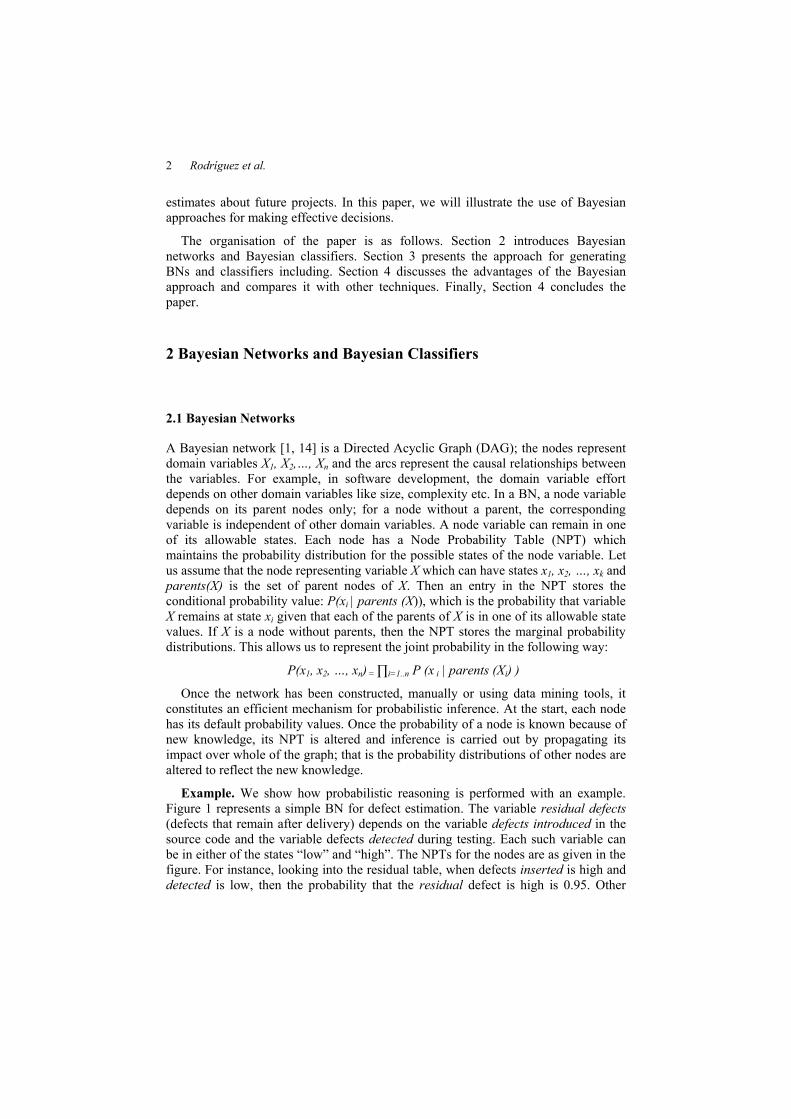
Example. We show how probabilistic reasoning is performed with an example.
Figure 1 represents a simple BN for defect estimation. The variable residual defects
(defects that remain after delivery) depends on the variable defects introduced in the
source code and the variable defects detected during testing. Each such variable can
be in either of the states “low” and “high”. The NPTs for the nodes are as given in the
figure. For instance, looking into the residual table, when defects inserted is high and
detected is low, then the probability that the residual defect is high is 0.95. Other
Bayesian Networks and Classifiers in Project Management 3
entries in the NPTs can be similarly explained. Note that the node defects inserted has
no parents; so, its NPT stores only the marginal probabilities.
Fig. 1. Example of BN for Estimates of Residual Defects
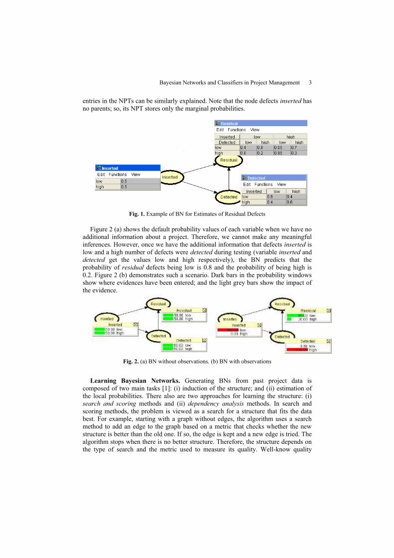
Figure 2 (a) shows the default probability values of each variable when we have no
additional information about a project. Therefore, we cannot make any meaningful
inferences. However, once we have the additional information that defects inserted is
low and a high number of defects were detected during testing (variable inserted and
detected get the values low and high respectively), the BN predicts that the
probability of residual defects being low is 0.8 and the probability of being high is
0.2. Figure 2 (b) demonstrates such a scenario. Dark bars in the probability windows
show where evidences have been entered; and the light grey bars show the impact of
the evidence.
Fig. 2. (a) BN without observations. (b) BN with observations
Learning Bayesian Networks. Generating BNs from past project data is
composed of two main tasks [1]: (i) induction of the structure; and (ii) estimation of
the local probabilities. There also are two approaches for learning the structure: (i)
search and scoring methods and (ii) dependency analysis methods. In search and
scoring methods, the problem is viewed as a search for a structure that fits the data
best. For example, starting with a graph without edges, the algorithm uses a search
method to add an edge to the graph based on a metric that checks whether the new
structure is better than the old one. If so, the edge is kept and a new edge is tried. The
algorithm stops when there is no better structure. Therefore, the structure depends on
the type of search and the metric used to measure its quality. Well-know quality

4 Rodríguez et al.
measure include the HGC (Heckerman-Geiger-Chickering), SB (Standard Bayes) and
LC (Local Criterion) measurement [12]. This problem is known to be NP-complete
[5], therefore, many of the methods use heuristics to reduce the search space such as
node ordering as an input. Search and score algorithms include: Chow and Liu [4], K2
[6] etc. Dependency analysis methods try to find dependencies from the data which in
turn are used to infer the structure. Dependency relationships are measured using
conditional independency tests [3].
2.2 BN Classifiers
Many SE problems like cost estimation and forecasting can be viewed as
classification problems. A classifier resembles a function in the sense that it attaches a
value (or a range or a description) to a set of attribute values. A classification function
will produce a set of descriptions based on the characteristics of the instances for each
attribute. Such class descriptions are the output of the classifier’s function. A BN
classifier assigns a set of attributes A1, A2,... An to a class description C such that
P(C | A1, A2,..., An,), that is the probability of the class description value given the
attribute instances, is maximal. Afterwards the classifier is used to classify a new
dataset. All BNs (usually called general BNs) can be used for classification where one
of the variables is selected as a class variable, and the remaining variables as attribute
variables. However, as commented previously, learning the structure of general BNs
is NP-complete [5] and more fixed structures have been applied to facilitate the
creation of the network. Such simpler approaches include:
Naïve Bayes [8] is the simplest Bayesian classifier to use and can be represented as
a BN with the class node as the parent of all other nodes and no edges between
attribute nodes, i.e., it assumes that all attributes are independent of one another,
which is violated in practice for most problems domains. Despite its simplicity, this
classifier shows good results and can even outperform more general structures.
TAN (Tree Augmented Naïve) augments the naïve Bayes structure with
dependencies among attributes having connections following a tree structure
(ignoring the output or class node). This classifier overcomes the assumption of
conditional independence between attributes. It was proposed by Friedman et al. [11].
FAN (Forest Augmented Naïve Bayes classifier) relaxes the tree structure of TAN
classifiers allowing some of the branches to be missing. Therefore, there will be a
number of a smaller trees spanning groups of nodes.
3 Effort Estimation using BNs and BN classifiers
In this section, we will show how data mining techniques and BNs can help acquiring
knowledge about the SE process of an organisation. The computational techniques
and tools designed to extract of useful knowledge from data by generalisation are
called machine learning, data mining or Knowledge Discovery in Databases (KDD)
[9]. Typical process steps include:

Bayesian Networks and Classifiers in Project Management 5
Data preparation, selection and cleaning. Data is formatted in a way that tools
can manipulate it and there may be missing and noisy data in the raw dataset.
Data mining. It is in this step when the automated extraction of knowledge from
the data is carried out.
Proper interpretation of the results, including the use of visualisation techniques.
Assimilation of the results.
We will illustrate this process using the dataset provided by Maxwell [17].
Construction of BNs involve a lot of intellectual activities in the sense of identifying
the variables and relationships between them. Therefore, expert guidance along with
information from past project data, if available, can be used in the generation process.
The Dataset. The dataset is composed of 63 applications from a bank. An excerpt
of the variables is described in Table 1. For further information refer to [17].
Table 1. Variable description
Variable Description
size Function points measured using the Experience method
effort Work carried out by the supplier from specification until delivery, (in hours)
duration Duration of project from specification until delivery, measured in months
source In-house or outsourced
… …
t01 to t15 Productivity factors such as requirements quality, use of methods etc.
3.1 Data pre-processing
In order to create a BNs and classifiers from data, datasets need to be pre-processed,
i.e., formatted, adapted and transformed for the learning algorithm. Typically, this
process consists of formatting the dataset, selecting variables, removing outliers,
normalizing data, discretising data, dealing with missing values, etc.
In our case, the Maxwell’s dataset was already formatted; before subjecting it to
data mining, we performed some minor editing. The variable syear, lan1 ,lan2, lan3
and lan4 were removed as we considered them irrelevant for our analysis. Such
editing also eliminated all the missing values. It was, however, necessary to discretise
all continuous variables as BN tools we used only worked with discrete data.
Discretisation consists of replacing a continuous variable with a finite set of intervals.
To do so, we need to decide whether a variable is continuous, the number of intervals
and the discretisation method. We decided to divide all three continuous variables into
10 equal range bins. Naturally, we lost some information in the process.
3.2 Model Construction
After data preparation, learning algorithms can be used for constructing BNs and BN
classifiers. This process consists of learning the network structure and generating the
node probability tables. The construction of naïve Bayes is trivial as the structure is
already fixed. The other Bayesian network structures such TAN, FAN and general
6 Rodríguez et al.
BNs need to find an appropriate structure out of many possible ones. In order to learn
the structure of the general BN, we may need to apply domain knowledge both before
and after the execution of the learning process. For example, we needed to edit the
network to add and remove arcs as it was impossible to do this from the data; this we
did based on the domain knowledge that we acquired from dataset analysis and from
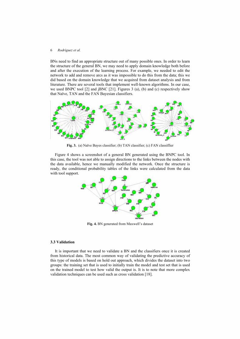
literature. There are several tools that implement well-known algorithms. In our case,
we used BNPC tool [2] and jBNC [21]. Figures 3 (a), (b) and (c) respectively show
that Naïve, TAN and the FAN Bayesian classifiers.
Fig. 3. (a) Naïve Bayes classifier; (b) TAN classifier; (c) FAN classiffier
Figure 4 shows a screenshot of a general BN generated using the BNPC tool. In
this case, the tool was not able to assign directions to the links between the nodes with
the data available, hence we manually modified the network. Once the structure is
ready, the conditional probability tables of the links were calculated from the data
with tool support.
Fig. 4. BN generated from Maxwell’s dataset
3.3 Validation
It is important that we need to validate a BN and the classifiers once it is created
from historical data. The most common way of validating the predictive accuracy of
this type of models is based on hold out approach, which divides the dataset into two
groups: the training set that is used to initially train the model and test set that is used
on the trained model to test how valid the output is. It is to note that more complex
validation techniques can be used such as cross validation [18].
Bayesian Networks and Classifiers in Project Management 7
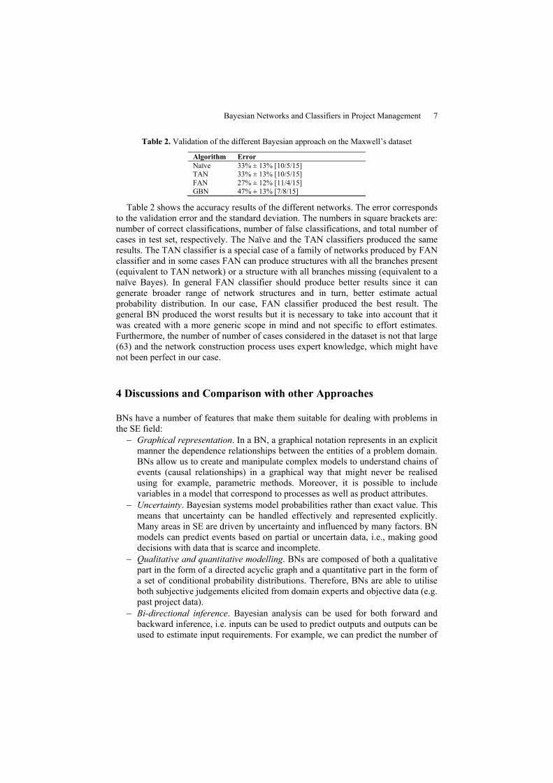
Table 2. Validation of the different Bayesian approach on the Maxwell’s dataset
Algorithm Error
Naïve 33% ± 13% [10/5/15]
TAN 33% ± 13% [10/5/15]
FAN 27% ± 12% [11/4/15]
GBN 47% ± 13% [7/8/15]
Table 2 shows the accuracy results of the different networks. The error corresponds
to the validation error and the standard deviation. The numbers in square brackets are:
number of correct classifications, number of false classifications, and total number of
cases in test set, respectively. The Naïve and the TAN classifiers produced the same
results. The TAN classifier is a special case of a family of networks produced by FAN
classifier and in some cases FAN can produce structures with all the branches present
(equivalent to TAN network) or a structure with all branches missing (equivalent to a
naïve Bayes). In general FAN classifier should produce better results since it can
generate broader range of network structures and in turn, better estimate actual
probability distribution. In our case, FAN classifier produced the best result. The
general BN produced the worst results but it is necessary to take into account that it
was created with a more generic scope in mind and not specific to effort estimates.
Furthermore, the number of number of cases considered in the dataset is not that large
(63) and the network construction process uses expert knowledge, which might have
not been perfect in our case.
4 Discussions and Comparison with other Approaches
BNs have a number of features that make them suitable for dealing with problems in
the SE field:
Graphical representation. In a BN, a graphical notation represents in an explicit
manner the dependence relationships between the entities of a problem domain.
BNs allow us to create and manipulate complex models to understand chains of
events (causal relationships) in a graphical way that might never be realised
using for example, parametric methods. Moreover, it is possible to include
variables in a model that correspond to processes as well as product attributes.
Uncertainty. Bayesian systems model probabilities rather than exact value. This
means that uncertainty can be handled effectively and represented explicitly.
Many areas in SE are driven by uncertainty and influenced by many factors. BN
models can predict events based on partial or uncertain data, i.e., making good
decisions with data that is scarce and incomplete.
Qualitative and quantitative modelling. BNs are composed of both a qualitative
part in the form of a directed acyclic graph and a quantitative part in the form of
a set of conditional probability distributions. Therefore, BNs are able to utilise
both subjective judgements elicited from domain experts and objective data (e.g.
past project data).
Bi-directional inference. Bayesian analysis can be used for both forward and
backward inference, i.e. inputs can be used to predict outputs and outputs can be
used to estimate input requirements. For example, we can predict the number of

8 Rodríguez et al.
residual defects of the final product based on the information about testing
effort, complexity, etc. Furthermore, given an approximate value of residual
defects the BN will provide us with a combination of allowable values for the
complexity, testing effort etc. which could satisfy the no. of residual defects.
Confidence Values. The output of BNs and classifiers are probability
distributions for each variable instead of a single value, that is, they associate a
probability with each prediction. This can be used as a measure of confidence in
the result, which is essential if the model is going to be used for decision
support. For example, if the confidence of a prediction is below certain
threshold the output for a Bayesian classifier could be ‘not known’.
There is to note that Bayesian classifiers are just one approach to classification and
there are many types of classifiers such as decision trees which output explicit sets of
rules describing each class, neural networks which create mathematical functions to
calculate the class, genetic algorithms etc. We now briefly summarise and compare
the Bayesian approach with the two most alternative approaches, rule based systems
and neural networks, used in software engineering.
Rule-based Systems vs. BN. A rule-based system [20] consists of a library of
rules of the form: if (assertion) then action. Such rules are used to elicit information
or to take appropriate actions when specific knowledge becomes available. The main
difference between BNs and rule based systems is that rule based systems model
experts’ way of reasoning while BNs model dependencies in the domain. Rules reflect
a way to reason about the relationships within the domain and because of their
simplicity, they are mainly appropriate for deterministic problems, which is not
usually the case in software engineering. For example, Kitchenham and Linkman [16]
state that estimates are a probabilistic assessment of a future condition and that is the
main reason why managers do not obtain good estimates. Another difference is that
the propagation of probabilities in BNs uses a global perspective in the sense that any
node in a BN can receive evidences, which are propagated in both directions of the
edges. In addition, simultaneous evidences do not affect the inference algorithm.
Neural Networks (NN) vs. BN. NN [19] can be used for classification and its
architecture consists of an input, an output and possibly several hidden layers in
between them; except for the output layer, nodes in a layer are connected to nodes in
the succeeding layer. In software engineering, the input layer may be comprised of
attributes such as lines of code, development time etc. and the output nodes could
represent attributes such as effort and cost. NNs are trained with past project data
adjusting weights connecting the layers, so that when a new project arrives, NNs can
estimate the new project attributes according to previous patterns. A difference is that
NNs cannot handle uncertainty and offer a black-box view in the sense that they do
not provide information about how the results are reached; however, all nodes in a BN
and their probability tables provide information about the domain and can be
interpreted. Another disadvantage of NN compared to BNs is that expert knowledge
cannot be incorporated into a NN, i.e., BN can be constructed using expert
knowledge, past data or a combination of both, while in NNs it is only possible
through training with past project data.
Bayesian Networks and Classifiers in Project Management 9
It is to note that Bayesian networks are statistical methods and therefore, the
structures presented here make assumptions about the form and structure of the
classifier. Depending on whether such assumptions are correct, the classifier will
perform well. Another drawback is that the data must be as clean as possible as noisy
data can significantly affect the outcome and several trials may be necessary to obtain
the right model. Further research is necessary to analyse the influence of discretisation
and the different number of quality measures used for creating TAN and FAN
classifiers. Finally, it is necessary to analyse how the number of data projects stored
influences the learning and posterior accuracy problem. Kirsopp and Shepperd [15]
have investigated problems with the hold-out approach concluding that using small
datasets can lead to almost random results.
5 Conclusions and Future Work
In this paper, we presented Bayesian networks and classifiers and discussed how they
could be used in the estimation and prediction problems in software engineering. In
specific, we presented four types of Bayesian classifiers and discussed their
similarities and differences. We also constructed instances of these classifiers from an
example dataset through semi-automatic procedures. However, our dataset size was
small, and therefore it could not effectively illustrate the merits of one over another.
This needs further investigation with large datasets. Effective construction of
classifiers is an intellectual task, and current tools are not adequate to address this
issue. More research is needed to produce classifiers with greater accuracy. We also
presented a comparative analysis of BNs, rule based systems and neural networks.
Our future work includes further research into how different Bayesian approaches
including its extensions such as influence diagrams and dynamic Bayesian networks
can be applied to software engineering. It includes how to integrate the different
Bayesian approaches into the development process and handle all kind of data
generated by processes and products. It will potentially make easier for the project
manager to access the vital software metrics data and perform probabilistic
assessments using a custom interface.
Acknowledgements. The research was supported by the Spanish Research Agency
CICYT- TIC1143-C03-01 and The University of Reading. Thanks are also to the
anonymous reviewers.
References
[1] E. Castillo, J. M. Gutiérrez and A. S. Hadi, Expert Systems and Probabilistic Network
Models. Springer-Verlag, 1997.
[2] J. Cheng, "Belief Network (BN) Power Constructor", 2001.
[3] J. Cheng, D. A. Bell and W. Liu, "Learning Belief Networks from Data: an
Information Theory Based Approach," 6th ACM International Conference on
Information and Knowledge Management, 1997.
10 Rodríguez et al.
[4] C. K. Chow and C. N. Liu, "Approximating discrete probability distributions with
dependence trees," IEEE Transactions on Information Theory, vol. 14462-467, 1968.
[5] G. F. Cooper, "The computational complexity of probabilistic inference using belief
networks," Artifcial Intelligence, vol. 42393-405, 1990.
[6] G. F. Cooper and E. Herskovits, "A Bayesian Method for the Induction of
Probabilistic Networks from Data," Machine Learning, vol. 9309-347, 1992.
[7] A. K. Delic, F. Mazzanti and L. Strigini, "Formalizing a Software Safety Case via
Belief Networks," Center for Software Reliability, City University, London, U.K.,
Technical report 1995.
[8] R. O. Duda and P. E. Hart, Pattern Classification and Scene Analysis. John Wiley
Sons, 1973.
[9] U. Fayyad, G. Piatetsky-Shapiro and P. Smyth, "The KDD Process for Extracting
Useful Knowledge From Volumes of Data", in Communications of the ACM, vol. 39,
1996, pp. 27-34.
[10] N. E. Fenton and M. Neil, "Software Metrics: Successes, Failures and New
Directions," Journal of Systems and Software, vol. 47, no. 2-3, pp. 149-157, 1999.
[11] J. Friedman, D. Geiger and M. Goldszmidt, "Bayesian Networks Classifiers,"
Machine Learning, vol. 29131-163, 1997.
[12] D. E. Heckerman, D. Geiger and D. Chickering, "Learning Bayesian Networks: The
Combination of Knowledge and Statistical Data," Machine Learning, vol. 20197-243,
1995.
[13] D. E. Heckerman, E. H. Mamdani and M. P. Wellman, "Real-World Applications of
Bayesian Networks", in Communications of the ACM, vol. 39, 1995, pp. 24-26.
[14] F. V. Jensen, An Introduction to Bayesian Networks. UCL Press, 1996.
[15] C. Kirsopp and M. Shepperd, "Making Inferences with Small number of Traning
Sets," IEE Procedings of Software Engineering, vol. 149, no. 5, pp. 123-130, 2002.
[16] B. A. Kitchenham and S. G. Linkman, "Estimates, Uncertainty, and Risk", in IEEE
Software, vol. 14, 1997, pp. 69-74.
[17] K. Maxwell, Applied Statistics for Software Managers. Prentice Hall PTR, 2002.
[18] T. M. Mitchell, Machine Learning. McGraw-Hill, 1997.
[19] P. Picton, Neural networks. Palgrave, 2000.
[20] S. J. Russell and P. Norvig, Artificial intelligence : a modern approach, 2nd ed.
Prentice Hall/Pearson Education, 2003.
[21] D. Sacha, "jBNC - Bayesian Network Classifier Toolkit in Java":
http://jbnc.sourceforge.net/, 2003.
[22] D. A. Wooff, M. Goldstein and F. P. A. Coolen, "Bayesian Graphical Models for
Software Testing," IEEE Transactions on Software Engineering, vol. 28, no. 5, pp.
510-525, 2002.
[23] H. Ziv and D. J. Richardson, "Constructing Bayesian-network Models of Software
Testing and Maintenance Uncertainties," Software maintenance, Bari; Italy, 1997, pp.
100-113.
Recommended


