Bouncing on Titan: Motion of the Huygens Probe inthe Seconds After Landing

Stefan E. Schrodera, Erich Karkoschkab, Ralph D. Lorenzc

aMax-Planck-Institut fur Sonnensystemforschung, 37191 Katlenburg-Lindau, GermanybLunar and Planetary Laboratory, University of Arizona, Tucson, AZ 85721-0092, U.S.A.cApplied Physics Laboratory, Johns Hopkins University, Laurel, MD 20723-6099, U.S.A.

Abstract

While landing on Titan, several instruments onboard Huygens acquired mea-surements that indicate the probe did not immediately come to rest. Detailedknowledge of the probe’s motion can provide insight into the nature of Ti-tan’s surface. Combining accelerometer data from the Huygens AtmosphericStructure Instrument (HASI) and the Surface Science Package (SSP) with pho-tometry data from the Descent Imager/Spectral Radiometer (DISR) we developa quantitative model to describe motion of the probe, and its interaction withthe surface. The most likely scenario is the following. Upon impact, Huygenscreated a 12 cm deep hole in the surface of Titan. It bounced back, out of thehole onto the flat surface, after which it commenced a 30-40 cm long slide in thesouthward direction. The slide ended with the probe out of balance, tilted inthe direction of DISR by around 10◦. The probe then wobbled back and forthfive times in the north-south direction, during which it probably encountered a1-2 cm sized pebble. The SSP provides evidence for movement up to 10 s afterimpact. This scenario puts the following constraints on the physical propertiesof the surface. For the slide over the surface we determine a friction coefficientof 0.4. While this value is not necessarily representative for the surface itselfdue to the presence of protruding structures on the bottom of the probe, thedynamics appear to be consistent with a surface consistency of damp sand. Ad-ditionally, we find that spectral changes observed in the first four seconds afterlanding are consistent with a transient dust cloud, created by the impact of theturbulent wake behind the probe on the surface. The optical properties of thedust particles are consistent with those of Titan aerosols from Tomasko et al.(P&SS 56, 669). We suggest that the surface at the landing site was covered bya dust layer, possibly the 7 mm layer of fluffy material identified by Atkinson etal. (Icarus 210, 843). The presence of a dust layer contrasts with the dampnessmeasured just centimeters below the surface, and suggests a recent spell of dryweather at the landing site.

Keywords: Titan, Titan surfacePACS: 96.12.Kz, 96.30.nd

Preprint submitted to Elsevier March 13, 2014

1. Introduction

The Huygens probe entered Titan’s atmosphere on January 14, 2005 andlanded on its surface after a 2.5 hour descent1. Images obtained by the De-scent Imager/Spectral Radiometer (DISR) revealed the landing site to be aflood plain strewn with rounded, decimeter-sized pebbles of unknown composi-tion (Tomasko et al., 2005; Karkoschka et al., 2007). The surface itself appearsfine-grained, damp, and relatively soft (Zarnecki et al., 2005; Niemann et al.,2005; Lorenz et al., 2006; Karkoschka et al., 2007), and may be covered by a7 mm thick fluffy layer (Atkinson et al., 2010). The motion of Huygens dur-ing atmospheric entry and descent has been studied well (Bird et al., 2005;Karkoschka et al., 2007; Lorenz et al., 2007), but its motion during and directlyfollowing landing has not. In the last phase of the descent a stabilizer parachuterestricted the vertical speed to 4.5 m s−1, ensuring a relatively soft landing. Thehorizontal speed was then only around 1 m s−1. It is clear that, upon impact,the 200 kg probe could not immediately have come to rest. Indeed, evidencefor continued motion exists. Schroder (2007) noticed that DISR measurementswere variable for several seconds after impact, and suspected that motion and/ordust between the detector and the surface had been responsible. Bettanini et al.(2008) analyzed Huygens Atmospheric Structure Instrument (HASI) accelerom-eter data, and proposed that the probe bounced back from the surface for 0.4 swith a horizontal speed of about 1 m s−1. The data indicated motion for afew more seconds after the bounce phase, which was not modeled. On the longterm Huygens seems to have been very stable. In the remaining 70 minutes thatCassini was visible over the horizon it may have tilted very slowly, at a rate onthe order of 0.1◦ per hour (Zarnecki et al., 2005; Karkoschka et al., 2007).

The goal of this paper is to develop a scenario for the events right afterlanding and to find a quantitative description for Huygens’ motion. We hope ourmodel not only fits the available data, but also offers insight into the physicalproperties of the surface. While the main focus is on the analysis of DISRdata, we can only obtain a complete picture when we include data from otherinstruments. A variety of instruments onboard Huygens were active aroundimpact. These can be roughly divided into two groups: accelerometers andphoto/spectrometers. Accelerometers were part of HASI, the Surface SciencePackage (SSP), and the Radial Accelerometer Sensor Unit (RASU), whereasseveral photo- and spectrometers were included in DISR. The sparse data maynot able to constrain all model parameters, and the solution may not be unique.Nevertheless, a quantitative model may allow a better understanding of Titan’ssurface near the landing site and of the dynamical interaction between the probeand surface. In addition, we look back at a drop test performed in Sweden witha Huygens model before launch, and assess whether it offers any clues to what

1Strictly speaking, Huygens impacted onto the surface. Post-impact survival of the probewas not a design driver, and the mission would have been considered a success even if nofurther contact had been made. Fortunately, the impact turned out to be a soft landing, sowe use the words “impact” and “landing” interchangeably.

2

happened on Titan.This paper is divided into two sections. The first describes our analysis

of the various data sets. The second describes the model we developed for theprobe motion in the seconds after landing. We end our paper with a summary ofour findings and discuss their implications for the physical properties of Titan’ssurface at the landing site. We have created several movies based on our motionmodel to visualize the events around landing. These, and a data file with thefull model results are provided as online supplementary material.

2. Data Analysis

The data described in this section were mostly acquired by instrumentslocated on the Huygens instrument platform inside the probe. We frequentlyrefer to instruments by their acronym, listed in Table 1. Their location onthe platform is shown in Fig. 1. This figure also defines the Huygens-centeredcoordinate system, in terms of which many of the data are discussed. The threeaxes are the X, Y , and Z-axis. The positive X-axis points up in the direction ofthe parachute, positive Z points toward DISR, and positive Y points 90◦ to theright of DISR. We use “mission time”, where impact is at mission time 8869.8 s.For exposures, the times quoted are mid-exposure.

2.1. Descent Imager/Spectral Radiometer (DISR)

The Descent Imager / Spectral Radiometer (DISR) was mounted on theHuygens instrument platform aligned with the Z-axis (Fig. 1). It carried im-agers, spectrometers, and photometers to measure photometric properties ofthe atmosphere and surface (Tomasko et al., 2002). In addition, DISR had aSurface Science Lamp (SSL), which was switched on before landing and stayedon. Several instruments recorded the spot on the surface illuminated by thelamp, in particular the Downward-Looking Visible Spectrometer (DLVS) andthe Downward-Looking Violet photometer (DLV). The Medium Resolution Im-ager (MRI) also probed the lamp spot, but images were not taken around land-ing. However, one CCD column (#49) was read out that probed the edge of theMRI image close to the lamp spot. The intensity distribution of the lamp spotcan be approximated by a Gaussian, with a FWHM of 3.5◦ (in the zenith-nadirdirection). It is centered on nadir angle 20.5◦.

Exposures of the DLV, DLVS, and column 49 were taken simultaneouslyabout once per second around landing until 50 s past impact, when DISRswitched to a different operation mode. These three data sets were transmittedto the Cassini spacecraft through two channels (A and B), but Cassini recordedonly in one channel (B) (Lebreton et al., 2005). Thus, the available data aresomewhat randomly spaced, and typically only data of one or two of the three in-struments exist for any specific time. An overview of the data acquired is shownin Fig. 2. Calibration of the DLV and DLVS was described by Karkoschka et al.(2012), and calibration of the data for column 49 was described by Schroder(2007). Below, we review the most important aspects for each instrument.

3

2.1.1. Downward-Looking Violet Photometer (DLV)

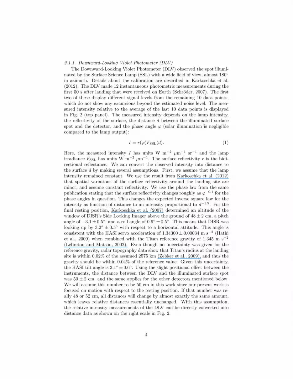
The Downward-Looking Violet Photometer (DLV) observed the spot illumi-nated by the Surface Science Lamp (SSL) with a wide field of view, almost 180◦

in azimuth. Details about the calibration are described in Karkoschka et al.(2012). The DLV made 12 instantaneous photometric measurements during thefirst 50 s after landing that were received on Earth (Schroder, 2007). The firsttwo of these display different signal levels from the remaining 10 data points,which do not show any excursions beyond the estimated noise level. The mea-sured intensity relative to the average of the last 10 data points is displayedin Fig. 2 (top panel). The measured intensity depends on the lamp intensity,the reflectivity of the surface, the distance d between the illuminated surfacespot and the detector, and the phase angle ϕ (solar illumination is negligiblecompared to the lamp output):

I = r(ϕ)FSSL(d). (1)

Here, the measured intensity I has units W m−2 µm−1 sr−1 and the lampirradiance FSSL has units W m−2 µm−1. The surface reflectivity r is the bidi-rectional reflectance. We can convert the observed intensity into distance tothe surface d by making several assumptions. First, we assume that the lampintensity remained constant. We use the result from Karkoschka et al. (2012)that spatial variations of the surface reflectivity around the landing site areminor, and assume constant reflectivity. We use the phase law from the samepublication stating that the surface reflectivity changes roughly as ϕ−0.1 for thephase angles in question. This changes the expected inverse square law for theintensity as function of distance to an intensity proportional to d−1.9. For thefinal resting position, Karkoschka et al. (2007) determined an altitude of thewindow of DISR’s Side Looking Imager above the ground of 48 ± 2 cm, a pitchangle of −3.1± 0.5◦, and a roll angle of 0.9◦± 0.5◦. This means that DISR waslooking up by 3.2◦ ± 0.5◦ with respect to a horizontal attitude. This angle isconsistent with the HASI servo acceleration of 1.34300 ± 0.00034 m s−2 (Hathiet al., 2009) when combined with the Titan reference gravity of 1.345 m s−2

(Lebreton and Matson, 2002). Even though no uncertainty was given for thereference gravity, radar topography data show that Titan’s radius at the landingsite is within 0.02% of the assumed 2575 km (Zebker et al., 2009), and thus thegravity should be within 0.04% of the reference value. Given this uncertainty,the HASI tilt angle is 3.1◦± 0.6◦. Using the slight positional offset between theinstruments, the distance between the DLV and the illuminated surface spotwas 50 ± 2 cm, and the same applies for the other detectors mentioned below.We will assume this number to be 50 cm in this work since our present work isfocused on motion with respect to the resting position. If that number was re-ally 48 or 52 cm, all distances will change by almost exactly the same amount,which leaves relative distances essentially unchanged. With this assumption,the relative intensity measurements of the DLV can be directly converted intodistance data as shown on the right scale in Fig. 2.

4

2.1.2. Column 49

Light for DISR’s visible spectrometers was recorded on the same CCD aslight for the imagers, but at levels some 100 times fainter. DISR had no shutters.Thus, when spectra were acquired the CCD got flooded with light from theimagers, and the part of the CCD where spectra were recorded received somescattered light. In order to account for this, data in column number 49 wererecorded because this column is located between the parts of the CCD recordingimages and spectra. Fig. 3 displays an image recorded by the Medium ResolutionImager (MRI) after landing. The bright spot on the surface at bottom right isoverexposed due to the strong illumination from the lamp. To the right of theMRI image on the CCD we find column 49, with rows 1-200 counted from thetop down (Fig. 3). Column 49 registers scattered light, and as such measuresthe brightness of the image near its right edge. Row 200 received almost 100times as much light as row 1 (Fig. 4, top panel). This is due to the fact thatthe reflector of the lamp focused light very strongly onto a relatively small spot,leaving the illumination further away fainter by several orders of magnitude.

During the first 50 s after landing, 17 exposures of column 49 were recorded.The exposures acquired around the time of landing exhibit intriguing variability(Schroder, 2007). The first of these was 1.36 s long and started already beforelanding, but ended after. Starting from the third exposure, all have essentiallyconstant signal within the noise level. Thus, we averaged these 15 exposures andthen normalized all data with respect to this average. We display smoothed,relative intensity curves in the bottom panel of Fig. 4. Even with the smooth-ing, the data are still noisy on the left side of the figure where original datanumbers were low. Similar to the DLV, the intensity varies as d−1.9, with d thedistance between the lamp spot and the detector. However, the changing par-allax between the lamp and the detector causes an even larger variation, whichchanges the dependency to d−4.3 close to the lamp spot, around row 190. Asexplained in Karkoschka et al. (2012), our software can create model images foreach requested distance. As the distance to the surface decreases, the parallaxmoves the bright spot further to the right in the image causing a large intensityincrease at the high row numbers. We created model images for various dis-tances and found a good fit to the second exposure (dashed curve in Fig. 4) forthe probe rolled by 1◦ toward the DISR side (i.e. a pitch-angle increase of 1◦),corresponding to a distance decrease by 1.5 cm. The intensity at rows 1-120increases by 5% due to the d−1.9 dependence. At higher row numbers, close tothe lamp spot, the increase is larger due to the parallax shifting the lamp spot.Thus, we can convert the relative intensity measurements near row 190 (secondpanel in Fig. 2) into a distance scale, shown at the right side of Fig. 2.

The first (1.36 s long) exposure started at an altitude of 3.8 m when theillumination of column 49 was less than 2% of the illumination after landing.Even at mid exposure, the illumination was still less than 20%. The relativelysmall amount of illumination before landing can be estimated and subtractedfrom the data. This gives a measurement of the illumination for the part of theexposure that occurred after landing (open symbol in Fig. 2). Near row 190, the

5

illumination was twice as bright as in the final resting position, toward row 1almost three times as bright. During the first half second after landing, thedetector must have been much closer to the surface than at the final position.We tried to model the shape of the solid curve in the bottom panel of Fig. 4,but we were unsuccessful.

While we believe that the detector was closer to the surface than in the finalposition, the quantitative connection of the intensity and distance as suggestedin Fig. 2 (left and right scale) is probably not accurate for this exposure. Theintensity curve for the first exposure (solid curve in the top panel of Fig. 4) ismuch smoother than all others, which suggests major motion during the firsthalf second after landing. The other 16 curves have all matching features thatcorrelate with features seen in MRI images (Schroder, 2007). This implies thatthe horizontal motion of Huygens must have been quite small (<1 cm) from thetime of the second exposure, 4.0 s after impact.

2.1.3. Downward Looking Visual Spectrometer (DLVS)

The Downward Looking Visible Spectrometer (DLVS) recorded spectra con-taining 200 data points between 480 and 980 nm wavelength. During the first50 s after landing, the DLVS acquired 19 exposures (Schroder, 2007). Each ofthese yields two spectra of the surface left of the lamp spot, one 4◦ above theother (Fig. 3). In reality, the spectrum of a specific location along the slit wasnot perfectly aligned along columns on the CCD, but was angled and curved.Thus, for 600 nm wavelength, for example, the two probed locations correspondto the solid black rectangles in Fig. 3, while for 950 nm wavelength they corre-spond to the dotted rectangles. Using exposures acquired in the laboratory andon Titan, Karkoschka et al. (2012) showed that the 400 data points for eachpair of spectra could be converted into 202 parameters, 200 of which correspondto a spectrum for the peak intensity along the slit. It was assumed that theshape of the spectrum does not change along the slit, based on spectra with 10spatial resolution points along the slit taken minutes after landing. From theseexposures it was also concluded that the spatial variation near the lamp spotcan be approximated well by a Gaussian shape. The two remaining parametersthen represent the spatial variation along the slit: the nadir angle of the peakintensity, and the full width at half maximum (FWHM) of the Gaussian. Theunused 198 data points (400 minus 202) were used to check that the methodand assumption were valid.

The resulting spectra of the peak intensity along the slit are shown in Fig. 5for the first five exposures. They are normalized to the average of the remaining14 spectra since these were all identical within the noise level. Due to therelatively long exposure time, the first exposure (1.36 s long at 8871.41 s) ismostly saturated between 670 and 830 nm wavelength in both CCD columns(dotted line of bottom curve in Fig. 5, linear interpolation). The exposure timeof the next exposure (at 8872.78 s) was automatically decreased by the onboardsoftware, and the central wavelengths are only saturated in the column probingthe surface closest to the lamp spot. This spectrum was reconstructed usingthe fainter signal of the other column, but the result is obviously noisier at the

6

central wavelengths (Fig. 5, top curve). Subsequent spectra were all correctlyexposed.

The basic intensity variation with changing distance is d−1.9, as before. How-ever, in this case the parallax works the opposite way as for column 49. As thedistance decreases, the lamp spot moves to the right, away from the probed ar-eas. This changes the intensity faster than the basic dependence. For distancesaround 50 cm, the intensity actually increases as d2.2. Based on our modeling,the variable intensities measured during the first five exposures can be explainedwith variable distance to the surface, as shown in the central panel of Fig. 2.However, the model assumes that all spectra have the same shape, so the nor-malized spectra in Fig. 5 should all be flat and horizontal. This is not the case.The slope of the first three spectra taken after landing is steeper (redder) thanthat of later ones. In fact, the slope relaxes with a 1/e time constant of about0.7 s. We consider several possible explanations.

Perhaps spatial variations across Titan’s surface are responsible. Since ourprevious work suggests that the shapes of the visible spectra around the landingsite are all almost identical (Karkoschka et al., 2012), we conclude that this isvery unlikely. Then, the impact might have changed something in the instru-ment that came back to normal on the observed time scale. We consider thisunlikely too.

Dust between the surface and the detector could have caused absorption witha temporal color variability. Lorenz (1993) speculated that sand or dust couldbe lofted for some time and might be detectable optically with DISR. Atkinsonet al. (2010) concluded that a 7 mm thick layer of a very fluffy substance lieson top of the surface at the landing site. It is natural to assume that this layerconsists of settled aerosols. Huygens’ impact might have suspended this layerin a dust cloud, which must have disappeared on a time scale shorter than asecond. Since very small dust particles do not fall significantly within 0.7 s,they must have been carried away by the atmosphere. The wind speed at thesurface was probably less than 0.25 m s−1 (Lorenz, 2006), and possibly evenlower at DISR’s leeward side. If wind were responsible, the dust cloud wouldhave been sized less than 15 cm to be consistent with the observed time scale.This is not credible. However, there is a turbulent wake behind a descendingprobe that dumps onto the ground as a ring vortex (Lorenz, 1993; Eames andDalziel, 2000). The terminal velocity of sand-sized particles (0.2 mm diameter)at Titan is only 10 cm s−1 whereas the velocity of the probe at impact, andthus the characteristic velocity in the wake, is 5 m s−1. So, dust on the sur-face could form a small toroidal cloud with a length scale of about one proberadius and be advected radially outwards. The expected velocities are a littleless than the descent speed (around 1 m s−1), consistent with the DLVS sloperelaxation time. We model the spectra in Fig. 5 assuming a dust cloud with op-tical depth inversely proportional to wavelength, the same as found for aerosolsbelow 30 km altitude (Tomasko et al., 2008), and achieve an excellent fit. Thederived optical depths given in the figure (0.75 at 600 nm for the first exposure)are for absorption along the double path from the lamp to the ground and backto DLVS.

7

Alternatively, the impact could have caused the lamp to temporally darkenand decrease its color temperature. This hypothesis fits the data in Fig. 5just as well as the dust model (not shown). The best fit equilibrium SSL colortemperature is 2750 K. The color temperatures derived for the first three spectraafter landing are 240, 40, and 10 K lower than equilibrium, which corresponds toa regular exponential decay with a factor of 1/e every 0.7 s. However, the firstpost-landing SSL voltage and current measurement (at 8874.09 s) does not showa significant change of power consumption. If a change in color temperature wascaused by a very brief interruption of the power, then we cannot explain theslow return to the nominal color temperature. A typical light bulb like thatof the SSL should respond much faster to switching on and off. We consider achange in color temperature an unlikely explanation for the DLVS slope change,and we favor the dust hypothesis.

What remains to be explained are the features at the left edge for the firsttwo exposures (Fig. 5). Actually, the upturn of the curve shortward of 550 nmwavelength for the first exposure and the downturn for the second exposure areexpected. If the distance decreases, the parallax moves the lamp spot furtherto the right, which means that the observed area is illuminated by light raysfurther away from the lamp axis. These have less contribution from the gold-plated reflector of the lamp. Gold has almost constant reflectivity longwardof 550 nm but lower reflectivity toward the blue part of the spectrum. Thus,the stronger contribution from direct light increases the blue illumination, asobserved for the first exposure. The situation for the second exposure is justopposite.

The DLVS data provide us two other independent measures of the distanceto the surface. We return to the two remaining parameters mentioned at thebeginning of this section which describe the spatial variation of light along theslit: the width and nadir angle of the peak intensity. The width is estimated asthe FWHM of a fitted Gaussian. Due to parallax, if the distance decreases, thelamp spot moves to the right in Fig. 3, and the sampled region far away from thespot has a broad, shallow maximum. For larger distances, the sampled area isclose to the sharply peaked center of illumination. Between DLVS spectra takenbefore landing and those long after landing, the FWHM increases by 80%, justas expected from our modeling. Thus, we are confident that we can convertthe variation of FWHM recorded during the first exposures after landing intoparallax variations and thus distance variations (fourth panel of Fig. 2, rightscale). Because our model suggests that the inverse of the FWHM is almostlinearly related to the distance between the detector and the ground, we plotthe inverse of the FWHM on the left side of the fourth panel.

The nadir angle of the peak intensity can also be converted into a distance.The DLVS aperture is further away from the vertical axis of Huygens than thelamp. Thus, a changing distance has a small but measurable parallax effect inthe vertical direction. We measured this effect between spectra taken beforelanding and those taken long after landing and found it consistent with ourexpectation from our model. Thus, we can convert the measured shift in thelocation of the peak intensity into distance changes (Fig. 2, bottom panel, right

8

scale).

2.1.4. Combined DISR data

The data in Fig. 2 suggest that around mission time 8871.5 s, DISR wascloser to the surface by about 10 cm than in the resting position. One secondlater, all data suggest an increased distance with respect to the resting positionby about 4 cm. Another second later, the sign changed again to a distance about2 cm less than in the resting position. From this moment on, the data points ofFig. 2 do not suggest any consistent motion. The noise associated with the DLVdata is quite large, it is moderate for the DLVS peak location, and quite smallfor the remaining three parameters. The moderate disagreement between thedistance data for the exposures before 8874 s is mostly due to uncertainties in themodeling. For some of the parameters where parallax changes the distributionof light, we do not expect our model predicts variations more accurately than20%.

Considering that the noise is low for three parameters, in particular for theintensity and FWHM of the DLVS, we investigated whether we could detectany motion after 8874 s. In Fig. 6, we show these data points in the top andmiddle panels. In order to decrease the noise, we averaged data numbers acrossthe whole spectrum. The lower panel averages the distance estimates from boththe top and middle panels. All data points after 8878 s are consistent with theestimated noise level of 0.05 cm, but the first two data points are off by +0.3and −0.2 cm, respectively, which corresponds to 6σ and 4σ. Thus, we concludethat Huygens still moved until 8878 s. Afterwards, the data are consistent withno motion. There is a slight chance that Huygens still moved when the datapoint at 8879.4 s was taken, but that this exposure was done when Huygenswas half way between extremes. Thus, we cannot exclude motion during thatexposure, but if Huygens was still in motion, the amplitude was probably verysmall.

Our data constrain only one parameter: the distance between the detectorand the spot on Titan’s surface illuminated by the lamp. The other five pa-rameters describing the position and orientation of Huygens are unconstrained.Nevertheless, we can guess which type of motion occurred. During these ob-servations, in particular in the later stages, Huygens was most likely constantlyin contact with Titan’s surface. Then, our measurements of the changing dis-tance were due to the probe wobbling, changing the pitch angle in a dampedoscillation. The roll and azimuth angle could have changed too, which wouldnot be noticed in our data unless the variations were very large. Assumingthat Huygens remained in contact with a flat surface, we convert the distancemeasurements into pitch angles (bottom left scale in Figs. 6 and 7). The noisein our data corresponds to an uncertainty for variations in the pitch angle of0.03◦, or 2 arcminutes, which is a remarkably high precision.

The dust hypothesis is our preferred explanation for the slope changes ob-served for the DLVS spectra after impact. How would the presence of dust inthe optical path length have affected the other DISR measurements? Lorenz(1993) calculated a dust cloud was possible based on the expected properties of

9

the wake behind the probe. But the actual dynamics of the dust cloud are hardto predict. Dedicated computational fluid dynamics studies or scale model testswould be needed to identify the characteristic lengths and times of the turbu-lent dust cloud. By the time of first DLV exposure after landing, the dust wasalready quite subdued. The remaining dust should have absorbed some lamplight, but should also have scattered some lamp light in the backward direction.It is not clear which of these effects wins, so the DLV data cannot provide usany insight. For column 49 data, the exposure that started before landing maybe affected by the presence of dust, but it is hard to know how. For the nextexposure, the expected density of dust was already close to negligible. So, alsothe column 49 data are noncommittal. To minimize the effect of dust on theDLVS slope we use the data around 900 nm wavelength to quantify the DLVSintensity in Fig. 2. More dust increases the slope and decreases the intensity.This results in a lower inferred distance for the DLVS, a larger distance for theDLV, and no distance change for the other three measured parameters. Thus,averaged for all five parameters in Fig. 2, dust has a small effect on the distancescale, smaller than uncertainties from the modeling.

2.2. Huygens Atmospheric Structure Instrument (HASI)

The Huygens Atmospheric Structure Instrument (HASI) piezo-accelerometerswere mounted on the Huygens instrument platform near the probe center of mass(Fulchignoni et al., 2002) (Fig. 1). They recorded the acceleration in all threedirections of the Huygens XY Z-coordinate system, from 0.8 s before landing to5.3 s after landing (Bettanini et al., 2008). We retrieved the HASI data fromNASA’s Planetary Data System (Witasse et al., 2008). The data for the X-and Z-directions are plotted in Fig. 7 (top panel) as solid curves2. FollowingBettanini et al. (2008) we plot positive X-acceleration values when the vectoris pointed towards the negative X-direction (downward). In line with this con-vention, positive Z-accelerations point away from DISR. Bettanini et al. (2008)postulated the existence of a period of free fall right after impact, resulting froma bounce. The raw data have a bias value, which we determined by forcing theacceleration to be zero during this bounce phase. Our bias determination couldbe off by 0.5 data number (DN) for each curve, and the digitization for alldata points could also cause an error by 0.5 DN. Thus, our goal is to developa motion model that can fit the data within 1 DN, which is indicated by thevertical width of the gray areas in Fig. 7. Bettanini et al. (2008) integratedthe HASI data and reconstructed a horizontal motion of about 1 m s−1 in theZ-direction during the bounce phase, followed by a sliding, decelerating motion

2Note that there is uncertainty regarding the direction of the HASI Y -axis. Figure 1 inBettanini et al. (2008) shows the HASI axes aligned exactly with the Huygens XY Z-axes.On the other hand, the text reads “the sensing axes of the HASI accelerometers were allinstalled along the positive direction of the Huygens reference axes except for the piezo-Yaccelerometer, which faced the Y -direction”, which meaning is not clear. We were unable toobtain clarification on this issue. We assume that the accelerations as shown in Fig. 2 inBettanini et al. (2008) are those in the Huygens XY Z- frame.

10

on the surface. The primary impact at mission time 8869.8 s caused a maxi-mum vertical acceleration of 120 m s−2 (off-scale in Fig. 7), due to the probe’sdeceleration within 12 cm (Zarnecki et al., 2005). The authors considered twopossibilities; that (1) Huygens either created a hole and bounced out of it, orthat (2) it displaced a pebble on the surface and ceased vertical motion just atground level. We consider the second possibility unlikely. Our new result fromSec 2.1 is that Huygens could not have been perched on a pebble because DISRwas very close to the surface during the first half second after impact. Also,data from the penetrometer of the Surface Science Package (Atkinson et al.,2010) might be difficult to explain. Furthermore, the secondary impact afterthe bounce phase would have occurred with an impact speed of 0.27 m s−1, whilethe HASI X-acceleration spike at that time suggests a vertical speed change ofonly 0.05 m s−1. All these observations can be better explained with the firstpossibility, which we adopted for our motion model in Sec. 3. Thus, for therest of this work, we assume that Huygens made first contact with Titan at theground level, which implies that it was digging a hole of 12 cm depth.

After the primary impact, the probe had a zero-g phase for a duration of0.4 s, indicating a bounce with no surface contact (Bettanini et al., 2008). Sub-sequent X- and Z-accelerations had some significant variations for a few secondsuntil settling down. The Y -acceleration on the other hand was 70% near zero,10% at +1 DN, and 20% at −1 DN (1 DN corresponds to about 0.2 m s−2).These low signals indicate that most of the motion was in the X-Z plane (c.f.Sec. 2.5). By correlating the Y - and Z-data we determine an average motionvector of about 3◦ to the left of the Z-axis (Fig. 8). Using the azimuth of 193±5◦

(13◦ west of south) for the Z-axis of Huygens at rest from Karkoschka et al.(2007), the motion vector of Huygens was around azimuth 190◦, very close topointing south, consistent with SSP measurements (see Sec. 2.3).

After the bounce and slide phase, Huygens wobbled on the surface for severalseconds. This was already inferred from DISR data (Sec. 2.1.4), but the HASIdata allow us to model it in detail as a damped oscillation. This model, theparticulars of which are described in Sec. 3, is drawn in the top panel of Fig. 7.In the bottom panel, we see how the probe pitch angles derived from DISR datain Sec. 2.1.4 compare to the model predictions. Not all model parameters arederived from HASI data exclusively; the damping time constant of the oscillationis based on DISR observations because the HASI data do not extend beyond8875 s. The DISR-derived pitch angles provide an independent test for ourmotion model, and the good fit of the data in the bottom panel in Fig. 7 mayconvince the reader that it has passed the test.

2.3. Surface Science Package (SSP)

The Surface Science Package (SSP) was mounted on the instrument platformrotated by 30◦ with respect to the Huygens Y and Z-axes (Zarnecki et al., 2002)(Fig. 1). Continued motion after impact is also supported by data from SSPsensors (Zarnecki et al., 2005). One of these is a density sensor, a small floatcantilevered on a strain gauge, which fortuitously also functioned as a crudeaccelerometer (Lorenz et al., 2007). Sampling of this sensor was interrupted

11

shortly after landing while a packet of priority data was assembled in the in-strument (Leese et al., 2012), but the timed data (Fig. 9) shows motions orvibrations at least until mission time 8873.6 s (4 s after impact). The signal hasreturned to quiescent levels by 8880 s. This is suggestive of continued motion,even though the possibility that the sensor experienced relaxation cannot beexcluded. The others are two radially oriented tilt sensors, used to monitorthe descent (Lorenz et al., 2007). These tilt sensors measured the position ofa small slug of conductive fluid in a cylindrical vial, thus (in steady state) giv-ing an indication of the orientation relative to the gravity field. In a dynamicenvironment they indicate lateral accelerations.

The time stamps on the SSP tilt records as archived on the PDS are inerror (though may be corrected in due course). We used corrected timing ofthe tilt data by Leese and Hathi (private communication) to make it consistentwith that of the DISR and HASI data sets. We restrict the tilt angle rangein Fig. 10 to clearly show the subtle tilt variations recorded a few secondsafter impact, which appear to indicate that the probe performed a dampedoscillation or wobble. A maximum occurs near mission time 8874.2 s, with atotal tilt of about 10◦ relative to the stable position. This tilt corresponds toa Z-acceleration of +0.2 m s−2 (Titan’s gravity multiplied by sin 10◦), which isconsistent with the actual HASI reading within the quantization (Fig. 7). Ourmodel predicts a pitch angle of −1◦ relative to the stable position. This impliesthat about 90% of the tilt data during the wobble was due to the accelerationof the probe, and only 10% due to the tilt of the probe. Soon afterwards, HASIstopped recording. DISR recorded another two cycles of the wobble, while SSPcovered 3-4 more cycles. So, including the 1.5 cycles of wobble before 8874.2 s,we have evidence for five complete cycles of wobble. The second maximum ofthe fifth cycle, or the tenth maximum of the wobble, occurred near mission time8880 s with a tilt of 0.2◦ off the stable value, corresponding to a probe pitchangle +0.02◦ off the stable position.

The data from the two tilt sensors in Fig. 10 are strongly correlated afterimpact, indicating that the wobble motion was planar. The bottom panel inFig. 8 shows that this correlation corresponds to an average motion in a direction3◦ left of the Z-axis, exactly as determined from HASI data (top panel; seeSec. 2.2). This remarkable agreement is a testament to the high quality of thedata of both instruments.

2.4. Radial Accelerometer Sensor Unit (RASU)

The Huygens probe carried the Radial Accelerometer Sensor Unit (RASU)to measure the probe spin rate (Fig. 1 shows its location on the instrumentplatform). RASU data was telemetered at irregular intervals. These data, whichalso shed light on turbulent motions of the probe during descent (Lorenz et al.,2007), are archived on the PDS Atmospheres Node in the Huygens housekeepingdata directory3. The data around impact from one of the accelerometers are

3Data set ID is HK CDMS RASU D8005A.TAB

12

shown in Fig. 11. The first signs of impact are only evident after 8872 s, whichsuggests that RASU time is offset by about 2 s from mission time. The signaldoes not return to quiescent levels until 8879.5 s, suggesting a combination ofprobe motion and/or structural ringing persisting for at least 7 s after impact.

2.5. Automatic Gain Control (AGC)

The gain of the signal from Huygens received by Cassini, the Automatic GainControl (AGC), was measured at a frequency of 8 Hz. Before landing it varieddue to the spin of Huygens at a rate around 1 RPM (Karkoschka et al., 2007).After landing, it continued to vary for a few seconds due to probe motion. SinceCassini was located roughly in the direction of the Y -axis of Huygens, the mainpart of the motion in the X-Z plane would not have caused much variation.So, for a few seconds after landing, there must have been some spin around theX-axis, or the probe was rolling around the Z-axis, or both. Because we do notknow the exact orientation of the probe around landing, we cannot model thevariations of the AGC. Even if we could, we would not be able to distinguishbetween spinning and rolling. Based on the size of the AGC variations afterlanding compared to before, one can estimate that the spin after landing wason the order of 10◦, or that the rolling after landing was on the order of a fewdegrees. The roll angle at rest was 0.9◦ ± 0.5◦ according to Karkoschka et al.(2007). Thus, the real motion had a significant component out of the X-Zplane, but we do not have sufficient information to constrain it.

2.6. Huygens drop test

Since post-impact survival of Huygens was not considered a design driver forthe probe, there was no program of full-scale impact tests. However, some in-sights can be gleaned from a parachute system test with Special Model 2 (SM2)4,made in 1995 from a stratospheric balloon over Kiruna in Sweden (Jakel et al.,1996; Underwood, 1997; Lorenz, 2010). Demonstrating the heat shield sepa-ration and parachute deployment sequence at flight-like conditions, the SM2test used a large (non-flight) recovery parachute to accommodate Earth’s atmo-sphere and gravity, which reduced the impact speed to around 8 m s−1. Theimpact was recorded by onboard accelerometers (Fig. 12), which clearly showa structural or dynamic bounce about 0.2 s after impact (the vertical accelera-tion dropped to 5 m s−2 or 0.5g). Most relevant here, after impact the lateralaccelerometers showed acceleration variations on the order of 0.15 m s−2 for aduration of 4 s.

The test report documents the conditions under which the vehicle was recov-ered (Brouwer, 1995): “The snow at the landing site was probably 0.5-1 m thick.The descent module had landed on the fore dome and was dragged over about1m through the snow. The impression in the snow was about 20 to 30 cm deep.The recovery parachute was lying nicely in a straight line next to the descent

4SM2 is now the Huygens model most often seen at exhibitions, and is easily identified bythe transparent window on its upper surface used to film the parachute deployment.

13

module. On first sight hardly any damage was visible, except for bending of thespin vanes. Some flattening of the fore dome had occurred. At arrival it could beheard that the gyroscopes were still running.” An inspection of the photo in thereport indicates a smooth depression or skid mark about 0.5 m long (Fig. 12).Thus in many ways, the landing of the SM2 vehicle resembled the dynamics wehave reconstructed for the Huygens probe on Titan.

3. A Model for Huygens’ Motion

3.1. Model description

We have created a description of Huygens’ motion after impact that is con-sistent with both the HASI accelerometer and DISR photometry data sets. Itconsists of several phases: creation of a hole through impact, bounce out of thehole, slide over the surface, and wobble on the surface. We model the probe mo-tion from the bounce phase to its final resting position. The model is describedbelow, with details of the numerical integration provided in the next section.We use the following basic parameters for Huygens from Lebleu (2005): a massof 200.5 kg, centered about 30 cm above the bottom of the probe, a bottomforedome with a nadir radius of curvature of 1.215 m, and a moment of inertiaof 24.5 kg m2 for rotations around the Y -axis. The model is two-dimensional(horizontal and vertical) since the HASI data suggest that most of the motionoccurred in the X-Z plane.

We start our modeling with the assumption that the surface of Titan washorizontal and flat until Huygens created a 12 cm deep hole upon impact. Fromthe shape of the foredome we infer that this hole had a radius of 53 cm. Theprobe must have been approximately level at this time because of the smallnessof Y - and Z-accelerations during the impact phase. After bouncing out of thehole the probe slid over the surface, decelerating through friction. The initialphase of the slide is complicated, as the probe did not necessarily end the bouncephase with a purely horizontal motion at ground level. This led to a secondaryimpact, which is considered in our modeling. We assume a constant frictioncoefficient throughout the slide. Note that this is the total friction coefficient ofthe slide, which is not necessarily equal to the friction coefficient of the surface(see Sec. 3.4). The plateau of the HASI Z-acceleration between mission times8870.4 and 8871.6 s suggests that the slide lasted about 1.2 s. Integrating thisplateau value near −0.8 m s−2 over the slide time, or integrating all Z-dataafter the bounce phase, yields a speed near −1 m s−1 in both cases. Bettaniniet al. (2008) interpreted this as a horizontal impact speed of 1 m s−1, decreasingto zero after the slide. We refine this estimate by considering that the probewas probably tilted, which means that part of the Z-data reflects a componentof the gravity, and not a decelerated motion. A tilt is expected on basis of thefollowing argument. The friction force in the negative Z-direction acted on thebottom of the probe and thus caused a negative angular acceleration (αY ) ofthe probe around the Y -axis. The front end of the probe would have tilteddownward, which we define as a positive pitch angle (θ). Because of the shape

14

of the bottom of the probe, a positive pitch angle causes the contact point withthe surface to move ahead of the probe’s center of mass, which then causesa positive angular acceleration around the Y -axis. Both angular accelerationscancel each other for a pitch angle around 12◦. However, a 12◦ pitch anglecauses a −0.28 m s−2 component of the gravity vector in the Z-direction. Thus,the actual deceleration was somewhat less than the Z-plateau value. Also,the actual horizontal impact speed was somewhat less than 1 m s−1, and theequilibrium pitch angle was more like 9◦, consistent with our simulation results.

At the end of the slide, the friction force due to sliding suddenly droppedto zero, which caused a drop of the measured horizontal acceleration. In Fig. 7we see how the Z-acceleration rapidly returned to values near zero at missiontime 8871.8 s, which makes this the most likely time when the sliding motionstopped. As we have shown, the pitch angle was now positive and the probe outof balance. This is the start of the wobble phase. For a frictionless wobble, theperiod of this almost harmonic oscillation would have been 2.2 s, as calculatedfrom Huygens’ moment of inertia. In reality, the wobble was damped, and weassume an exponential decay of the amplitude. The Z-acceleration (Fig. 7,top panel) suggests such a decaying wobble, but the period seems to be closerto 1.9-2.0 s. The phasing of the five main DISR data points (bottom panel)is also more consistent with a period near 2.0 rather than 2.2 s. The periodis very sensitive to the shape of the surface. A slightly convex surface wouldincrease the period, a concave surface would decrease it. The period near 2.0 ssuggests that the surface where the probe came to rest was slightly concave,and we calculate a radius of curvature of 6.5 m. However, DISR post-landingimages show a very flat surface with an abundance of pebbles (Karkoschka et al.,2007). One of these sticking out of the surface by 1-2 cm could also have causethe decreased period of wobbling. Additional evidence for a pebble stuck underthe probe comes from the pitch angle of −3.1◦ ± 0.5◦ calculated for the stableposition, which implies a slope of 2.3◦±0.4◦ for a flat surface (Karkoschka et al.,2007). The time constant for the exponential decay of the wobble amplitude(i.e. the time for the amplitude to decrease by a factor of 1/e) is estimatedfrom the HASI Z-acceleration data to be 1.2-1.6 s. The longer time coverageof the DISR data suggests a time constant of 1.4-1.6 s in case the observationsroughly probed the peak amplitudes. Thus, we adopt a time constant of 1.5 s.This means that every successive peak amplitude is about half a large as theprevious one. In order to model the wobbling motion with decaying amplitude,we assume that the contact point, and thus the location of the force from theground, is not exactly at the point indicated by the ideal geometry but slightlyforward, and that the displacement is proportional to the wobbling speed. Thelast DISR observation that indicated a position off from the resting position wasrecorded 7.7 s after impact. At this time, the wobbling amplitude was small,with the pitch angle being only 0.1◦ off the stable value. SSP data indicatecontinued wobbling motion for another 2 s with even smaller amplitudes.

15

3.2. Numerical integrationOur two-dimensional numerical model has a total of six time-dependent vari-

ables: two for the location of the probe (X and Z), one for the pitch angle (θ),two for both speed components (vX and vZ), and one for the angular speedaround the Y -axis (ωY ). From these we compute the two acceleration compo-nents (aX and aZ) and the angular acceleration (αY ). The accelerations enableus to compute new values for each of the variables for the next time step ∆t,typically chosen as 1 or 2 ms. Model time t = 0 is defined at the start of thebounce phase, when Huygens was resting on the bottom of a 12 cm deep hole.For the subsequent bounce, the only force considered is Titan gravity acting onthe center of mass (small forces, such as wind resistance, are neglected). Oncethe probe reaches contact with the surface again, the two components of thesurface force are two unknown variables. We distinguish the force componentsparallel and perpendicular to the motion vector (F‖ and F⊥). These are solvedwith two equations. One equation comes from our assumption that the probestays constantly in contact with the surface. The other equation is different forsliding and wobbling motion. For the slide, the friction coefficient of the surface(µ) comes into play: F‖ = µF⊥. For the wobble, the speed is zero for the partof the foredome that is in contact with the surface.

We performed several numerical simulations in which we varied the initialvalues for the two components of the initial speed and the friction coefficient.For any assumed horizontal speed v0Z , the vertical speed v0X and the frictioncoefficient µ can be constrained well from the timing of the HASI accelerationdata (Fig. 7, top panel). If v0X is too small or too large, the bounce phase willlast too short or too long, respectively, compared to the observed 0.4 s duration.If µ is too small or too large, the change of the horizontal acceleration aZ fromnegative to positive values will occur too late or too early, respectively, comparedto the observed mission time of 8871.8 s. We estimate v0Z from the HASI aZdata, and find a best fit for v0Z = 0.8-0.9 m s−1. Our result is consistent with the1 m s−1 from Bettanini et al. (2008), who found this value by integrating aZ onthe assumption that the probe did not tilt. For speeds less than 0.6 m s−1, theprobe is not able to make it out of its hole during the bounce phase, or it onlyleaves the hole temporarily, but then rolls back into it. This is inconsistent withthe analysis by Karkoschka et al. (2007) indicating that the bottom of the probewas within about 2 cm of to ground level by the time the probe came to rest.Thus, our best guess for the initial horizontal speed is v0Z = 0.8±0.1 m s−1. Ourbest guess for the initial vertical speed is v0X = 0.56 m s−1. A slightly smalleror larger v0X will cause a shorter or longer bounce phase, respectively, than theobserved 0.4 s. Thus, v0X is better constrained than v0Z .

The distance covered during the slide over the surface is not well constrained.In the nominal model, the probe comes to rest 86 cm south of the impact point.The resting point is located at least 70 cm south of the impact point (or 17 cmsouth of the edge of the hole). The 12 cm hole the probe created by the impacthas a 53 cm horizontal radius (give or take a few cm due to the uncertaintyin depth). Thus the probe cannot end up less than 53 cm south of the impactpoint because otherwise it would have rolled back into the hole. For a distance

16

between 53 and 70 cm the probe would have gone to the edge of the impacthole during the first wobble back. This would have lengthened the time for thatwobble, which is not supported by the data in Fig. 7. For distances beyond110 cm south of the impact point, the model fit to the HASI acceleration is notsatisfactory. Thus, the slide distance is somewhere between 20 and 50 cm, witha nominal value of 33 cm. The probe slide is terminated by surface friction. Wecalculated the friction coefficient for the slide as the friction force divided bythe weight of the probe. We found reasonable fits for values between 0.3 and0.5, and adopt 0.4 ± 0.1.

Even though we started our modeling by assuming that the probe was ap-proximately level at the start of the bounce phase, the model fit improves whenwe allow for a non-zero pitch angle upon impact. This would not affect theshape of the hole, nor would it change the horizontal speed. However, it wouldmake the center of the hole, and thus the impact force, horizontally offset fromthe probe center of mass. This, in turn, would cause the probe to leave the holewith a non-zero angular speed. Our adopted model has an initial angular speedof ω0

Y = 0.15 s−1, but this value is not well constrained. Considering the changeof the vertical speed of ∆vX = 5.1 m s−1 and the geometry of the probe, thisω0Y value is obtained in case the center of mass is offset by 0.4 cm, corresponding

to a pitch angle at impact of −0.23◦. This value is well within the average tiltangle of 1.5◦ obtained for the descent at low altitudes (Karkoschka et al., 2007).A negative pitch angle is also consistent with negative Z-accelerations recordedbefore impact. Furthermore, as shown in Sec. 3.5, the independently inferredvertical wind speed profile would also make the parachute-probe system tilt tonegative pitch angles seconds before impact.

Figure 13 shows the four main phases around the time of landing. A movieshows the motion and the forces (supplementary material). At the bottomtwo panels of Fig. 13 and for two additional movies, we also considered cases ofhorizontal speeds of v0Z = 0.67 and 0.66 m s−1, instead of the adopted 0.80 m s−1,leaving all other parameters unchanged. In the case of v0Z = 0.67 m s−1, theprobe takes a very long time for its first wobble period, which is inconsistent withobservations. In the case of v0Z = 0.66 m s−1, the probe rolls back into its holeand ends up with a pitch angle θ = −29◦, very inconsistent with observations.

3.3. Rolling over a pebble

When comparing the predictions of our motion model with the HASI accel-erations in Fig. 7 (top panel) we note two major deviations, one between missiontimes 8871.5 and 8872.0 s, and the other between 8872.0 and 8872.8 s. First wefocus on the latter event.

Had Huygens rolled over a pebble, it would have left a clear signature in theacceleration data. The recorded vertical acceleration would suddenly jump wayabove Titan’s gravity, as the vertical speed changes to the positive value neededto climb the pebble. Then, during the roll over the pebble, the vertical speedwould drop to negative values, which decreases the recorded vertical accelerationto values below Titan’s gravity. Finally, when the ground is reached again, therecorded acceleration jumps for a short time above Titan’s gravity. In case the

17

probe stopped on top of the pebble and rolled back where it came from, therecorded accelerations would have been similar. Considering that rolling frictionslowed the probe down, the initial motion onto the pebble would have causedlarger accelerations, of shorter duration, compared to the exit from the pebble.There is one event in the HASI data that matches the expected accelerations forrolling over a pebble almost perfectly, between mission times 8872.0 and 8872.8 s.During this period, the rolling motion reverses according to our model. Weintegrated the offset between the observed acceleration and the modeled valuestwice, and we determined the two integration constants by setting the height ofthe probe to zero at the beginning and end of this period. Then, the height ofthe probe in the middle of this period comes out to 2 cm. Thus, the probe rolledover a pebble sticking 2 cm out of the ground. Since this took place when theprobe was tilted with a negative pitch angle, we find a similar signature withsame sign, but lower amplitude, in the Z-acceleration data. If Huygens rolledover a pebble during the first wobble back, one might expect it should have goneover the same pebble during the slide. Yet, the data suggest this was not thecase. Our expectation is only true if the motion was purely in the X-Z plane.Likely, some smaller motion also occurred in the Y -direction. Thus, Huygensprobably did not exactly trace back the track of the slide during its first wobbleback. This explains why it only encountered the pebble during the first wobbleback, but not during the slide.

Our motion model cannot reproduce the other major deviation, the X-accelerations between 8871.5 and 8872.0 s. All model runs create values nearTitan’s gravity while the data show only half that value. The only way to matchthese data is to start with a larger initial vertical speed for the bounce whichputs the probe about 50 cm above ground for the slide and wobble. Since theDISR images do not show such variations of the terrain, we consider this un-likely. The analysis by Bettanini et al. (2008) and the difference between theimpact record of the HASI and SSP accelerometers show that structural oscilla-tions of the experiment platform significantly affect the measured accelerationsduring the first second after impact, which may explain the discrepancy.

3.4. Friction coefficient

During the slide on the surface, Huygens decelerated through friction. Ourmodel calculates a friction coefficient for this slide, with a nominal value ofµT = 0.4 ± 0.1 (Sec. 3.2). However, this is not simply the friction coefficient ofthe surface proper. The situation is complicated by the structures protrudingfrom the probe foredome. One of these is the SSP penetrometer, which stuckout by 5.5 cm, somewhat offset in the Y -direction. During the slide, it wouldhave dug a 1.5 cm wide trench. The depth of the trench depends on the tiltin both directions. With an average pitch angle of 8◦, the trench would havebeen 2-3 cm deep. The friction caused by digging the trench may have beensignificant. The total (model) friction force experienced during the slide is thesum of the force due to the penetrometers and the classical surface friction forcefor a smooth slide: FT

‖ = FP‖ + F S

‖ . We find an identical expression for thefriction coefficient: µT = µP + µS. Force and friction coefficient are related

18

through F‖ = µF⊥, with F⊥ = 268 N, the probe weight on Titan. The quantityof physical interest is the friction coefficient of the surface material µS, which,given µT from our model, we can only calculate if we have a good estimate forµP. The side-force on the penetrometer (FP

‖ ) can be estimated as follows. Thesize of the penetrometer is around 5 cm × 1 cm. The bearing strength of thesurface indicated by the penetrometer was around 50 N cm−2 (500 kPa) overan area of 1-2 cm2 (Zarnecki et al., 2005; Atkinson et al., 2010), whereas thedeceleration of the 205 kg probe (18g) implies a peak force of 36 kN over about1 m2 or less of probe area, and thus 50 kPa or 5 N cm−2 (Lorenz et al., 2009).Adopting these two values as extremes, the force on the penetrometer mighthave been 25-250 N. Similar-sized protrusions are represented by the GCMSand ACP inlets near the apex of the probe, so the side-force could plausiblyhave been 2-4 times larger, i.e. a force range of FP

‖ = 50-1000 N. The effective

friction coefficient due to the protrusions (µP), ignoring any skin friction, couldtherefore be as low as 0.2 or greater than unity.

Thus, it seems impossible to derive a good estimate for µS, the frictioncoefficient of the surface material itself. The dynamics suggest that the materialwas not a viscous or plastic mud, as this would simply have let the vehicle stopwith a splat. The material had to have an elastic component in its rheology.Dry or damp sand would work, although dry sand appears to be excluded byother data (e.g. Lorenz et al. 2009).

3.5. Surface wind

Our motion model can constrain the wind velocity at the surface. Thevelocity near the surface was inferred by Karkoschka et al. (2007) by tracking theparachute as it partially obstructed the solar aureole 9-14 s after impact (missiontime 8879-8884 s)5. Assuming that the parachute followed the wind, the windspeed was 0.3 ± 0.1 m s−1 toward azimuth 160◦ ± 10◦ (roughly SSE) around5-10 m above the ground. However, this result assumes no probe motion afterimpact. If we take our model with a 86 cm southward motion between impactand coming to rest, the parachute speed changes slightly to 0.4 ± 0.1 m s−1 inthe direction of azimuth 165◦ ± 10◦.

A second estimate of the wind speed was obtained by Lorenz (2006), and isbased on the observed slow cooling of the probe by wind during its time on thesurface. He derived an upper limit for the average wind speed of 0.25 m s−1

within 1 m of the ground level. Our model provides a third estimate. The probehad a horizontal impact speed component of 0.8 m s−1 toward azimuth 190◦.Considering the length of the parachute (12 m) and the delayed action fromthe parachute to the probe, this horizontal motion reflects the wind speed at

5Karkoschka et al. (2007) detected obstruction of the solar aureole by the parachute in theDISR ULIS data. We looked for a similar signature in ULV data, but did not find any. Weestimate the effect of parachute obstruction for the ULV to be roughly 3%, corresponding to0.2 DN. One ULV measurement at 8883 s (#460) could be slightly affected, but a 0.2 DNdecrease is too low to make a significant difference.

19

20-30 m altitude. These three results suggest that the wind direction near theground was close to north-south, while the wind speed decreased toward theground in the lowest 30 m. If true, then the decreasing wind decelerated theparachute during the last seconds before impact. A decelerating parachute tiltsthe lines between it and the probe, so that the probe is slightly forward (south)of the parachute. Our model concluded such a tilt at impact based on the dataafter impact.

Figure 14 shows how our findings compare with wind speeds measured bythe Doppler Wind Experiment (DWE) aboard Huygens (Bird et al., 2005).The DWE gives us only the zonal motion, i.e. the horizontal speed profile inthe direction of azimuth 115◦ (ESE). The speed in the perpendicular direction(SSW) is unconstrained. During the last minute before impact, the probe speedvaried by at least 1 m s−1, possibly more considering that Fig. 14 shows onlyone component of the speed. The wind speed probably varied even more thanthat, as the probe speed only partially follows wind variations on time scalesless than 10 s. Our model impact speed component aligns quite well with thelast measurements of DWE before impact (Fig. 14).

4. Discussion

We have analyzed data from a wide variety of instruments onboard Huygensand conclude that all show evidence for continued movement for several secondsafter impact on the surface of Titan. We propose the following scenario. Uponimpact Huygens created a 12 cm deep hole. It bounced out of the hole 0.4 s afterimpact. Its horizontal speed was sufficient to move it out onto the almost flatsurface, where it commenced a slide. Due to the initial angular speed and thefriction force, the probe tilted to a positive pitch angle, i.e. the front end of itsmotion, where DISR was located, was closer to the ground by almost 10 cm. Theslide covered a distance of 30-40 cm in 1.2 s. At the end of the slide, the frictionforce due to the motion disappeared, the probe was out of balance and startedto wobble. At this point, it encountered a pebble sticking out 2 cm above theground. The measurements indicate that the probe wobbled back and fourthfive times with decreasing amplitude. The last DISR observation indicatingmovement was acquired 7.7 s after impact, consistent with a displacement of2 mm, which is well above our detection threshold of 0.5 mm. SSP data suggestthe last measurable excursion from the stable position was about 10 s afterimpact, with a tilt offset from the stable position of about 0.02◦. Similaritiesobserved during a full-scale Huygens drop test support this scenario.

We simulated this motion with a numerical model using a total of sevenparameters: three for the initial conditions immediately after impact, two forthe friction of a sliding and wobbling probe, and two for the topography of theterrain. We found a set of parameters (the “nominal model”) that explains allmain features of post-impact DISR photometric observations and HASI acceler-

20

ation data6: an initial vertical speed of 0.56 m s−1, horizontal speed of 0.8 m s−1

in the Z-direction pointing roughly south, angular speed of 0.15 s−1 around theY -axis, friction coefficient for the sliding motion of 0.4, damping time scale ofthe wobbling motion of 1.5 s, a concave shape of the probed surface with a radiusof curvature of 6.5 m, and a slope of the surface moving up to the south of 2.3◦

at the resting location 86 cm south of the initial impact point. An alternativeexplanation for the concave shape and slope of the surface is the presence of apebble under the probe.

What does our modeling effort tell us about the physical properties of Titan’ssurface at the landing site? In principle, the friction coefficient for the slide of0.4 puts constraints on the surface material, but an accurate consideration needsto account for the shape of the foredome including various extrusions, which isbeyond the scope of this work (and would most likely be too poorly constrainedto be useful). Huygens’ wobble spanning five full periods indicates that thesurface was able to support the probe weight without much deformation. Onthe other hand, the formation of a 12 cm deep hole upon impact implies arelatively soft surface. These considerations certainly put constraints on theproperties of Titan’s surface, but are not readily reconciled. By comparing SSPmeasurements with laboratory experiments, Atkinson et al. (2010) identifiedthe most likely candidate for the surface at the landing site to be damp andcohesive material with interstitial liquid contained between its grains, a notionalso supported by GCMS results (Lorenz et al., 2006). Perhaps the force of theimpact promoted the formation of the hole by means of liquefaction, the processby which saturated, unconsolidated sediment is transformed into a substancethat acts like a liquid. Note that the surface at the landing site is thought tobe sedimentary in nature (Soderblom et al., 2007). The secondary impact afterthe bounce was much less energetic and would have left the soil firm. Furtherlaboratory experiments would help to assess the likelihood of this scenario.

We attribute observed changes in the slope of DLVS spectra acquired in thefirst 4 s after impact to a transient dust cloud. Landers on other planets havealso created transient dust clouds: several Venus Venera landers detected dust(Moshkin et al., 1979; Garvin, 1982), as did the Mars Viking landers (Mutchet al., 1976). It would result from the deposition of the turbulent wake behindthe probe on the surface (Lorenz, 1993; Eames and Dalziel, 2000). There isevidence for a 7 mm thin layer with mechanical properties similar to terrestrialsnow on the surface at the landing site (Atkinson et al., 2010). It is only naturalto assume that this layer is composed of organic aerosols that form continuouslyin the global haze layer, and settle on the surface of Titan at a rate of around4 mg m−2 yr−1 (McKay et al., 1989). The observed spectral changes are modeledwell on the assumption that the dust has optical properties identical to those

6The aforementioned uncertainty regarding the HASI Y -axis orientation has only minorconsequences for the outcome of our simulations. It would only change the direction of theslide from 3◦ left of the Z-axis to 3◦ to the right of the Z-axis, while the wobble from the SSPremains at 3◦ to the left of the Z-axis. This is certainly possible, since the probe could haverotated a few degrees or the motion might not have been perfectly linear.

21

derived for the aerosols (Tomasko et al., 2008). The fact that dust was loftedinto the air implies the absence of strong cohesive forces between the particles.This is consistent with the idea that, despite evidence for cohesion and moisturein the very shallow (∼cm) subsurface (Niemann et al., 2005; Lorenz et al., 2006;Atkinson et al., 2010), the surface itself was not wet. How can this be reconciledwith the identification of a drop of liquid methane in one of the DISR imagesby Karkoschka and Tomasko (2009)? The drop is thought to have condensed onthe cold baffle of the Side Looking Imager, which presumes evaporation from the(sub)surface. Lorenz (2006) showed that the power density of the probe heatleak was much smaller than that of the lamp-heated spot. With dust blownaway by impact, methane may have evaporated from the lamp spot. However,the DLIS did not observe any increase in atmospheric methane abundance afterlanding, while peering directly into the warm lamp reflection spot (Schroder andKeller, 2008). While we are unable to reconcile all data, we tentatively concludethe detection of dust on the surface. Assuming the liquid came from above, adry surface implies that since the wetting event there had been a dry period thatdesiccated several millimeters of surface material. This is consistent with theparadigm that Titan’s hydrologic cycle sees long droughts between rainstorms(Lorenz, 2000).

5. Conclusions

Data acquired by Huygens probe support the notion that the probe movedfor several seconds after landing on the surface of Titan. Our motion modelexplains all major features present in HASI accelerometer data, and is consistentwith DISR photometric measurements. Upon impact, Huygens created a 12 cmdeep hole from which it bounced back onto the surface. It then performed a30-40 cm long slide, after which it wobbled back and forth five times until itfinally came to rest around 10 s after impact. We conclude that the surfacewas soft enough to permit the formation of a hole, and hard enough to supportthe probe wobble. Unfortunately, the presence of protruding structures at theunderside of the probe does not allow us to derive a meaningful estimate for thefriction coefficient of the surface. Spectral variability detected by DISR rightafter impact is consistent with a transient dust cloud formed by the impact ofthe turbulent wake behind the probe on the surface. The dust was most likelycomposed of organic aerosols that continuously settle on the surface of Titan,and its presence implies a recent dry period.

Acknowledgements

SES is grateful for the generous support provided by Marty Tomasko andhis team at the LPL in Tucson, Arizona. RDL acknowledges the support ofthe Cassini project, and thanks Mark Leese and Brijen Hathi for re-examiningthe timing of the SSP tilt measurements. We thank Chuck See and Lyn Doosefor providing DISR calibration data and their suggestions for improving the

22

manuscript. In addition, we thank two anonymous referees for their helpfulcomments. Support for this work was provided by the Deutsches Zentrum furLuft und Raumfahrt (DLR) through grant 50 OH 98044 and by NASA throughgrants NNX10AF09G (EK) and NNX11AC98G (RDL). After this paper wasaccepted, C. Bettanini kindly informed us that the HASI piezo accelerometerwas installed along the Huygens Y -axis, but with the sensing direction in the−Y and not the +Y direction.

References

Atkinson, K. R., Zarnecki, J. C., Towner, M. C., Ringrose, T. J., Hagermann, A.,Ball, A. J., Leese, M. R., Kargl, G., Paton, M. D., Lorenz, R. D., Green, S. F.,Dec. 2010. Penetrometry of granular and moist planetary surface materials:Application to the Huygens landing site on Titan. Icarus 210, 843–851.

Bettanini, C., Zaccariotto, M., Angrilli, F., Apr. 2008. Analysis of the HASIaccelerometers data measured during the impact phase of the Huygens probeon the surface of Titan by means of a simulation with a finite-element model.Planet. Space Sci. 56, 715–727.

Bird, M. K., Allison, M., Asmar, S. W., Atkinson, D. H., Avruch, I. M., Dutta-Roy, R., Dzierma, Y., Edenhofer, P., Folkner, W. M., Gurvits, L. I., Johnston,D. V., Plettemeier, D., Pogrebenko, S. V., Preston, R. A., Tyler, G. L., Dec.2005. The vertical profile of winds on Titan. Nature 438, 800–802.

Brouwer, G. F., 1995. Huygens SM2 balloon air drop test: Inspection reportof recovered items. Tech. Rep. HUY-FOKK-532-RE-0031, Fokker Space &Systems B.V., Leiden, The Netherlands.

Eames, I., Dalziel, S. B., Jan. 2000. Dust resuspension by the flow around animpacting sphere. Journal of Fluid Mechanics 403, 305–328.

Fulchignoni, M., Ferri, F., Angrilli, F., Bar-Nun, A., Barucci, M. A., Bian-chini, G., Borucki, W., Coradini, M., Coustenis, A., Falkner, P., Flamini, E.,Grard, R., Hamelin, M., Harri, A. M., Leppelmeier, G. W., Lopez-Moreno,J. J., McDonnell, J. A. M., McKay, C. P., Neubauer, F. H., Pedersen, A.,Picardi, G., Pirronello, V., Rodrigo, R., Schwingenschuh, K., Seiff, A., Sved-hem, H., Vanzani, V., Zarnecki, J., Jul. 2002. The Characterisation of Titan’sAtmospheric Physical Properties by the Huygens Atmospheric Structure In-strument (HASI). Space Sci. Rev. 104, 395–431.

Garvin, J. B., 1982. Landing induced dust clouds on Venus and Mars. In:R. B. Merrill & R. Ridings (Ed.), Lunar and Planetary Science ConferenceProceedings. Vol. 12 of Lunar and Planetary Science Conference Proceedings.pp. 1493–1505.

Hathi, B., Ball, A. J., Colombatti, G., Ferri, F., Leese, M. R., Towner, M. C.,Withers, P., Fulchigioni, M., Zarnecki, J. C., Oct. 2009. Huygens HASI servoaccelerometer: A review and lessons learned. Planet. Space Sci. 57, 1321–1333.

23

Jakel, E., Rideau, P., Nugteren, P. R., Underwood, J., Feb. 1996. Drop testingthe Huygens Probe. ESA Bulletin 85.

Karkoschka, E., Schroder, S. E., Tomasko, M. G., Keller, H. U., Jan. 2012.The reflectivity spectrum and opposition effect of Titan’s surface observed byHuygens’ DISR spectrometers. Planet. Space Sci. 60, 342–355.

Karkoschka, E., Tomasko, M. G., Feb. 2009. Rain and dewdrops on titan basedon in situ imaging. Icarus 199, 442–448.

Karkoschka, E., Tomasko, M. G., Doose, L. R., See, C., McFarlane, E. A.,Schroder, S. E., Rizk, B., Nov. 2007. DISR Imaging and the Geometry of theDescent of the Huygens Probe within Titan’s Atmosphere. Planet. Space Sci.55, 1896–1935.

Lebleu, D., Jun. 2005. Huygens Probe: Probe reference data for post flightanalysis. Tech. Rep. HUY.ASP.MIS.TN.0006, Alcatel Space, Cannes, France.

Lebreton, J.-P., Matson, D. L., Jul. 2002. The Huygens Probe: Science, Payloadand Mission Overview. Space Sci. Rev. 104, 59–100.

Lebreton, J.-P., Witasse, O., Sollazzo, C., Blancquaert, T., Couzin, P., Schip-per, A.-M., Jones, J. B., Matson, D. L., Gurvits, L. I., Atkinson, D. H.,Kazeminejad, B., Perez-Ayucar, M., Dec. 2005. An overview of the descentand landing of the Huygens probe on Titan. Nature 438, 758–764.

Leese, M. R., Lorenz, R. D., Hathi, B., Zarnecki, J. C., Sep. 2012. The Huygenssurface science package (SSP): Flight performance review and lessons learned.Planet. Space Sci. 70, 28–45.

Lorenz, R. D., Jan. 1993. Wake-induced dust cloud formation following impactof planetary landers. Icarus 101, 165–167.

Lorenz, R. D., Oct. 2000. The Weather on Titan. Science 290, 467–468.

Lorenz, R. D., Jun. 2006. Thermal interactions of the Huygens probe with theTitan environment: Constraint on near-surface wind. Icarus 182, 559–566.

Lorenz, R. D., Apr. 2010. Attitude and angular rates of planetary probes duringatmospheric descent: Implications for imaging. Planet. Space Sci. 58, 838–846.

Lorenz, R. D., Kargl, G., Ball, A. J., Zarnecki, J. C., Towner, M. C., Leese,M. R., McDonnell, J. A. M., Atkinson, K. R., Hathi, B., Hagermann, A., 2009.Titan surface mechanical properties from the SSP ACC-I record of the impactdeceleration of the Huygens probe. In: G. Kargl, N. I. Komle, A. J. Ball, &R. D. Lorenz (Ed.), Penetrometry in the Solar System II. p. 147.

Lorenz, R. D., Niemann, H. B., Harpold, D. N., Way, S. H., Zarnecki, J. C.,2006. Titan’s damp ground: Constraints on Titan surface thermal propertiesfrom the temperature evolution of the Huygens GCMS inlet. Meteoritics andPlanetary Science 41, 1705–1714.

24

Lorenz, R. D., Zarnecki, J. C., Towner, M. C., Leese, M. R., Ball, A. J., Hathi,B., Hagermann, A., Ghafoor, N. A. L., Nov. 2007. Descent motions of theHuygens probe as measured by the Surface Science Package (SSP): Turbulentevidence for a cloud layer. Planet. Space Sci. 55, 1936–1948.

McKay, C. P., Pollack, J. B., Courtin, R., Jul. 1989. The thermal structure ofTitan’s atmosphere. Icarus 80, 23–53.

Moshkin, B. E., Ekonomov, A. P., Golovin, I. M., Sep. 1979. Dust on the surfaceof Venus. Cosmic Research 17, 232–237.

Mutch, T. A., Grenander, S. U., Jones, K. L., Patterson, W., Arvidson, R. E.,Guinness, E. A., Avrin, P., Carlston, C. E., Binder, A. B., Sagan, C., Dec.1976. The surface of Mars - The view from the Viking 2 lander. Science 194,1277–1283.

Niemann, H. B., Atreya, S. K., Bauer, S. J., Carignan, G. R., Demick, J. E.,Frost, R. L., Gautier, D., Haberman, J. A., Harpold, D. N., Hunten, D. M.,Israel, G., Lunine, J. I., Kasprzak, W. T., Owen, T. C., Paulkovich, M.,Raulin, F., Raaen, E., Way, S. H., Dec. 2005. The abundances of constituentsof Titan’s atmosphere from the GCMS instrument on the Huygens probe.Nature 438, 779–784.

Schroder, S. E., 2007. Investigating the Surface of Titan with the DescentImager/Spectral Radiometer onboard Huygens. Ph.D. thesis, UniversitatGottingen, Germany.

Schroder, S. E., Keller, H. U., Apr. 2008. The reflectance spectrum of Ti-tan’s surface at the Huygens landing site determined by the Descent Im-ager/Spectral Radiometer. Planet. Space Sci. 56, 753–769.

Soderblom, L. A., Tomasko, M. G., Archinal, B. A., Becker, T. L., Bushroe,M. W., Cook, D. A., Doose, L. R., Galuszka, D. M., Hare, T. M., Howington-Kraus, E., Karkoschka, E., Kirk, R. L., Lunine, J. I., McFarlane, E. A.,Redding, B. L., Rizk, B., Rosiek, M. R., See, C., Smith, P. H., Nov. 2007.Topography and geomorphology of the Huygens landing site on Titan. Planet.Space Sci. 55, 2015–2024.

Tomasko, M. G., Archinal, B., Becker, T., Bezard, B., Bushroe, M., Combes,M., Cook, D., Coustenis, A., de Bergh, C., Dafoe, L. E., Doose, L., Doute, S.,Eibl, A., Engel, S., Gliem, F., Grieger, B., Holso, K., Howington-Kraus, E.,Karkoschka, E., Keller, H. U., Kirk, R., Kramm, R., Kuppers, M., Lanagan,P., Lellouch, E., Lemmon, M., Lunine, J., McFarlane, E., Moores, J., Prout,G. M., Rizk, B., Rosiek, M., Rueffer, P., Schroder, S. E., Schmitt, B., See,C., Smith, P., Soderblom, L., Thomas, N., West, R., Dec. 2005. Rain, windsand haze during the Huygens probe’s descent to Titan’s surface. Nature 438,765–778.

25

Tomasko, M. G., Buchhauser, D., Bushroe, M., Dafoe, L. E., Doose, L. R., Eibl,A., Fellows, C., Farlane, E. M., Prout, G. M., Pringle, M. J., Rizk, B., See,C., Smith, P. H., Tsetsenekos, K., Jul. 2002. The Descent Imager/SpectralRadiometer (DISR) Experiment on the Huygens Entry Probe of Titan. SpaceSci. Rev. 104, 469–551.

Tomasko, M. G., Doose, L., Engel, S., Dafoe, L. E., West, R., Lemmon, M.,Karkoschka, E., See, C., Apr. 2008. A model of Titan’s aerosols based onmeasurements made inside the atmosphere. Planet. Space Sci. 56, 669–707.

Underwood, J. C., 1997. A system drop test of the Huygens Probe. In: 14thAerodynamic Decelerator Systems Technology Conference AIAA-1997-1429.

Witasse, O., Huber, L., Zender, J., Lebreton, J.-P., Beebe, R., Heather, D.,Matson, D. L., Zarnecki, J., Wheadon, J., Trautner, R., Tomasko, M., LeonStoppato, P., Simoes, F., See, C., Perez-Ayucar, M., Pennanech, C., Niemann,H., McFarlane, L., Leese, M., Kazeminejad, B., Israel, G., Hathi, B., Hager-mann, A., Haberman, J., Fulchignoni, M., Ferri, F., Dutta-Roy, R., Doose,L., Demick-Montelara, J., Colombatti, G., Brun, J.-F., Bird, M., Atkinson,D., Aboudan, A., Apr. 2008. The Huygens scientific data archive: Technicaloverview. Planet. Space Sci. 56, 770–777.

Zarnecki, J. C., Leese, M. R., Garry, J. R. C., Ghafoor, N., Hathi, B., Jul. 2002.Huygens’ Surface Science Package. Space Sci. Rev. 104, 593–611.

Zarnecki, J. C., Leese, M. R., Hathi, B., Ball, A. J., Hagermann, A., Towner,M. C., Lorenz, R. D., McDonnell, J. A. M., Green, S. F., Patel, M. R.,Ringrose, T. J., Rosenberg, P. D., Atkinson, K. R., Paton, M. D., Ba-naszkiewicz, M., Clark, B. C., Ferri, F., Fulchignoni, M., Ghafoor, N. A. L.,Kargl, G., Svedhem, H., Delderfield, J., Grande, M., Parker, D. J., Challenor,P. G., Geake, J. E., Dec. 2005. A soft solid surface on Titan as revealed bythe Huygens Surface Science Package. Nature 438, 792–795.

Zebker, H. A., Stiles, B., Hensley, S., Lorenz, R., Kirk, R. L., Lunine, J., May2009. Size and Shape of Saturn’s Moon Titan. Science 324, 921–.

26

Table 1: Instrument acronyms.

Acronym DescriptionACP Aerosol Collector and PyrolyzerAGC Automatic Gain ControlDISR Descent Imager / Spectral RadiometerDLIS Downward Looking Infrared SpectrometerDLV Downward Looking Violet photometerDLVS Downward Looking Visual SpectrometerDWE Doppler Wind ExperimentGCMS Gas Chromatograph / Mass SpectrometerHASI Huygens Atmospheric Structure InstrumentMRI Medium Resolution ImagerRASU Radial Accelerometer Sensor UnitSSL Surface Science LampSSP Surface Science PackageULIS Upward Looking Infrared SpectrometerULV Upward Looking Violet photometer

27

Figure 1: Instrument locations on the Huygens instrument platform and definition of the probeXY Z-coordinate system. The +X-vector (not shown) points upward, towards the parachute.The location of the HASI accelerometers is indicated with a dot at the center of the platform.Probe diameter is 1.3 m. Image credit: ESA.

28

Figure 2: The five measured parameters of DISR data during the seconds after impact relativeto their values for Huygens at rest (scale at left). The intensity for column 49 was measured atrow 190, and the intensity for the DLVS at 900 nm wavelength. Modeling of the data createsa relation between the data and the distance of the detector from the illuminated surface spot,which provides the scale at right. The time of landing is indicated with the vertical dottedline at the left of the figure. The open plot symbol for the column 49 intensity correspondsto our reconstruction for the post-landing signal only.

29

Figure 3: A MRI image after landing. At bottom right is the overexposed spot on the surfaceilluminated by the lamp. The rectangles show the probed areas of the two spectra recordedby the DLVS, the solid rectangles for 600 nm, the dotted ones for 950 nm wavelength. Thelocation of column 49 with rows 1-200 is indicated at right.

30

Figure 4: The column 49 data for five exposures (top), and the smoothed data relative to thedata for Huygens at rest (bottom). The dots show a calculation of the expected ratio curvefor an 1◦ increase in pitch angle of the probe, assuming a probe in contact with a flat surface.This calculation fits the data for the dashed curve at mission time 8873.75 s.

31

Figure 5: The DLVS spectra for the first five exposures after impact, relative to the averagespectrum for Huygens at rest. The sloping spectra can be explained by dust with absorptionoptical depth (τ) inversely proportional to wavelength and τ at 600 nm decreasing with timeas indicated. The dotted line is the normalization taken from later spectra. The dashed linesshow the level for τ = 0 for the first three exposures.

32

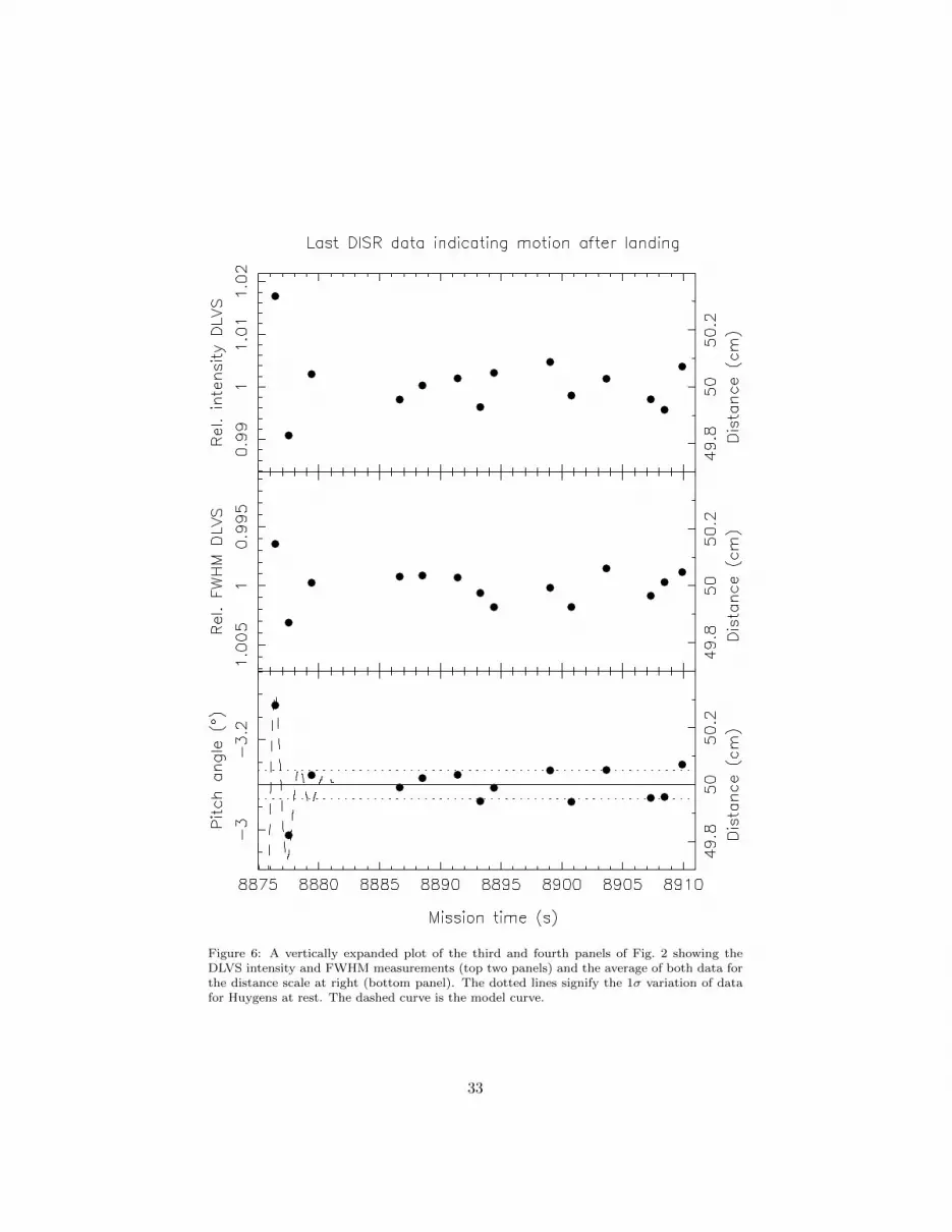
Figure 6: A vertically expanded plot of the third and fourth panels of Fig. 2 showing theDLVS intensity and FWHM measurements (top two panels) and the average of both data forthe distance scale at right (bottom panel). The dotted lines signify the 1σ variation of datafor Huygens at rest. The dashed curve is the model curve.

33

Figure 7: Top: HASI accelerometer data for the X- and Z-direction (solid curves representthe data smoothed with a 0.06 s FWHM Gaussian, raw data in gray) compared with ourmodel for Huygens’ motion (dashed curves). Bottom: The pitch angle variation as inferredby DISR instruments (symbols) and the model curve (dashed).

34

Figure 8: HASI acceleration data (top) and SSP tilt data (bottom) for both horizontal di-rections during the slide and wobble phase. The 1046 HASI data points are grouped as 23discrete data points. The data are quantized due to the relatively low resolution of the HASIpiezo-accelerometers. The number above each data point displays the frequency of occurrencefor that measurement. The dashed line connects averages for each of the eight verticallyaligned groups. The solid line is a linear fit, corresponding to a direction of motion 3◦ left ofthe Z-axis. The best linear fit for the tilt data has a slope of −33◦ degrees, which also corre-sponds to a motion vector 3◦ degrees left of the Z-axis considering that the SSP instrumentwas rotated by 30◦ degrees with respect to the principal axes of Huygens (Fig. 1).

35

Figure 9: Signal recorded by the SSP density sensor around the time of impact.

36

Figure 10: Huygens probe tilt around the time of impact as measured by the two SSP tiltsensors TIL X and TIL Y.

37

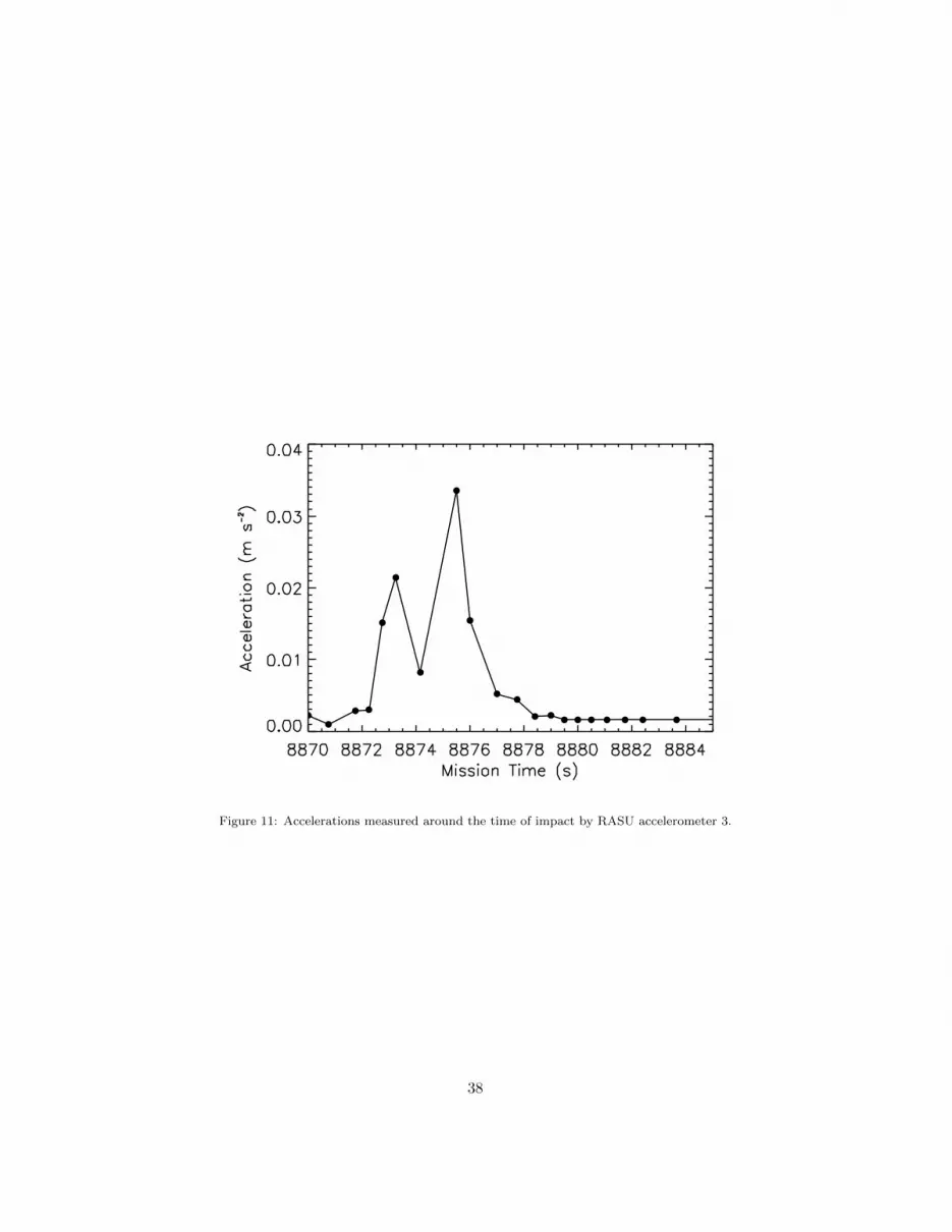
Figure 11: Accelerations measured around the time of impact by RASU accelerometer 3.

38

Figure 12: The Huygens SM2 model was dropped from a balloon as part of a test in Swedenin 1995. The plot shows the accelerations it experienced at impact; X is the vertical direction,Y and Z are lateral directions. The photo was taken after landing and shows impact markingsin the snow, annotated for clarity (photo: ESA).

39

Figure 13: The four phases around landing with three locations of the probe for each case andthe last phase for two alternative initial horizontal speeds. In each panel, the location of theprobe for three mission times is shown as indicated, in the temporal order of dotted, dashed,and solid outline. The bottom two panels show the inferred motion if the horizontal componentof the impact speed would have been v0Z = 0.67 or 0.66 m s−1 instead of 0.80 m s−1. Smalltick marks are spaced by 10 cm, large tick marks by 50 cm.

40

Figure 14: Horizontal speed data for the component in direction azimuth 115◦ (roughlyESE) around the time of landing from DWE data (left), DLIS data of the obstruction ofthe parachute (right), and from our model (bottom right). Note that the parachute datapoint applies for the motion of the parachute, not the probe. Error bars are indicated bydotted lines. The last 80 s before impact shown here correspond to the descent from 360 maltitude to the surface (calculated from an average descent speed of 4.5 m s−1).

41