Cryptanalysis of Discrete-Sequence SpreadSpectrum Watermarks
M. Kıvanc Mıhcak1, Ramarathnam Venkatesan1 and Mustafa Kesal2
1 Microsoft Research{kivancm,venkie}@microsoft.com
2 University of Illinois, [email protected]
Abstract. Assume that we are given a watermark (wm) embedding al-gorithm that performs well against generic benchmark-type attacks thatcomprise of simple operations that are independent of the algorithmand generally of the input as well. A natural question then is to askfor a nearly perfect cryptanalytic attack for the specific watermarkingmethod. In this paper we present and analyze an attack on a state-of-the-art Discrete-Sequence Spread Spectrum (dsss) audio watermarkingalgorithm. Our method uses detailed models for watermarked signal andalmost always jams or recovers > 90% of the watermarking-key. It ex-ploits the host and wm correlations, and the fact that one can locallycorrect errors in the wm estimates if the watermarking coefficients arediscrete. It is natural to use error-correction codes in a watermarkingalgorithm, and we study the effects of the accompanying redundancy aswell.
1 Introduction
Many wm embedding schemes use spread spectrum (ss) techniques [1], wheretypically the wm is an additive perturbation independent of the host signal. Weconsider a “blind private-key watermarking scheme”, where the detector knowsthe secret key, but not the the original host. The attacker knows everythingabout the watermarking algorithm, but has no access to the secret key, the hostdata or the detector itself.
We denote the host by s ∈ RN and the wm by m ∈ RN where mi ∈ B, whereB is a set of possible values. The wm m is usually generated pseudo-randomlyfrom some class of distributions using a random number generator, given a secretkey. Then, the watermarked signal is given by y ∈ RN, where y = s+m. At thedetector end, the goal is to successfully detect the existence of the wm in theinput signal. In dsss watermarking , B is a finite set. In this paper, we considerthe case B = {∆,−∆}. By key extraction, we mean computing m from y.
We call an attack against a given watermarking algorithm, an ε-perfectcryptanalytic attack (or ε-perfect attack for short) if with probability ≥ 1−ε,it (a) yields perceptually undistorted outputs and (b) removes wm . Barring suchan attack, a given watermarking algorithm may be useful in many circumstances.If a pirate has an attack that works, for example, only with 90% probability, he
will be exposed with ε = 10% probability, which limits his business model. Thus,ε-perfect attacks have a significantly higher threshold over generic benchmarkattacks. As we discuss next, it is non-trivial and can be hopeless to convert ageneric attack into a ε-perfect cryptanalytic attack.
Previous Work and Benchmarks The watermarking problem is often viewedas a communication problem with side information, where the message to betransmitted is the wm m and the side information is the host data s. If onewishes to account for adversaries, in particular with bounded computational re-sources (the only type of adversaries we are interested in), then this is no longera typical communication problem and is inextricably tied to computational com-plexity issues, which have little to do with the methods of communication andinformation theory. This issue has often been overlooked in the literature.
In addition, suggested (or tested) attacks are often independent of the partic-ular watermarking algorithm and do not fully exploit the available correlationsin the host and possibly in the wm in an adaptive manner, or information aboutthe particular targeted watermarking algorithm: usual attacks are non-malicioussuch as additive independent noise, denoising, smoothing, compression, rotation,cropping, shearing, etc [2, 3]. See [4] for a comprehensive survey.
With respect to most watermarking algorithms, some of which have charac-terizations of optimal attacks (which involves scaling and addition of Gaussianor other noise) and proofs that in their models that the attack can be withstood,Stirmark, with its fairly elementary methods, established an important point:they are vulnerable for reasons unclear or unaccounted for in the theoreticalmodel of their design. Using mathematically more sophisticated and remarkablysuccessful models and tools of signal processing (such as estimation, compres-sion, de-noising) for attacks is a natural variation and a motivation for morebenchmarks [3]. However, such benchmarks are at best sanity checks, and akin(in cryptography) to running randomness tests such as Diehard[5] or NIST’s[6](or applying favorite cryptanalytic tools [7] such as differential or linear analysis)to one’s latest cipher. There is no guarantee whatsoever such generic methodsapply to a targeted algorithm. For example, Checkmark as an attack on imagewatermarking algorithm [8] is comparable to jpeg compression; this image wa-termarking algorithm is yet to yield to targeted and specific estimation attacks,which are in part effective against plain dsss watermarking . It may be non-trivial to make it work near perfectly, for images, see website of [3] for someexamples.
We remark that issues here may be more complicated than in cryptogra-phy: both watermarking algorithms and attacks/benchmarks ail from the sameproblem: lack of a reasonably robust perceptual metric applicable in this con-text [9]. Furthermore, most of such attacks aim to jam the detector, rather thanextracting the key.
Contribution of our work : Assuming we are given a specific watermark-ing algorithm that is well engineered and performs remarkably well against awide-range of generic attacks, (e.g., audio analogies of those in [10]), a natural
and important question to decide the practical applicability of the algorithm isto ask if there is a ε-perfect attack. We studied a state of the art dsss audiowatermarking algorithm in [11] that embeds the wm which also uses error cor-recting codes for robustness. We study the algorithm for both hidden and knowncodebooks, with the goal of extracting the secret key, and as a byproduct get aε-perfect cryptanalytic attack with ε ∼ 0. Our attack exploits the host and wmcorrelations. We also implemented and tested an attack that does not recoversecret key, but was ε-perfect and used more detailed source models and in factmay be better for wider applicability since there may exist some watermarkingscheme for which it may be possible to jam, but not recover the key. Owing tospace constraints we do not describe this here.
We estimate the embedded wm and subtract a scaled version of the esti-mate from the watermarked data. This is similar to the so-called “remodulationattacks” in [10] and Wiener filtering in [12]; the non-trivial part is to derive amethod to perform this task for the targeted algorithm that is theoretically andempirically justifiable. In our results the attacked signal sounded closer to theoriginal than signal with the wm .
We use maximum a posteriori estimation which is optimal in the sense ofprobability of error (unlike the Wiener filter in [12] which is optimal only for sta-tionary Gaussian sources). Furthermore, we employ a Gaussian-based stochasticmodel for audio coefficients in the log-MCLT transform domain [13]. It is naturalto use error correcting codes in watermarking algorithms, and we analyticallycharacterize the tradeoff between the estimation accuracy and redundancy, andprovide experimental results on the success of the proposed attack. Moreover, weprecisely quantify the performance of the attack in a detection-theoretic sense.We are not aware of such a discussion in related literature (see [10, 12] or theirreferences).
Outline of the paper: In section 2 we give an overview of the method. Sec-tion 3 explains our source model, section 4 analyzes correlation detectors fordsss watermarking schemes, section 5 describes the key extraction and section6 presents the attack and quantifies the degradation of the detector. Section 7describes the method’s empirical effectiveness against [11]: our key extractionalmost always recovers > 90% of the key. For further details, see [14]; we omitour experimental results on images for ss watermarking schemes with no repeti-tion and our attacks are not yet effective against watermarking methods whichuse explicit randomization and choose watermarking pseudo-randomly from aninterval[8].
Notation : We are going to use calligraphic letters for sets, | . | operatorfor the cardinality of sets, superscripts to index set elements, boldface lettersfor vectors, and corresponding regular letters with subscripts to index elementsof vectors. For example, consider set A where A =
{a1,a2, . . . ,a|A|
}and aj
i
denotes the i-th element of vector aj . Also let N (µ, σ2
)denote the Gaussian
distribution with mean µ and variance σ2, log stand for the natural logarithmand < . , . > represent the inner product corresponding to Euclidean norm.Further notation shall be introduced in Secs. 2, 3 and 4, wherever applicable.
2 Overview of the Proposed Attack
Our attack consists of two steps:
1. Given y, we produce an estimate m of the wm m using models that exploitcorrelations in the watermarked image and the wm if any;
2. An estimate for input signal is now made; for example, one can use z =y − αm where α > 0 is an input parameter and y is the input to the wmdetector.
For step 1, one can use various methods to suit different source models. Agood estimate for wm depends on the specific watermarking algorithm itself,in particular the structure of the codeword set M⊆ {∆,−∆}N from which thewm m is chosen. Obviously, more accurate estimation will make the attack moreeffective. On the other hand, the estimation accuracy in step 1, depends on theamount of redundancy used in the design of the codeword set M. The redun-dancy can be used in the form of repetitions as in most ss based watermarkingalgorithms. We remark that it is safe for the designers to assume that (i.e., unsafeto assume the contrary) if repetitions help the watermarking detector quanti-tatively (in terms of robustness against common signal processing attacks), itis likely to help the attack as well. As for a good defense, we suggest explicitrandomization of the steps in watermarking algorithm (e.g. as in [8, 15]).
3 Source Model
We assume that the host data is a realization of conditionally independent Gaus-sian distribution (conditioned on the parameters of the Gaussian distribution).The parameters of the Gaussian distribution can be heavily correlated. Notethat, in terms of the assumptions about the source distribution, there is a signif-icant difference between the watermarking algorithm designer and the attacker.The designers could possibly design the wm encoding algorithm based on asource distribution, however from a security perspective it is inherently danger-ous to design a watermarking detector relying on a source distribution, since anattacker can in principle “skew” or “bend” the distribution so as to force thedetector to produce unwanted outputs. On the other hand, the situation is moreor less the opposite for attackers. This is because a fixed watermarking algorithmcannot easily ensure that the outputs do not obey a class of distributions. Hencethe attack analysis presented here has its importance as it clarifies the algorithmand points some subtleties.
Let the unwatermarked source data be s, a length-N zero mean Gaussianvector whose elements are conditionally independent (conditioned on the vari-ances). Throughout the text, we drop the conditioning from notation for thesake of simplicity. The correlations in the source are embedded in the correla-tions between the variances. As a result, we propose a locally i.i.d. (independentidentically distributed) source model. Under this model we assume that s consistsof segments of length M where N = qM , both q and M are positive integers.
Within segment i, s is assumed to be i.i.d. Gaussian with variance σ2i , 1 ≤ i ≤ q,
i.e., sj ∼ N (0, σ2
i
), (i − 1)M + 1 ≤ j ≤ iM , 1 ≤ i ≤ q, where j ∈ {1, . . . N}.
Then, we have
p (s) =q∏
i=1
iM∏
j=(i−1)M+1
1√2πσi
exp
(− s2
j
2σ2i
),
and
log p (s) = −12
q∑
i=1
M log(2πσ2
i
)− 12
q∑
i=1
iM∑
j=(i−1)M+1
s2j
σ2i
,
where p(.) is the corresponding probability density function. Variants of thismodel have been shown to be quite useful within the context of image compres-sion [16] and image denoising [17].
4 On dsss Watermarking Methods
Let m ∈ M be the wm vector (message) which is chosen randomly (underuniform distribution) from the “codeword set” M where M⊆ {∆,−∆}N (ran-domization is carried out using the secret key as the seed of the random numbergenerator). For dsss methods, watermarking rule is defined by y = s+m whereaddition is component-wise and y is the watermarked signal.
At the detector end, the purpose is to reliably detect the presence of wm .Under private key blind watermarking scenario, it is assumed that the detectorknows the secret key and M, hence m, however it does not know s. Under theseconditions, the detector provides a solution to the following binary hypothesistesting problem :
H0 : y = s
H1 : y = s + m
In this paper, we consider the detectors that use “correlation test”, since thisis usually the detection rule that is used in the literature for sswatermarkingschemes3. The correlation detector is given by
N∑
i=1
yimi
H1
><H0
τ (4.1)
Next, we derive the performance of the correlation detector using our sourcemodel.3 It can be shown that the correlation detector is not optimal (in the sense of probabil-
ity of error) in general for non-i.i.d. host signals. The optimality holds only for i.i.d.Gaussian host signals. The performance loss due to suboptimality of the correlationdetector shall be quantified in our future work
Within a detection-theoretic setting, the performance of the detector is char-acterized by PF (probability of false alarm) and PM (probability of miss)[18],where
PF4= Pr [deciding on H1|H0]
andPM
4= Pr [deciding on H0|H1] .
Using rule (4.1), PF = Pr[∑N
i=1 yimi > τ |H0
]and PM = Pr
[∑Ni=1 yimi < τ |H1
].
Under H0, we have∑N
i=1 yimi ∼ N (0,∆2M
∑qi=1 σ2
i
)and hence
PF = Q
(τ
∆√
M√∑q
i=1 σ2i
), (4.2)
where Q(t)4=
∫∞t
1√2π
exp(−u2/2
)du. Under H1, we have
∑Ni=1 yimi ∼ N (
N∆2,∆2M∑q
i=1 σ2i
)and hence
PM = Q
(N∆2 − τ
∆√
M√∑q
i=1 σ2i
). (4.3)
The results (4.2) and (4.3) shall be useful in the subsequent sections in order toevaluate the degradation in the performance of the detector after the proposedattack. In the next section, we outline our attack approach and provide a briefdiscussion. In Secs. 5 and 6, we explain the details of our approach and derivethe related results.
5 Key Extraction
We use ML estimation to extract the key. We assume that the estimation ofwm will be carried out on watermarked data only, i.e., we assume that theattacker is aware of the presence of a wm and hence, the attack is applied onlyto watermarked signals. Moreover, we assume that the attacker knows everythingabout the wm embedding algorithm, except for the secret key, i.e., the attackerknows the domain where wm is embedded, the magnitude of wm samples, ∆ andthe setM from which wm is selected; however he does not know the wm sequenceitself. Furthermore, we assume that the total wm m consists of concatenation ofwm vectors
{w(i)
}where w(i) is the wm for segment i, and w(i) is chosen from
set W ⊆ {∆,−∆}M , 1 ≤ i ≤ q.First note that, according to MAP (Maximum A Posteriori) rule, the esti-
mation problem ismMAP = argmax
m∈Mp (y|m) f (m) ,
where f(.) is the probability density function according to which codewords areselected from M. Now, we assume that the choice of a particular wm from set
M bears no bias over another one. In that case f (m) = 1/ |M|, ∀m ∈ M andthe MAP rule reduces to ML rule :
mML = argmaxm∈M
p (y|m) . (5.4)
Next, we show that under the assumptions stated above, it is optimal to carryout estimation locally within each segment independent of other segments.
Lemma 1. The choice of[w(1)
MLw(2)ML . . . w(q)
ML
]is a solution to (5.4) where for
each i w(i)ML is a solution to
w(i)ML = argmax
w∈Wp
(y(i)|w
)= argmax
w∈Wlog p
(y(i)|w
). (5.5)
where y(i) is the watermarked data in segment i, 1 ≤ i ≤ q.
Proof : See Appendix A.
5.1 Estimation Analysis - Most General Case
In this section, our goal is to quantify the accuracy of the estimator in termsof finding the probability distribution of the number of wm samples that areestimated inaccurately. Due to Lemma 1, it is optimal to carry out estimationindependently in each segment. Thus, we shall follow this procedure. In thissection, we will confine our analysis to a single segment. However the resultspresented here can be extended to the total signal without difficulty once thestructure of W is known. For convenience, we drop the superscripts of type (i)that index the segments in this section. Let σ2 be the variance of each sj withinsegment i. In the most general case, our goal is to solve the following discreteoptimization problem for each segment
wML = argmaxw∈W
log p (y|w) , (5.6)
where W ={w1,w2, . . . ,w|W|}. Since p (yi|wi) ∼ N (
wi, σ2),
wML = argmaxw∈W
[−M
2log
(2πσ2
)− 12σ2
M∑
i=1
(yi − wi)2
](5.7)
= argmaxw∈W
< y,w >, (5.8)
where the last equality follows since w2i = ∆2 is constant, 1 ≤ i ≤ M .
Before stating the result, first we introduce the following definitions:
– e4= number of bits that are estimated incorrectly within a segment.
– pij4= Pr
[wML = wi|w = wj
](conditional probability of getting wi as a re-
sult of ML estimation where wj was actually embedded).
– dij4= 1
2∆
∑Mk=1
∣∣∣wik − wj
k
∣∣∣ (normalized l1 distance between wi and wj , also
can be viewed as the Hamming distance between “variants” of wi and wj
in GF2). Note that 1 ≤ dij ≤ M for i 6= j.– Aj
k ={wi ∈ W|dij = k
}, 0 ≤ k ≤ M (the set of codewords which are at
distance k from wj). Note that Aj0 =
{wj
}, 1 ≤ j ≤ |W|, ⋃M
k=0Ajk = W, ∀j.
– M × 1 vector ai where aik
4= < s,wi −wk >, 1 ≤ k ≤ M .
– M × 1 vector bij where bijk
4= < wi,wj > − < wk,wj >, 1 ≤ k ≤ M .
– Ri 4= E[aiaiT
](autocorrelation matrix of ai).
Now, we present Lemma 2 where we quantify the results of wm estimation inthe most general case and provide closed form expressions for estimation error.Lemma 2 presents closed form expressions for:
– Conditional probability of estimating wj where wi is actually embedded (i.e.pij).
– The probability distribution of the error made as a result of the estimation(i.e., the probability distribution of e)
Lemma2.(i) pij = Pr
[ai
k + bijk ≥ 0, 1 ≤ k ≤ M
]where ai
k ∼ N (0, 4∆2σ2dik
)and bij
k =
2∆2 (dkj − dij).(ii) Assuming that Ri is strictly positive definite, there exists an eigenvector
decomposition Ri = ViΛiViT such that pij =∏M
k=1 Q(− bij
k√λi
k
)where bij =
ViT bij and λik is the k-th element of Λi along the diagonal.
(iii) Pr[e = k|w = wj
]=
∑i s.t.wi∈Aj
kpij and
Pr [e = k] = 1|W|
∑|W|j=1
∑i s.t.wi∈Aj
kpij.
Proof : See Appendix B.
Naturally the characteristic of the estimation error depends on the structureof the codeword set W. In general it is a nontrivial task to find the these char-acteristics (pij and Pr [e = k]) for arbitrary codeword sets W. In this paper, weconcentrate on the special case of “block repetition codes”, i.e., the case when∆ or −∆ is repeated within each segment. As a result, we derive tractable ex-pressions for the distribution of the error that is made in the estimation process.More detailed analysis on different codes shall be considered in our future work.
5.2 Estimation Analysis - Block Repetition Code
In this section, we consider the case where W ={w0,w1
}where w0
k = −∆,w1
k = ∆, 1 ≤ k ≤ M .
Lemma 3.If W =
{w0,w1
}, for segment k, p01 = p10 = Q
(∆σk
√M
), p00 = p11 = 1− p01,
Pr [e = 0] = p00, Pr [e = M ] = p01, where σ2k is the variance of segment k,
1 ≤ k ≤ q.
Proof : See Appendix C.
Now, we extend the estimation error result to the whole signal under ourlocally i.i.d. source model for the block repetition code case. Let
Bk 4= {(l1, l2, . . . , lk) |li 6= lj fori 6= j and li ∈ {1, 2, . . . , q} , 1 ≤ i ≤ k} ,
1 ≤ k ≤ q with B0 4= ∅ (i.e., Bk is the set of all possible k–tuples from the set
{1, 2, . . . q}. Note that∣∣Bk
∣∣ =(
qk
). Also let etotal be the number of bits that
are estimated incorrectly in the whole signal. Then we have the following result.
Corollary 4.
Pr [etotal = kM ] =∑
(l1,...,lk)∈Bk
[k∏
m=1
Q(
∆
σlm
√M
) q∏
m=k+1
[1−Q
(∆
σlm
√M
)]].
Corollary 4 is immediate from the independence of codeword selection betweendifferent segments.Remark : Clearly, the wm estimation process will perform strictly better than50% (i.e., in expectation sense strictly more than half of the watermarkingbits shall be estimated correctly). The estimation accuracy depends on rela-tive strength of the wm with respect to the signal as well as the wm length andthe particular codebook used. For instance, the usage of block repetition codesgreatly increases the estimation accuracy. Also as the wm strength increases, theestimation error would in general decrease. Note that, some controlled redun-dancy and relatively strong wms are usually essential in ss based watermarkingschemes in order to provide synchronization against de–synch attacks and with-stand against common signal processing attacks. This redundancy is usuallyprovided in terms of using a block repetition code in the watermarking commu-nity. Such a watermarking scheme, if designed properly, is expected to withstandmost reasonable “blind” attacks (such as de–synchronization attacks, band passfiltering, compression, denoising, etc.), that aim to jam the detector only. Weuse the term “blind” for an attack if the attack does not make use of the wa-termarking algorithm used in the system. In general, as a rule of thumb, as theamount of redundancy in the watermarking code and the strength of the wmincrease, the robustness against blind attacks is expected to increase. On theother hand, this also brings advantages to a “non–blind” attacker (a non–blindattacker is an attacker that knows the watermarking algorithm completely orhas some partial information about the watermarking algorithm), who aims toextract the key.
6 Analysis of the Proposed Attack
Our proposed attack produces the following signal:
z = y − αmML = s + m− αmML. (6.9)
Since the attacker is going perform strictly better than “random coin flips”in expectation sense, clearly if α is chosen large enough, the wm detector isexpected to fail. If the estimation accuracy is high (say around %90) α ∼ 1 wouldbe sufficient. However, as the estimation accuracy degrades (i.e., gets closer to%50), it would be necessary to use higher values of α in order to increase thePM of detector to a desired level. On the other hand, if α is too large, theattacker is going to introduce unacceptable amount of distortion to the signal.In this section, our goal is to quantify this trade–off. In particular, in Sec. 6.1, wequantify the distortion introduced by the proposed attack in an expected MSE(mean squared error) sense. In Sec. 6.2, we quantify the degradation in wmdetection by analyzing the variations in PF and PM of a correlation detectorof a dsss scheme after proposed attack. We provide results for block repetitioncodes.
6.1 Distortion Induced by Proposed Attack
Letdtotal
4= z− s = m− αmML
be the total distortion vector introduced by the attack. Our goal in this sectionis to find E ||dtotal||2. First, we derive the expected MSE in a particular seg-ment. This result can easily be generalized to the whole signal. Afterwards, wespecialize to the case of block repetition codes.
Lemma5. Within a particular segment,
E ||d||2 = ∆2M(1 + α2
)+ 2α∆2
−M +
2|W|
|W|∑
i=1
|W|∑
j=1
dijpij
, (6.10)
where d = w − αwML and pij = Pr[wML = wi|w = wj
]within that segment
and dij is the “Hamming distance” between wi and wj (as defined in Sec. 5.1).
Proof : See Appendix D.
Corollary 6. In the block repetition code case, i.e., W ={w0,w1
}, where w0
l =−∆, w1
l = ∆, 1 ≤ l ≤ M , we have
E ||d||2 = ∆2M
[1 + α2 + 2α
(2Q
(∆
σk
√M
)− 1
)], (6.11)
in segment k, and
E ||dtotal||2 = ∆2N[1 + α2
]+ ∆2M2α
(−q + 2
q∑
k=1
Q(
∆
σk
√M
)). (6.12)
Proof : See Appendix E.
6.2 Degradation of wm Detection after Proposed Attack
Now, we quantify the degradation in the performance of the wm detector, whichuses correlation test. First recall that we assume the attacker is aware of thepresence of the wm i.e., proposed estimation attack is applied only if the inputsignal is watermarked. Therefore, PF (i.e., probability of detecting wm if wmis not embedded) does not change after the attack. The proposed attack onlychanges PM (i.e., probability of declaring wm is not present even though wm wasembedded). In order to gain insight, we first consider the simplest case, wherewe consider a single Gaussian random variable. We are able to find tractableclosed form expressions in this case. Then, we extend this result to the case ofblock repetition codes and provide tractable lower bounds on PM .
Single Random Variable Case Consider a single Gaussian random variables, that is watermarked via dsss : y = s + w, w is randomly chosen from W ={∆,−∆} with a fair coin toss. The detector applies the simple correlation test;then the decision rule is
yw
H1
><H0
τ,
where PM = Pr [yw < τ |y = s + w] = Q(
∆2−τ∆σ
)and σ2 is the variance of s. The
estimation attack produces w = ∆signy. After the attack, the detector input isz = y − αw = s + w − αw. Let E 4= zw = sw + ∆2 − αww.
Lemma 7. For the single random variable setup,
PM = Pr [E < τ ] =
Q(
∆2(1+α)−τ∆σ
)−Q
(∆σ
)+ Q
(∆2(1−α)−τ
∆σ
)if ∆2α > τ
Q(
∆2(1−α)−τ∆σ
)else
.
(6.13)
Proof : See Appendix F.Remark : There is a nonuniform behavior in the functional behavior of PM .There are 2 regions (2 different functional forms); these regions are determinedby comparing ∆2α with τ . It can be shown that PM is an increasing function ofα, however the rate of increase changes in the regions of ∆2α > τ and ∆2α ≤ τ .In particular it can be shown that when ∆2α ≤ τ , PM increases a lot faster withrespect to α than the other regime. Hence, for fixed τ , an increase in ∆2α is veryuseful for attacker (since the rate of increase in PM increases), i.e. increasing wmstrength (∆) and/or attack strength (α) benefits the attacker. Also, for fixed ∆
and α, decreasing τ damages the attackers performance. However, note that, asτ decreases, the chances of declaring unwatermarked data as watermarked (i.e.,PF ) increases, which is not shown here.
Block Repetition Code Case Now, consider the case where block repeti-tion code is used within each segment. Due to our locally i.i.d. model, thiscase can be viewed as watermarking the length–q signal (recall that q is thenumber of segments) s, which is given by the local averages of s. Hence, si =1M
∑iMj=(i−1)M+1 sj , and si ∼ N (
0, σ2i /M
)for segment i, where 1 ≤ i ≤ q. Fur-
thermore let y be the length q signal that consists of arithmetic means of thewatermarked signal y for each segment, i.e., yi = 1
M
∑iMj=(i−1)M+1 yj , 1 ≤ i ≤ q.
Then for segment i, if w = w0 (w = w1), then clearly yi = si−∆ (yi = si +∆).Hence, the whole setup can be viewed as attacking the watermarked signal y,where no ECC (error correction coding) has been used in the wm generation.Utilizing this approach, we can use the result of Lemma 7 in deriving probabilityof error results for the block repetition code case. Thus, we present the followingresult.
Corollary 8. When W ={w0,w1
}, where w0
k = −∆, w1k = ∆, 1 ≤ k ≤ M ,
according to 0–mean locally i.i.d. Gaussian model with variance σ2i in segment
i, 1 ≤ i ≤ q, N = qM , we have the following:(i) For segment i, we have
PM =
Q(√
M ∆2(1+α)−τ∆σi
)−Q
(√M ∆
σi
)+ Q
(√M ∆2(1−α)−τ
∆σi
)if ∆2α > τ
Q(√
M ∆2(1−α)−τ∆σi
)else
.
(6.14)(ii) Let Dk be the set of all k–tuples from index set {1, 2, . . . , q}, i.e.,
Dk 4={vkl|vkl
i 6= vklj for i 6= j and vkl
i ∈ {1, . . . , q} , 1 ≤ i ≤ k, 1 ≤ l ≤ |Dk| =(
qk
)}.
Accordingly define the index set of vkl (i.e., elements of the l-th k-tuple from setDk):
Vkl 4={vkl0 , vkl
1 , . . . , vklk
}.
Also let Vkl,C denote {1, . . . , q} − Vkl. Then for the whole signal we have
PM =N∑
k=0
|Dk|∑
l=1
Pr
[q∑
i=1
si >q∆2 (1 + α)− τ − 2kα∆2
∆, sm < ∆, m ∈ Vkl,
sn > ∆, n ∈ Vkl,C]
(6.15)
≥q∑
k=d 12 (q− τ
α∆2 )e
{(qk
)[Q
(√M
q∆2 (1 + α)− τ − 2kα∆2
q∆σmin
)−Q
(√M
∆
σmin
)]k
[Q
(√M
∆
σmin
)]q−k}
, (6.16)
where σmin4= min1≤i≤q σi.
The results (6.14) and (6.15) follow directly from the extension of (6.13).In order to obtain (6.16), we use union bound and monotonicity properties ofthe Q (·) function. The complete proof has been omitted here due to space con-straints.
7 Practical Applications
We developed 3 variants of our attack approach and applied them on the state-of-the-art audio watermarking algorithm [11], which was designed using dssssignal watermarking approach.
7.1 An Overview of the Tested Audio watermarking Scheme [11]
Here, we provide an outline of [11]. Some of the pre– and post–processing detailsare omitted due to space constraints. Both wm embedding and detection takesplace in the time–frequency representation of the audio clip. In particular MCLT(Modulated Complex Lapped Transform) has been used in order to pass to thisdomain [13]. 8 bits are hidden in a L = 11 second audio clip. The first 4 bitsare used for randomization purposes together with the secret key. The last 4bits are actually embedded after the randomization process. An L second audioclip is divided into “cells” in the time–frequency domain. There are total of 120splits along the frequency axis and 24 splits along the time axis. The splittingalong the time axis is done in a uniform fashion whereas the splitting along thefrequency axis is done in a geometric progression. In the embedding process acodeword set C is used. The set C has the following properties:
– C ∈ {∆,−∆}6– |C| = 12– c ∈ C ⇔ c ∈ C where c is defined such that ci = −ci, 1 ≤ i ≤ 6.
Now for each frequency split (there are 120 of them), there are 24 cells to con-sider. These cells are divided into 4 groups (because there are 4 bits to embed),6 cells in each group. 1 bit falls to each group. Given 1 bit, an element c is cho-sen randomly from C. Then, the chosen c is embedded to each group by usingthe block repetition code, i.e., ci ∈ {∆,−∆} is embedded in the i–the cell ofthe group. The addition of ±∆ is done in the magnitude MCLT domain afterapplying log non–linearity. The detector uses the correlation test. The frequencyband, that is used both in wm embedding and detection, is 2–7 kHz band. Forfurther details, we refer the reader to [11].
7.2 Simulation Results Based on Quantitative Analysis of theAttack
Now, we present predictions about proposed attack for the setup of [11] bynumerically evaluating our theoretic results that were derived in the previous
sections. Our experiments revealed that, the variance of MCLT coefficients (usingon a 0-mean locally i.i.d. Gaussian model) were in the range of 4−6 most of thetime (after applying the proper pre-processing mentioned in [11]). Also averagecell size for proposed method was about 40 coefficients. In [11], ∆ is typicallychosen in the range of [1, 3]. ∆ = 1 is used for numerical simulations of ouranalysis.
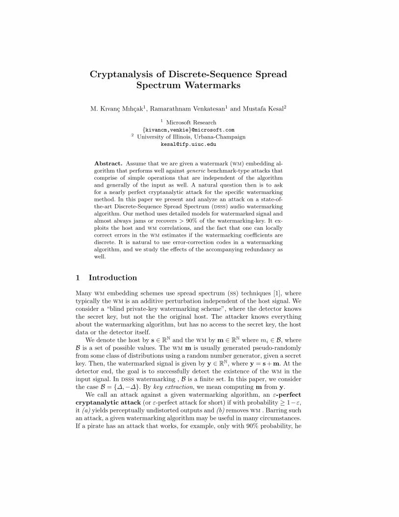
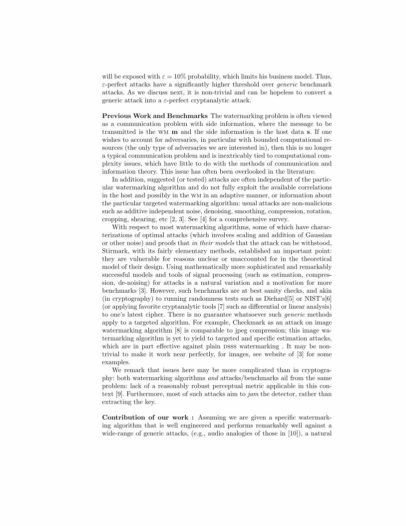
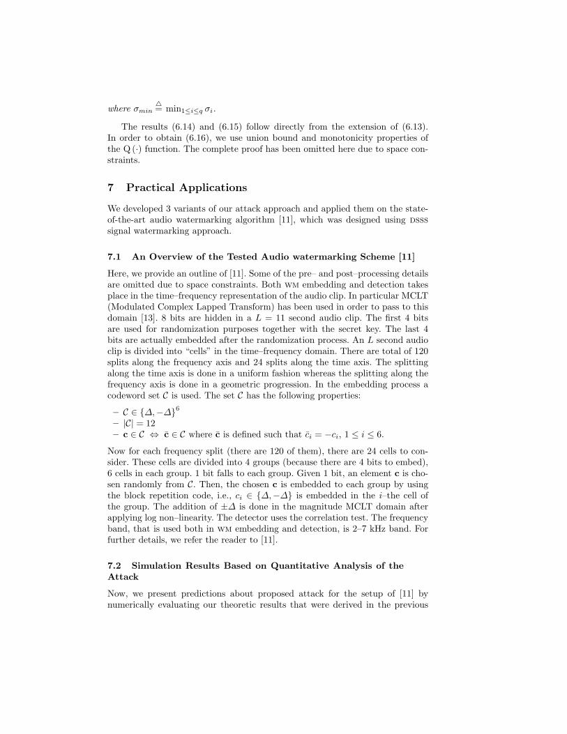
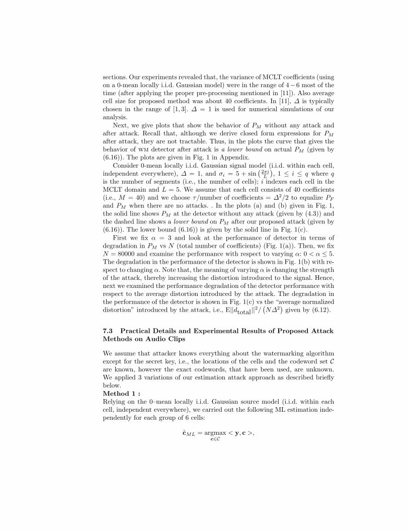
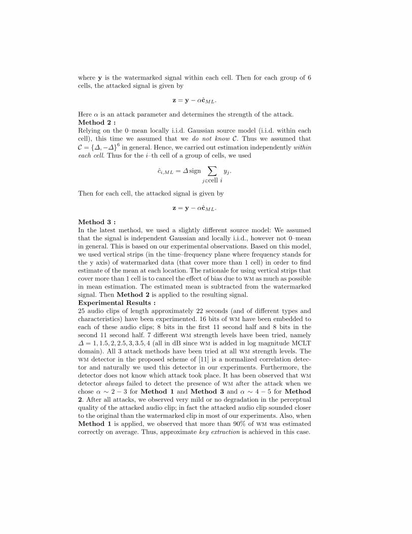
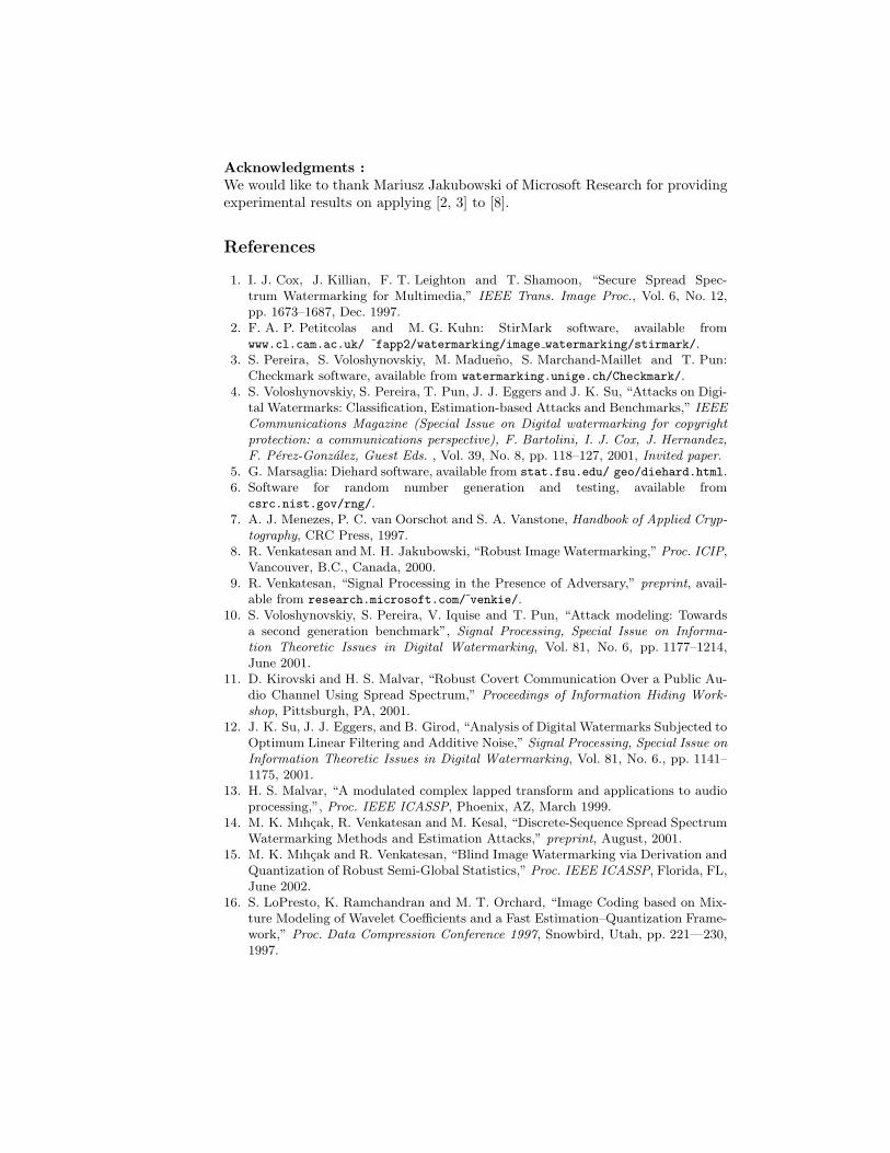
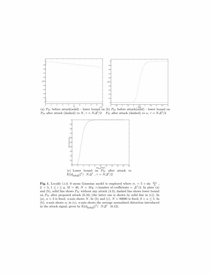
Next, we give plots that show the behavior of PM without any attack andafter attack. Recall that, although we derive closed form expressions for PM
after attack, they are not tractable. Thus, in the plots the curve that gives thebehavior of wm detector after attack is a lower bound on actual PM (given by(6.16)). The plots are given in Fig. 1 in Appendix.
Consider 0-mean locally i.i.d. Gaussian signal model (i.i.d. within each cell,independent everywhere), ∆ = 1, and σi = 5 + sin
(2πiL
), 1 ≤ i ≤ q where q
is the number of segments (i.e., the number of cells); i indexes each cell in theMCLT domain and L = 5. We assume that each cell consists of 40 coefficients(i.e., M = 40) and we choose τ/number of coefficients = ∆2/2 to equalize PF
and PM when there are no attacks. . In the plots (a) and (b) given in Fig. 1,the solid line shows PM at the detector without any attack (given by (4.3)) andthe dashed line shows a lower bound on PM after our proposed attack (given by(6.16)). The lower bound (6.16)) is given by the solid line in Fig. 1(c).
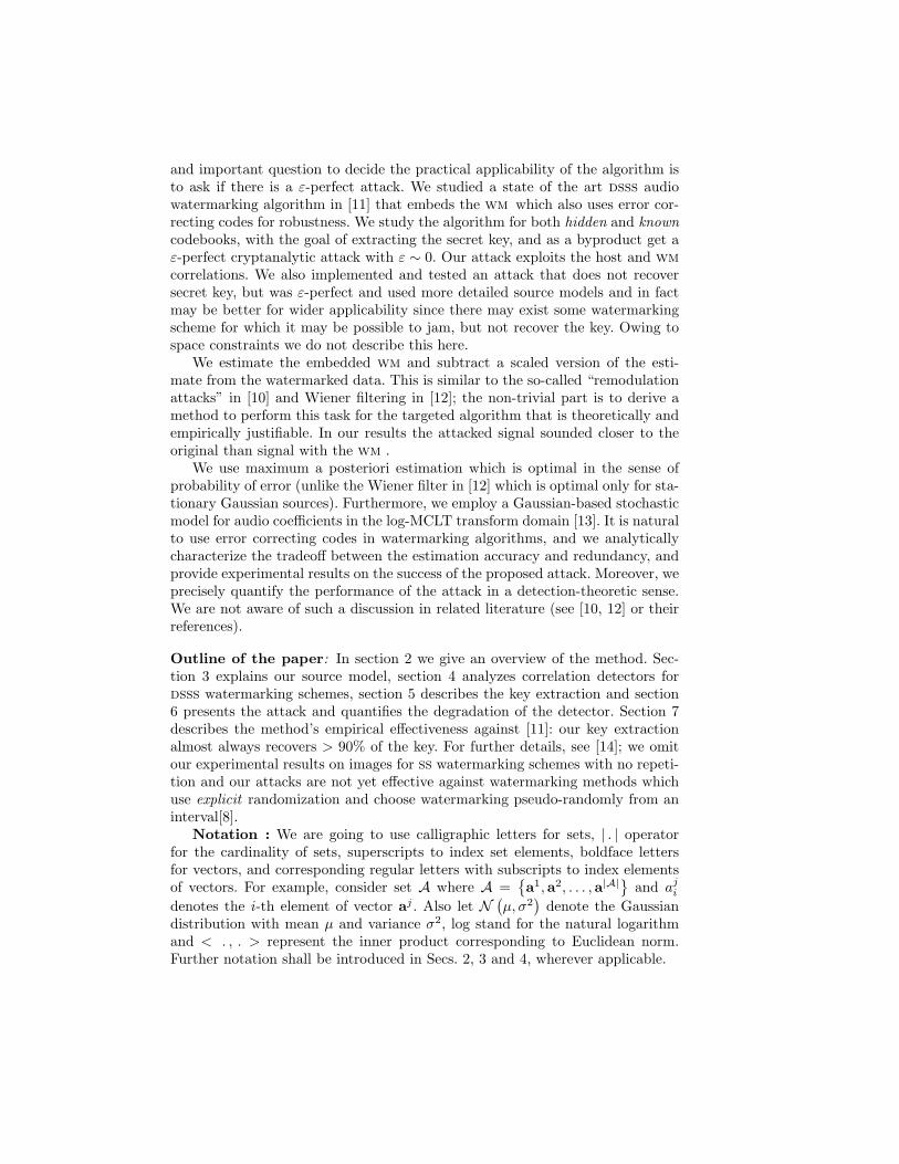
First we fix α = 3 and look at the performance of detector in terms ofdegradation in PM vs N (total number of coefficients) (Fig. 1(a)). Then, we fixN = 80000 and examine the performance with respect to varying α: 0 < α ≤ 5.The degradation in the performance of the detector is shown in Fig. 1(b) with re-spect to changing α. Note that, the meaning of varying α is changing the strengthof the attack, thereby increasing the distortion introduced to the signal. Hence,next we examined the performance degradation of the detector performance withrespect to the average distortion introduced by the attack. The degradation inthe performance of the detector is shown in Fig. 1(c) vs the “average normalizeddistortion” introduced by the attack, i.e., E||dtotal||2/
(N∆2
)given by (6.12).
7.3 Practical Details and Experimental Results of Proposed AttackMethods on Audio Clips
We assume that attacker knows everything about the watermarking algorithmexcept for the secret key, i.e., the locations of the cells and the codeword set Care known, however the exact codewords, that have been used, are unknown.We applied 3 variations of our estimation attack approach as described brieflybelow.Method 1 :Relying on the 0–mean locally i.i.d. Gaussian source model (i.i.d. within eachcell, independent everywhere), we carried out the following ML estimation inde-pendently for each group of 6 cells:
cML = argmaxc∈C
< y, c >,
where y is the watermarked signal within each cell. Then for each group of 6cells, the attacked signal is given by
z = y − αcML.
Here α is an attack parameter and determines the strength of the attack.Method 2 :Relying on the 0–mean locally i.i.d. Gaussian source model (i.i.d. within eachcell), this time we assumed that we do not know C. Thus we assumed thatC = {∆,−∆}6 in general. Hence, we carried out estimation independently withineach cell. Thus for the i–th cell of a group of cells, we used
ci,ML = ∆ sign∑
j∈cell i
yj .
Then for each cell, the attacked signal is given by
z = y − αcML.
Method 3 :In the latest method, we used a slightly different source model: We assumedthat the signal is independent Gaussian and locally i.i.d., however not 0–meanin general. This is based on our experimental observations. Based on this model,we used vertical strips (in the time–frequency plane where frequency stands forthe y axis) of watermarked data (that cover more than 1 cell) in order to findestimate of the mean at each location. The rationale for using vertical strips thatcover more than 1 cell is to cancel the effect of bias due to wm as much as possiblein mean estimation. The estimated mean is subtracted from the watermarkedsignal. Then Method 2 is applied to the resulting signal.Experimental Results :25 audio clips of length approximately 22 seconds (and of different types andcharacteristics) have been experimented. 16 bits of wm have been embedded toeach of these audio clips; 8 bits in the first 11 second half and 8 bits in thesecond 11 second half. 7 different wm strength levels have been tried, namely∆ = 1, 1.5, 2, 2.5, 3, 3.5, 4 (all in dB since wm is added in log magnitude MCLTdomain). All 3 attack methods have been tried at all wm strength levels. Thewm detector in the proposed scheme of [11] is a normalized correlation detec-tor and naturally we used this detector in our experiments. Furthermore, thedetector does not know which attack took place. It has been observed that wmdetector always failed to detect the presence of wm after the attack when wechose α ∼ 2 − 3 for Method 1 and Method 3 and α ∼ 4 − 5 for Method2. After all attacks, we observed very mild or no degradation in the perceptualquality of the attacked audio clip; in fact the attacked audio clip sounded closerto the original than the watermarked clip in most of our experiments. Also, whenMethod 1 is applied, we observed that more than 90% of wm was estimatedcorrectly on average. Thus, approximate key extraction is achieved in this case.
Acknowledgments :We would like to thank Mariusz Jakubowski of Microsoft Research for providingexperimental results on applying [2, 3] to [8].
References
1. I. J. Cox, J. Killian, F. T. Leighton and T. Shamoon, “Secure Spread Spec-trum Watermarking for Multimedia,” IEEE Trans. Image Proc., Vol. 6, No. 12,pp. 1673–1687, Dec. 1997.
2. F. A. P. Petitcolas and M. G. Kuhn: StirMark software, available fromwww.cl.cam.ac.uk/ fapp2/watermarking/image watermarking/stirmark/.
3. S. Pereira, S. Voloshynovskiy, M. Madueno, S. Marchand-Maillet and T. Pun:Checkmark software, available from watermarking.unige.ch/Checkmark/.
4. S. Voloshynovskiy, S. Pereira, T. Pun, J. J. Eggers and J. K. Su, “Attacks on Digi-tal Watermarks: Classification, Estimation-based Attacks and Benchmarks,” IEEECommunications Magazine (Special Issue on Digital watermarking for copyrightprotection: a communications perspective), F. Bartolini, I. J. Cox, J. Hernandez,F. Perez-Gonzalez, Guest Eds. , Vol. 39, No. 8, pp. 118–127, 2001, Invited paper.
5. G. Marsaglia: Diehard software, available from stat.fsu.edu/ geo/diehard.html.6. Software for random number generation and testing, available from
csrc.nist.gov/rng/.7. A. J. Menezes, P. C. van Oorschot and S. A. Vanstone, Handbook of Applied Cryp-
tography, CRC Press, 1997.8. R. Venkatesan and M. H. Jakubowski, “Robust Image Watermarking,” Proc. ICIP,
Vancouver, B.C., Canada, 2000.9. R. Venkatesan, “Signal Processing in the Presence of Adversary,” preprint, avail-
able from research.microsoft.com/ venkie/.10. S. Voloshynovskiy, S. Pereira, V. Iquise and T. Pun, “Attack modeling: Towards
a second generation benchmark”, Signal Processing, Special Issue on Informa-tion Theoretic Issues in Digital Watermarking, Vol. 81, No. 6, pp. 1177–1214,June 2001.
11. D. Kirovski and H. S. Malvar, “Robust Covert Communication Over a Public Au-dio Channel Using Spread Spectrum,” Proceedings of Information Hiding Work-shop, Pittsburgh, PA, 2001.
12. J. K. Su, J. J. Eggers, and B. Girod, “Analysis of Digital Watermarks Subjected toOptimum Linear Filtering and Additive Noise,” Signal Processing, Special Issue onInformation Theoretic Issues in Digital Watermarking, Vol. 81, No. 6., pp. 1141–1175, 2001.
13. H. S. Malvar, “A modulated complex lapped transform and applications to audioprocessing,”, Proc. IEEE ICASSP, Phoenix, AZ, March 1999.
14. M. K. Mıhcak, R. Venkatesan and M. Kesal, “Discrete-Sequence Spread SpectrumWatermarking Methods and Estimation Attacks,” preprint, August, 2001.
15. M. K. Mıhcak and R. Venkatesan, “Blind Image Watermarking via Derivation andQuantization of Robust Semi-Global Statistics,” Proc. IEEE ICASSP, Florida, FL,June 2002.
16. S. LoPresto, K. Ramchandran and M. T. Orchard, “Image Coding based on Mix-ture Modeling of Wavelet Coefficients and a Fast Estimation–Quantization Frame-work,” Proc. Data Compression Conference 1997, Snowbird, Utah, pp. 221—230,1997.
17. M. K. Mıhcak, I. Kozintsev, K. Ramchandran and P. Moulin, “Low-ComplexityImage Denoising Based on Statistical Modeling of Wavelet Coefficients,” IEEESignal Processing Letters, Vol. 6, No. 12, pp. 300—303, Dec. 1999.
18. H. L. Van Trees, Detection, Estimation and Modulation Theory, Wiley, 1968.
APPENDIX
A Proof of Lemma 1
The optimization problem (5.4) can be rewritten as mML = argmaxm∈M log p (y|m) ,which in turn can be rewritten as
mML = argmaxw(i)∈W,1≤i≤q
q∑
i=1
log p(y(i)|w(i)
)
due to conditional independence of y on m. Now we have log p(y(i)|w(i)
ML
)≥
log p(y(i)|wji
)for all 1 ≤ i ≤ q, 1 ≤ ji ≤ |W| where w(i)
ML are defined by (5.5).
This implies∑q
i=1 log p(y(i)|w(i)
ML
)≥ ∑q
i=1 log p(y(i)|wji
)for all 1 ≤ ji ≤ |W|.
Hence the proof. ut
B Proof of Lemma 2
First,we present the proof of part (i). Note that, using (5.8),
pij = Pr[< y,wi > ≥ < y,wk >, 1 ≤ k ≤ |W| | w = wj
].
Conditioned on wj , y = s + wj . Hence < y,wi > − < y,wk > |wj = aik + bij
k .Since wi − wk are different at dik locations and at each of those locations thedifference value is ±2∆, we have ai
k ∼ N (0, 4∆2σ2dik
). Also < wi,wj >=
∆2 (M − 2dij), < wk,wj >= ∆2 (M − 2dkj), and hence bijk = 2∆2 (dkj − dij).
Therefore, < y,wi > − < y,wk > |wj ∼ N (2∆2 (dkj − dij) , 4∆2σ2dik
)and
pij = Pr[ai
k ≥ ∆2 (dij − dkj) = −bijk , 1 ≤ k ≤ M
]. Hence the proof of part (i).
Next, we give the proof of part (ii). Note that by construction Ri is a positivesemidefinite matrix; the assumption of strict positive definiteness is equivalentto having no full correlation between the components of ai (i.e., one cannot bedetermined from the other with full certainty) and hence this assumption is quitemild. If this assumption is not satisfied, it is possible to decrease dimension untilthis assumption is satisfied. Now, we briefly show that there exists an eigenvec-tor decomposition Ri = ViΛiViT such that pij = Pr
[ai
k ≥ −bijk , 1 ≤ k ≤ M
]
where ai = ViT ai and bij = ViT bij . Firstly, note that for any eigenvector de-composition of Ri, since the eigenvector matrix is unitary, the norm is preservedand hence the probability is invariant under the transform with ViT . However
in general, after transforming with an arbitrary ViT , the corresponding prob-abilities would be the probability of ai
k ≥ −bijk some k and the probability of
aik ≤ −bij
k for some other k. Now note that aik = vkiT ai and bij
k = vkiT bij
where vki is the k-th eigenvector of Ri (i.e., k-th column of Vi). If for some k,the corresponding probability is ai
k ≤ −bijk , we just replace vki with −vki and
we still have a valid eigenvector decomposition. Thus there exists an eigenvectordecomposition of Ri such that pij = Pr
[ai
k ≥ −bijk , 1 ≤ k ≤ M
]. Furthermore,
E[aiaiT
]= ViT E
[aiaiT
]Vi = ViT ViΛiViT Vi = Λi. Hence ai is an inde-
pendent Gaussian vector and aik ∼ N (
0, λik
)where λi
k is the k-th element of
Λi along the diagonal. Thus, pij =∏M
k=1 Pr[ai
k ≥ −bijk
]=
∏Mk=1 Q
(− bij
k√λi
k
).
Hence the proof of part (ii). Part (iii) is obvious. ut
C Proof of Lemma 3
Using W ={w0,w1
}within each segment, is equivalent to adding −∆ to the
arithmetic mean of that segment if w = w0 or adding ∆ to the arithmetic meanof that segment if w = w1. In that case the estimation problem can be rewrittenas
wML = argmaxw∈{∆,−∆}
w∑
i
yi.
The solution is given by
wML ={
w0 if∑
i yi < 0,w1 else
for each segment. Then we have Pr [wML = ∆|w = −∆] = Pr (∑
i yi > 0|w = −∆) =
Pr (∑
i si > M∆) = Q(√
M∆/σ). From symmetry we have Pr [wML = −∆|w = ∆] =
Pr [wML = ∆|w = −∆] = Q(√
M∆/σ). ut
D Proof of Lemma 5
After the attack,
di ={
(1− α)wi if wi = wML,i
(1 + α)wi if wi = wML,i.
Therefore, if wML = wi and w = wj , then
||d||2 =< d,d >= ∆2[(1− α)2 (M − dij) + (1 + α)2 dij
]= ∆2
[M
(1 + α2
)+ 2α (2dij −M)
].
Hence,
E ||d||2 = ∆2
M
(1 + α2
)+ 2α
−M + 2
|W|∑
i=1
|W|∑
j=1
dijPr[wML = wi,w = wj
]
.
(D.1)

But, Pr[wML = wi,w = wj
]= pijPr
[w = wj
]= pij/ |W|. Using this in (D.1)
yields (6.10). ut
E Proof of Corollary 6
By using Lemma 3 in segment k, we have
1|W|
|W|∑
i=1
|W|∑
j=1
dijpij =12
[d01p01 + d10p10] = d01p01 = MQ(
∆
σk
√M
). (E.1)
Using (E.1) in (6.10) we get (6.11).(6.12) is a trivial extension of (6.11) to thewhole signal. ut
F Proof of Lemma 7
PM = Pr [E < τ |w = −∆] Pr [w = −∆]+Pr [E < τ |w = ∆] Pr [w = ∆] = Pr [E < τ |w = −∆] ,
from symmetry. Now,
Pr [E < τ |w = −∆] = Pr [E < τ |y > 0, w = −∆] Pr [y > 0|w = −∆]+ Pr [E < τ |y < 0, w = −∆] Pr [y < 0|w = −∆] . (F.1)
Concentrating on each of the components of (F.1), we get :
Pr [y > 0|w = −∆] = Pr [s > ∆] , (F.2)Pr [y < 0|w = −∆] = Pr [s < ∆] , (F.3)
Pr [E < τ |y > 0, w = −∆] = Pr[−s∆ + ∆2 + α∆2 < τ |s > ∆
]
= Pr[s >
∆2 (1 + α)− τ
∆|s > ∆
], (F.4)
Pr [E < τ |y < 0, w = −∆] = Pr[−s∆ + ∆2 − α∆2 < τ |s < ∆
]
= Pr[s >
∆2 (1− α)− τ
∆|s < ∆
]. (F.5)
Employing (F.2), (F.3), (F.4) and (F.5) in (F.1), we obtain
Pr [E < τ |w = −∆] = Pr[s >
∆2 (1 + α)− τ
∆, s > ∆
]+ Pr
[s >
∆2 (1− α)− τ
∆, s < ∆
]
= Pr[s > max
(∆2 (1 + α)− τ
∆, ∆
)]
+ Pr[s >
∆2 (1− α)− τ
∆, s < ∆
]. (F.6)
Now note that we always have ∆2(1−α)−τ∆ < ∆. On the other hand ∆2(1+α)−τ
∆ ⇔∆2α > τ . Thus, if ∆2α > τ , (F.6) can be rewritten as
Pr [E < τ |w = −∆] = Pr[s >
∆2 (1 + α)− τ
∆
]+ Pr
[∆ > s >
∆2 (1− α)− τ
∆
],
= Q(
∆2 (1 + α)− τ
∆σ
)−Q
(∆
σ
)+ Q
(∆2 (1− α)− τ
∆σ
),(F.7)
after carrying out necessary manipulations. Similarly, if ∆2α ≤ τ , (F.6) can berewritten as
Pr [E < τ |w = −∆] = Pr [s > ∆] + Pr[∆ > s >
∆2 (1− α)− τ
∆
],
= Q(
∆2 (1− α)− τ
∆σ
), (F.8)
after carrying out necessary algebra. Combining (F.7) with (F.8), we get (6.13).ut
This article was processed using the LATEX macro package with LLNCS style
0 1 2 3 4 5 6 7 8 9 10
x 106
0
0.1
0.2
0.3
0.4
0.5
0.6
0.7
0.8
0.9
1
N
PM
(a) PM before attack(solid) - lower bound onPM after attack (dashed) vs N , τ = N∆2/2
0 0.5 1 1.5 2 2.5 3 3.5 4 4.5 5
0
0.1
0.2
0.3
0.4
0.5
0.6
0.7
0.8
0.9
1
alphaP
M(b) PM before attack(solid) - lower bound onPM after attack (dashed) vs α, τ = N∆2/2
0 2 4 6 8 10 12 14 16 18 200
0.1
0.2
0.3
0.4
0.5
0.6
0.7
0.8
0.9
1
E||dtotal
||2/(N∆2)
low
er b
ound
on
PM
(c) Lower bound on PM after attack vsE||dtotal||2/
�N∆2
�, τ = N∆2/2
Fig. 1. Locally i.i.d. 0–mean Gaussian model is employed where σi = 5 + sin�
2πiL
�,
L = 5, 1 ≤ i ≤ q, M = 40, N = Mq; τ/number of coefficients = ∆2/2. In plots (a)and (b), solid line shows PM without any attack (4.3); dashed line shows lower boundon PM after proposed attack (6.16) (the latter one is shown by solid line in (c)). In(a), α = 3 is fixed, x-axis shows N . In (b) and (c), N = 80000 is fixed, 0 < α ≤ 5. In(b), x-axis shows α; in (c), x-axis shows the average normalized distortion introducedin the attack signal, given by E||dtotal||2/
�N∆2
�(6.12).
Recommended


