Eh

DU

a

ARRAA

KDPC

1

prtioars

mRMi(a

o

h0

Behavioural Processes 131 (2016) 15–23

Contents lists available at ScienceDirect

Behavioural Processes

journa l homepage: www.e lsev ier .com/ locate /behavproc

ffects of delay and probability combinations on discounting inumans

avid J. Cox ∗, Jesse Dalleryniversity of Florida, Department of Psychology, 945 Center Drive, Gainesville, FL, 32611-2250, United States

r t i c l e i n f o

rticle history:eceived 20 March 2016eceived in revised form 25 July 2016ccepted 2 August 2016vailable online 3 August 2016

eywords:elay discounting

a b s t r a c t

To determine discount rates, researchers typically adjust the amount of an immediate or certain optionrelative to a delayed or uncertain option. Because this adjusting amount method can be relatively timeconsuming, researchers have developed more efficient procedures. One such procedure is a 5-trial adjust-ing delay procedure, which measures the delay at which an amount of money loses half of its value (e.g.,$1000 is valued at $500 with a 10-year delay to its receipt). Experiment 1 (n = 212) used 5-trial adjustingdelay or probability tasks to measure delay discounting of losses, probabilistic gains, and probabilisticlosses. Experiment 2 (n = 98) assessed combined probabilistic and delayed alternatives. In both exper-

robability discountingomplex choice

iments, we compared results from 5-trial adjusting delay or probability tasks to traditional adjustingamount procedures. Results suggest both procedures produced similar rates of probability and delaydiscounting in six out of seven comparisons. A magnitude effect consistent with previous research wasobserved for probabilistic gains and losses, but not for delayed losses. Results also suggest that delay andprobability interact to determine the value of money. Five-trial methods may allow researchers to assessdiscounting more efficiently as well as study more complex choice scenarios.

. Introduction

Humans often choose between outcomes that differ in delay,robability, and amount. For example, smoking cigarettes mayesult in immediate relief from withdrawal and delayed, yet uncer-ain, adverse health outcomes. Abstaining from smoking may resultn immediate discomfort and delayed and uncertain positive healthutcomes. Similar differences in delay, probability, and amount ofdverse or beneficial outcomes may occur for a number of health-elated behaviors such as physical exercise, balanced nutrition,ubstance use, and risky sexual behavior.

Researchers have been primarily interested in the effects ofanipulating one or two of these dimensions on choice (e.g.,

itschel et al., 2015; McKerchar et al., 2009; Bruce et al., 2015;cKerchar and Renda, 2012). For example, researchers have stud-

ed how delay to receiving a commodity affects its current valuesee Odum, 2011; for review). The tendency for the current value of

commodity to decrease as a function of delay to receipt is termed

∗ Corresponding author. Correspnding author.:University of Florida Departmentf Psychology, 945 Center Drive, Gainesville, FL, 32611-2250, United States.

E-mail addresses: david.j.cox@ufl.edu (D.J. Cox), dallery@ufl.edu (J. Dallery).

ttp://dx.doi.org/10.1016/j.beproc.2016.08.002376-6357/© 2016 Elsevier B.V. All rights reserved.

© 2016 Elsevier B.V. All rights reserved.

delay discounting. The rate at which a commodity loses value can bedescribed mathematically by a hyperbolic equation (Mazur, 1987):

V = A

(1 + kD). (1)

In this equation, V is the current value of a delayed commodity,A is the undiscounted value of the commodity, D is the delay toreceipt of that commodity, and k is a parameter representing rateof delay discounting. Other researchers have assessed how theprobability of obtaining a commodity affects its current value (seeMcKerchar and Renda, 2012; for review). A reduction in the currentvalue as a function of the odds against receiving the commodityis termed probability discounting. The same hyperbolic equationused to describe delay discounting can be extended to probabilitydiscounting:

V = A

(1 + h�). (2)

Odds against (�) is substituted for delay and is calculated as (1-p)/p, where p is the probability of receiving the commodity. V and

A are the same as Eq. (1) and h is a parameter representing rate ofprobability discounting (i.e., how the value of a commodity reducesas a function of increasing uncertainty).

Researchers have observed several patterns when studyingdelay and probability discounting. When the outcomes are gains,

1 ural P

taicYrbecnm

opemcti1bfiVobtfiodrrt

adtafiff(vId2et2

albp5wwo

2

ardt

6 D.J. Cox, J. Dallery / Behavio

he magnitude of the outcome alters the rate of discounting (i.e., magnitude effect). Delay discounting decreases as magnitudencreases (e.g., Green et al., 1997). In contrast, probability dis-ounting increases as magnitude increases (e.g., Green et al., 1999;i and Bickel, 2005). Unlike outcomes involving gains, however,esearchers have not found a magnitude effect in delay or proba-ility discounting when the outcomes are described as losses (Estlet al., 2006; Green et al., 2014). Although an integrated, theoreti-al account of these patterns has not been widely accepted, theyevertheless provide benchmarks to evaluate the validity of newethods to measure discounting.

A challenge in assessing the influence of multiple outcomesn choice is that traditional methods involve relatively lengthyrocedures when choice alternatives become more complex. Forxample, Du et al. (2002) assessed delay discounting using a com-on adjusting amount procedure at seven delays. A series of six

hoices were presented at each of seven delays resulting in 42otal response trials for each participant. Using a similar adjust-ng amount method, the total number of responses increases to25 when five choices are presented for alternatives that areoth delayed and probabilistic (five delays x five probabilities xve response trials per combination of delay and probability; e.g.,anderveldt et al., 2015). If one is interested in studying the effectsf two outcomes, where both alternatives are delayed and proba-ilistic, the total number of responses by each participant expandso 3125 (125 trials for delayed and probabilistic first outcome xve delays of the second outcome x five probabilities of the secondutcome). The duration of task administration for more complexiscounting scenarios may limit practicality for researchers andesult in participant fatigue, which may influence the quality ofesponses. Therefore, a more efficient method is needed to measurehe effects of multiple outcomes on choice behavior.

Koffarnus and Bickel (2014) described a procedure to determine delay at which a commodity loses half of its value (i.e., effectiveelay of 50% or ED50). In this procedure, the immediate alterna-ive is fixed at half the delayed alternative (e.g., $500 if the delayedlternative is $1000). The delay to the larger amount adjusts overve trials based on participant responses. The final delay (i.e., ED50)

ollowing these adjustments provides the discounting parameteror that participant (Yoon and Higgins, 2008). Koffarnus and Bickel2014) demonstrated that this 5-trial adjusting delay task pro-ides similar ks compared to traditional adjusting amount tasks.n addition, their results replicated several other effects from theiscounting literature (Green et al., 1997; Bickel et al., 2008; Yi et al.,006; Estle et al., 2007; Jimura et al., 2009; Magen et al., 2008; Radut al., 2011), including the magnitude effect, which suggests thathis method is valid for delayed gains (see Koffarnus and Bickel,014 for full explanation).

Experiment 1 sought to extend 5-trial adjusting delay and prob-bility tasks to delayed losses, probabilistic gains, and probabilisticosses. Experiment 2 extended 5-trial tasks to examine the com-ined effects of delayed and probabilistic gains, and delayed androbabilistic losses. We compared discounting rates obtained from-trial tasks to traditional adjusting amount method. In addition,e assessed whether 5-trial adjusting delay and probability tasksould result in magnitude effects similar to traditional measures

f discounting.

. Experiment 1

Koffarnus and Bickel (2014) demonstrated that traditionaldjusting amount and 5-trial adjusting tasks produced similarates of discounting for delayed gains. The authors also found evi-ence for the magnitude effect. Experiment 1 sought to extendhe 5-trial adjusting delay procedure to probabilistic gains, proba-

rocesses 131 (2016) 15–23

bilistic losses, and delayed losses. Specifically, we compared 5-trialadjusting delay and probability procedures to traditional adjustingamount procedures. In addition, we manipulated amount using the5-trial adjusting tasks to evaluate the magnitude effect.

2.1. Method

2.1.1. ParticipantsTwo hundred and twelve participants were recruited from the

Psychology participant pool from a large public university in thesoutheast United States. The average age of participants was 19.09(range 18–22) and 68% were female. Participants were randomlyassigned to receive hypothetical monetary outcomes that involveddelayed loss, probabilistic loss, or probabilistic gain.

2.1.2. Delayed lossEach participant assigned to the delayed loss condition com-

pleted three discounting tasks. This included a traditional adjustingamount task with the larger-later value of $1000, a 5-trial adjust-ing delay task with a larger-later amount of $1000, and a 5-trialadjusting delay task with a larger-later amount of $10. Individualtrials were presented by asking the participant, “Would you preferlosing $(amount) immediately or $1000 in (delay)?”

The traditional adjusting amount procedure was completed forseven different delays. Delays assessed were 1-week, 1-month, 4-months, 8-months, 12-months, 5-years, and 10-years. The first trialalways presented the immediate amount at half the value of thedelayed amount. The amount of the delayed option stayed the samefor all trials (i.e., $1000). The amount of the immediate alterna-tive adjusted following each choice made by a participant and wasrounded to the nearest dollar for ease of presentation. Specifically,the immediate amount increased if the immediate option was cho-sen or decreased if the delayed option was chosen. The amount ofthe immediate alternative adjusted by 25% of the larger amountfollowing the first trial, by 12.5% of the larger amount following thesecond trial, and by 6.25%, and 3.125% of the larger amount follow-ing the third and fourth trials. The amount of the immediate optionadjusted by 1.5625% of the larger amount following the fifth trialand the resulting value was selected as the indifference point forthe participant at that particular delay.

An identical version of the 5-trial adjusting delay task fromKoffarnus and Bickel (2014) was used for participants assigned tothe delay loss condition in Experiment 1. Table 1 contains the 31potential delays (i.e., Indices 1–31) and the potential trial numberthat each delay could be presented to a participant. The immedi-ate amount remained fixed at half of the larger delayed amountfor all trials (i.e., $500 vs. $1000, or $5 vs. $10). The participant wasfirst presented with a choice between a smaller immediate amountand a larger amount at a 3-week delay (i.e., index 16, trial number1). If the participant selected the immediate alternative, the delayto the larger amount increased by 8 indices (i.e., to a delay of 2-years at index 24, trial number 2). If the participant selected thedelayed alternative, the delay to the larger amount decreased by 8indices (i.e., to 1-day, index 8, trial number 2). Following the choicemade on the second, third, and fourth trial, the delay to the largeralternative increased if the immediate alternative was chosen anddecreased if the delayed alternative was chosen. Delays adjustedby 4, 2, and 1 indices, following the second, third, and fourth trialsrespectively. Fig. 1 shows an example of how choice alternativeswould change based on the pattern of responses made by a hypo-thetical participant. The left side displays hypothetical participant

responding for the 5-trial adjusting delay task.

The choice alternative selected for the fifth trial was used todetermine k as outlined in Table 1. For immediate choices at fifthtrial indices, k was calculated by dividing 1 by the geometric meanof the delay for the fifth trial and the delay at the index immediately

D.J. Cox, J. Dallery / Behavioural Processes 131 (2016) 15–23 17

Table 1The referencing index number, delay presented with the specific choice, the trial number a given delay could be presented at, and the resulting delays with corresponding kparameter. Note. ED50 = Effective Delay 50%.

ED50 (days) if last choice is: k if last choice is:

Index Delay Choice Trial No. Immediate Delayed Immediate Delayed

1 1 h 5 0.05893 0.04167 17.0 24.02 2 h 43 3 h 5 0.1444 0.1021 6.93 9.794 4 h 35 6 h 5 0.3062 0.2041 3.27 4.906 9 h 47 12 h 5 0.7071 0.4330 1.41 2.318 1 day 29 1.5 days 5 1.732 1.225 0.577 0.81610 2 days 411 3 days 5 3.464 2.450 0.289 0.40812 4 days 313 1 week 5 8.573 5.292 0.117 0.18914 1.5 weeks 415 2 weeks 5 17.15 12.12 0.0583 0.082516 3 weeks 117 1 month 5 43.05 25.28 0.0232 0.039618 2 months 419 3 months 5 105.4 74.56 0.00949 0.013420 4 months 321 6 months 5 210.9 149.1 0.004741 0.0067122 8 months 423 1 year 5 516.5 298.2 0.00194 0.0033524 2 years 225 3 years 5 1265 894.7 0.000791 0.0011226 4 years 427 5 years 5 2310 1633 0.000433 0.00061228 8 years 329 12 years 5 5368 3579 0.000186 0.00027930 18 years 431 25 years 5 9131 7748 0.000110 0.000129

F s (left)o Tabler choicev st (h)

bnam0atoa3f1w

ig. 1. Example adjustments of choice alternatives in the 5-trail adjusting delay losrder of choice presentation. The index number corresponds to the index listing inepresent the choice made by a hypothetical participant leading to the presented

alue of $1000 reduces as a function of increasing delay (k) or increasing odds again

elow it. For example, if a participant selected the immediate alter-ative at index 21, the delay at the final index would be 6 monthsnd the delay at the index immediately below is 8 months. The geo-etric mean of 183 and 243 is 211.74. Dividing 1 by 211.74 equals

.0047 which is the value listed in the “k if last choice is: immedi-te” column in Table 1. If the delayed alternative was selected onhe fifth trial, k was calculated by dividing 1 by the geometric meanf the delay of the fifth trial and the delay at the index immediatelybove it. The above adjusting delay task allows for obtaining 1 of

2 potential indifference points for each participant. These indif-erence points are spread approximately logarithmically between

h and 25 years. Five-trial adjusting delay tasks were completedith amounts of $1000 and $10.

and 5-trial adjusting probability loss (right) tasks. The trial number represents the 1 (delay discounting) or in Table 2 (probability discounting). Circled alternatives

index in the following trial. The final parameter represents the rate at which the.

2.1.3. Probabilistic lossEach participant assigned to the probabilistic loss condition

completed three discounting tasks. This included a traditionaladjusting amount task with the larger-uncertain value of $1000,a 5-trial adjusting delay task with a larger-uncertain amount of$1000, and a 5-trial adjusting delay task with a larger-uncertainamount of $10.

The traditional adjusting amount procedure was completed forseven different probabilities and a larger-later amount of $1000.

Probabilities assessed were 95%, 80%, 50%, 25%, 10%, 5%, and 1%.The first trial always presented the certain amount at half the valueof the uncertain amount. The smaller-certain amount adjusted upor down following each choice made by a participant. The smaller-

1 ural P

cotfit

tacppmtawotsot

2

taflfiidStn

2

dstr

2

tJfrwcas

2

uP(apa

2

T

8 D.J. Cox, J. Dallery / Behavio

ertain amount changed by 25%, 12.5%, 6.25%, 3.125% and 1.5625%f the larger amount following the first through fifth trials, respec-ively. The smaller-certain amount following adjustment after thefth trial was used as the indifference point for the participant at

hat probability.A modified version of the adjusting delay 5-trial adjusting delay

asks from Koffarnus and Bickel (2014) was used for participantsssigned to the probability loss condition in Experiment 1. Table 2ontains the 31 potential probabilities (i.e., Indices 1–31) and theotential trial number that each probability could be presented to aarticipant. Adjustment following each choice occurred in a similaranner to the 5-trial adjusting delay task described above. That is,

he probability of the uncertain alternative increased if the certainlternative was chosen, and decreased if the uncertain alternativeas chosen. In addition, h was calculated in the same manner as

utlined above for each participant based on their choice of the cer-ain or uncertain alternative for the fifth trial. The right side of Fig. 1hows an example of how choice alternatives would change basedn the pattern of responses made by a hypothetical participant onhe 5-trial adjusting probability task.

.1.4. Probabilistic gainParticipants randomly assigned to the probabilistic gain condi-

ion completed a traditional adjusting amount task and two 5-trialdjusting probability tasks. The tasks and manner of calculating hor the probabilistic gain group were identical to the probabilisticoss group described above with one exception. The only differenceor this group was that adjustment following each choice occurredn the opposite direction than the probabilistic loss group. Select-ng the certain alternative in the traditional adjusting amount taskecreased the amount of the certain alternative for the next trial.electing the certain alternative in the 5-trial adjusting probabilityasks increased the probability of the uncertain alternative for theext trial.

.1.5. Ordering of tasksAll traditional tasks were presented in both an ascending and

escending order with the average indifference value used for sub-equent fitting of discounting models. The ordering of traditionalasks and 5-trial adjusting delay or probability tasks were presentedandomly for each participant.

.1.6. Data exclusion criteriaEach participant’s data from the traditional adjusting amount

ask were analyzed to determine if it met criteria proposed byohnson and Bickel (2008). If the criteria were met, all data setsrom that participant were removed from the analysis. This algo-ithm for eliminating nonsystematic delay discounting responsesas chosen based on recent findings the algorithm excludes fewer

ases and is uncorrelated with log k values (White et al., 2015). Thebove data exclusion criteria reduced the total number of responseets from 212 to 172.

.1.7. Data analysisDiscounting parameters were estimated for each participant

sing Microsoft Excel Solver Add-In for Microsoft Excel 2013.arameters were log transformed prior to statistical comparisonsYoon and Higgins, 2008). Results from the adjusting amount tasknd the 5-trial adjusting tasks were compared using a Pearson’sroduct-moment correlation coefficient. Comparisons betweenmounts were assessed using paired student’s t-tests.

.2. Results and discussion

Averaged parameter estimates for each task are presented inable 3. We found significant correlations between discounting

rocesses 131 (2016) 15–23

parameters derived from the traditional task and the 5-trial adjust-ing delay and probability tasks for delayed losses at $1000 (r = 0.84,p < 0.0001), probabilistic losses of $1000 (r = 0.35, p = 0.003), andprobabilistic gains of $1000 (r = 0.51, p < 0.001). Koffarnus andBickel found a correlation of 0.67 (p < 0.001) for delayed gainsbetween the two tasks (2014). Differences in mean ks and hs wereobserved between the adjusting amount and 5-trial adjusting delayor probability tasks. Although the absolute parameter values dif-fered, the relative difference in values remained consistent. Thus,assessing effects of pharmacological or behavioral interventionsusing 5-trial tasks is likely to yield similar outcomes to those usingadjusting amount tasks.

To validate further the 5-trial adjusting task, we assessed theeffects of magnitude for delayed and probabilistic losses. In con-trast to previous research (e.g., Green et al., 2014), for delayedlosses we found a significantly greater k as magnitude increased(p = 0.001, t62 = 3.35). However, consistent with previous research(Green et al., 2014), we did not observe a magnitude effect betweenprobabilistic losses of $1000 and $10 (p = 0.12, t69 = 1.56). Finally,and also consistent with previous research (e.g., Estle et al., 2006),we observed significantly greater hs for gains of $1000 comparedto $10 (p < 0.001, t38 = 3.76).

Of the three magnitude comparisons in Experiment 1, onlydelayed losses were inconsistent with previous research. Greenet al. (2014), however, examined a much wider, parametric rangeof magnitudes and found no systematic change in discounting.Although the ks differed at magnitudes similar to those used in thepresent study (i.e., $20 and $3000), there was no functional relationacross the full range of magnitudes. Thus, the magnitude effect inthe present study may be a spurious outcome of using a narrowrange of magnitudes.

The ultimate goal of these experiments was to determine if 5-trial adjusting delay or probability tasks would provide an efficientmethod to analyze more complex choice scenarios. The results fromExperiment 1 suggest that 5-trial adjusting probability tasks areuseful toward this end. Combined with the results from Koffarnusand Bickel (2014), 5-trial adjusting delay tasks likely provide anaccurate and efficient method for incorporating delay discountinginto more complex scenarios. Thus, Experiment 2 extended 5-trialadjusting delay and probability tasks to monetary gains and lossesthat are delayed and probabilistic.

3. Experiment 2

Researchers assessing delayed and probabilistic alternativeshave observed three patterns. First, probability seems to affectthe current value of a commodity to a greater extent than delay(Vanderveldt et al., 2015; Weatherly et al., 2015; cf. Bialaszeket al., 2015). That is, the current value of money remains relativelyunchanged across increasing delays when choices are both delayedand probabilistic. Second, increases in delay and decreases in prob-ability may reduce the current value of money multiplicatively asopposed to additively (Vanderveldt et al., 2015). In other words, thechange in value of a reinforcer that is delayed and probabilistic isbest described when the denominator from Eq. (1) is multiplied bythe denominator in Eq. (2), as opposed to subtracting delay fromprobability or probability from delay. Finally, there is no magnitudeeffect for delayed and probabilistic gains (Vanderveldt et al., 2015).

To compare results from Experiment 2 to previous literature,we assessed delay discounting at each probability and probabilitydiscounting at each delay. Hyperbola-like discounting functions for

delay (Eq. (3)) and probability (Eq. (4)) were used to complete thisanalysis (Green et al., 1994). These equations can be written as:

V = A

(1 + kD)sd, (3)

D.J. Cox, J. Dallery / Behavioural Processes 131 (2016) 15–23 19

Table 2The referencing index number, probability presented with the specific choice, corresponding odds against, the trial number a given probability could be presented at, andthe resulting certainties with corresponding h parameter. Note. EP50 = Effective Probability 50%.

EP50 (%) for Loss Group if last choice is: h if last choice is:

Index Uncertain Choice Odds Against Trial No. Certain Uncertain Certain Uncertain

1 99% 0.0101 5 0.020515248 0.010050378 48.744230 99.4987442 96% 0.0417 43 92% 0.0870 5 0.103669838 0.060192927 9.646007 16.6132484 89% 0.1236 35 86% 0.1628 5 0.182599762 0.141845686 5.476458 7.0499156 83% 0.2048 47 79% 0.2658 5 0.289730974 0.233335875 3.451478 4.2856688 76% 0.3158 29 73% 0.3699 5 0.39813656 0.341758462 2.511701 2.92604310 70% 0.4286 411 66% 0.5152 5 0.550044819 0.469871494 1.818034 2.12824112 63% 0.5873 313 60% 0.6667 5 0.709171331 0.62572709 1.410096 1.59814114 57% 0.7544 415 53% 0.8868 5 0.941696582 0.817914287 1.061913 1.22262216 50% 1.0000 117 47% 1.1277 5 1.222621999 1.061913167 0.817914 0.94169718 43% 1.3256 419 40% 1.5000 5 1.598140812 1.410096484 0.625727 0.70917120 37% 1.7027 321 34% 1.9412 5 2.128241472 1.818033669 0.469871 0.55004522 30% 2.3333 423 27% 2.7037 5 2.926043129 2.511701012 0.341758 0.39813724 24% 3.1667 225 21% 3.7619 5 4.2856676 3.451477714 0.233336 0.28973126 17% 4.8824 427 14% 6.1429 5 7.049914801 5.476458403 0.141846 0.18260028 11% 8.0909 329 8% 11.5000 5 16.61324773 9.646007181 0.060193 0.10367030 4% 24.0000 431 1% 99.0000 5 99.00000000 48.74423043 0.010101 0.020515

Table 3Mean and 95% confidence interval of discount parameters for each task. Pearson correlations and paired student’s t-test values for comparison between discounting tasks.

Task Mean k or h (95% CI) Pearson Correlation Student’s t

DelayedLosses

Adjusting Amount $1000 0.50 (0.33) 0.84*** –5-Trial Adjusting Delay $1000 0.30 (0.31) 3.35*

5-Trial Adjusting Delay $10 0.15 (0.07) –ProbabilisticLosses

Adjusting Amount $1000 1.65 (0.55) 0.35** –5-Trial Adjusting Delay $1000 2.54 (1.35) 1.565-Trial Adjusting Delay $10 1.22 (3.71) –

ProbabilisticGains

Adjusting Amount $1000 3.09 (0.97) 0.51*** –5-Trial Adjusting Delay $1000 2.41 (0.58) 3.76***

5-Trial Adjusting Delay $10 1.53 (0.61) –

A

ascosistf

b

sterisks indicate a significant difference between tasks.* p < 0.05.

** p < 0.01.*** p < 0.001.

V = A(1 + h�

)sp. (4)

The differences from the hyperbolic equations in Experiment 1re the added s parameters − sd for delay and sp for probability. The

parameter is often added to discounting models describing humanhoice as the current value of commodities at long delays or highdds against tend to level off. The s parameter reflects nonlinearcaling of amount and delay based on power laws from psychophys-cal research (see Vanderveldt et al., 2016 for overview). Values of

less than 1.0 account for such flattening. Values of 1.0 for s causehe hyperbola-like equation to reduce to the hyperbolic discountingunctions used in Experiment 1.

We also evaluated the hyperbolic additive (Eq. (5)) and hyper-olic multiplicative (Eq. (6)) discounting models from Vanderveldt

et al. (2015). The additive and multiplicative models can, respec-tively, be written as:

V = A − A

(1 − 1

(1 + kD)sd

)− A

(1 − 1(

1 + h�)sp

), (5)

V = A[(1 + kD)sd ∗

(1 + h�

)sp] . (6)

In these models, V, A, D, �, k, h, sd, and sp represent the same param-eters of discounting noted above. The primary implication of eachmodel is whether the influence of delay and probability depend on

the level of the other dimension or if the influence of delay andprobability are independent. If the additive model describes datamore accurately, delay and probability could be argued as influ-encing choice behavior independently. If the multiplicative modeldescribes the data more accurately, then the influence of delay

2 ural P

wi

3

3

pafbd

3

Tanp

opw5mtbt$

btdim

pbiOlptatpwowriu

3

tdsstaadFtt

0 D.J. Cox, J. Dallery / Behavio

ould depend on the probability of the outcome occurring and thenfluence of probability would depend on the delay to the outcome.

.1. Method

.1.1. ParticipantsNinety-eight participants were recruited from the Psychology

articipant pool at a University in southeast United States. The aver-ge age of participants was 18.78 (range 18–22) and 73.58% wereemale. Fifty-four participants completed the delayed and proba-ilistic gain tasks and 44 participants completed the tasks involvingelayed and probabilistic losses.

.1.2. Delayed and probabilistic gainsParticipants assigned to this condition completed three tasks.

he first task was a traditional adjusting amount task in which eachlternative was both delayed and probabilistic and the larger alter-ative was $1000. The other two were 5-trial adjusting delay androbability tasks with either a larger amount of $1000 or $10.

The traditional discounting task results in the researcherbtaining 25 indifference points from combinations of delay androbability. Five delays and five probabilities were used. Delaysere 0-months (i.e., immediate), 1-month, 6-months, 2-years, and

-years. Probabilities were 100%, 80%, 40%, 25%, and 10%. Theethod of adjustment of the immediate amount was the same as

he gains condition from Experiment 1 and identical to adjustmentsy Vanderveldt et al. (2015). A single traditional adjusting amountask was completed for each participant at the larger amount of1000.

Experiment 2 combined the 5-trial adjusting delay and proba-ility tasks from Experiment 1. The tasks adjusted in similar fashiono the 5-trial adjusting probability tasks with monetary gainsescribed above. The main difference was each choice alternative

nvolved both a delay and a probability of gaining hypotheticaloney.

Half the participants were exposed to delay adjusting beforerobability and the other half were exposed to probability adjustingefore delay. For example, half of the participants were asked first

f they would prefer a 100% chance of getting $500 immediatelyR a 100% chance of getting $1000 in 3 weeks. The delay for the

arger amount then adjusted over 5 total trials while keeping therobability of each alternative at 100%. The final delay from the fifthrial was then used as the delay for the 5-trials in which probabilitydjusted. For example, if the fifth trial involved a delay of 1 week,he first trial for the adjusting probability portion would ask thearticipant to choose between a 100% chance of getting $500 in 1eek OR a 50% chance of getting $1000 in 1 week. The probability

f occurrence for the larger amount then adjusted for 5 total trialshile the delay remained fixed. The other half of the participants

eceived the adjusting probability portion first with delay fixed atmmediate. The probability of occurrence on the fifth trial was thensed for both alternatives for the adjusting delay portion.

.1.3. Delayed and probabilistic lossesParticipants assigned to this condition completed the same

hree tasks as the delayed and probabilistic gains group. The onlyifference was that the direction of the adjustment was in the oppo-ite direction following each choice made by a participant. That is,election of the immediate and certain alternative for the tradi-ional adjusting amount task would result in the amount of thatlternative increasing on the next trial. Selection of the delayed

nd uncertain option would result in the amount of the imme-iate and certain alternative decreasing on the subsequent trial.or the 5-trial adjusting delay and probability tasks, selection ofhe immediate and certain alternative would result in the delay tohe larger alternative increasing or the probability of occurrence

rocesses 131 (2016) 15–23

of the larger alternative decreasing on the next trial. Selection ofthe larger delayed and uncertain alternative resulted in the delayto the larger alternative decreasing or probability of occurrence ofthe larger alternative increasing on the subsequent trial.

3.1.4. Ordering of tasksThe 25 combinations of delay and probability from the adjusting

amount task were randomly presented to the participants. The 5-trial adjusting delay and probability task with a larger amount of$1000 and the 5-trial adjusting delay and probability task with alarger amount of $10 were randomly interspersed among the 25combinations of delay and probability from the adjusting amounttask.

3.1.5. Data analysisDiscounting parameters for the adjusting amount tasks were

estimated using the Solver Add-In for Microsoft Excel 2013. Dis-counting parameters for the 5-trial adjusting delay and probabilitytasks were obtained as described in Sections 3.1.2 and 3.1.3 above.Parameters were estimated for each participant individually, andfor the median indifference points (Vanderveldt et al., 2015). Topermit comparisons across studies, we did not omit data fromExperiment 2 because Vanderveldt et al. did not omit data. Dif-ferences between k and h distributions from the 5-trial adjustingdelay and probability tasks were analyzed for statistical signifi-cance using paired student’s t-tests conducted on log-transformedk and h values. We compared h and k parameters from the 5-trialtask to the adjusting amount task using Pearson’s correlation coef-ficients: Because the 5-trial task does not allow for estimation ofa sensitivity parameter, h and k parameters were estimated usingEq. (6) with the sensitivity parameters fixed at 1.0.

3.2. Results and discussion

Fig. 2 shows the fits of Eqs. (3) and (4) to the median indifferencepoints. The left panels show the hyperbola-like delay discountingfunction plotted at each probability (Eq. (3)). The right panels showthe hyperbola-like probability discounting function plotted at eachdelay (Eq. (4)). The results for gains are similar to Vanderveldt et al.(2015) and Weatherly et al. (2015). Specifically, rates of probabilitydiscounting were steep across all delays, and delay discounting wasobserved at high probabilities with little or no effect of delay atlow probabilities. Overall, the results of the current study replicatefindings that probability has greater influence than delay on thecurrent value of monetary gains. Results also extend the greaterrelative influence of probability to monetary losses that are bothdelayed and probabilistic.

Fig. 3 shows the results of fitting the multiplicative and addi-tive models. The left panels show the multiplicative equation (Eq.(6)). The multiplicative model accounted for 99% of the variancefor both monetary gains (top left panel) and monetary losses (bot-tom left panel). The right panels show the additive model (Eq. (5)).The additive model accounted for 91% of the variance for monetarygains and 96% of the variance for monetary losses. In addition, theadditive model predicted a negative subjective value for long delaysand greater odds against for gains. This would be interpreted as anindividual preferring to pay money rather than potentially gaining$1000 at a long delay and high odds against. This seems to make lit-tle logical sense, and calls into question the accuracy of the additivemodel.

Wilcoxon Signed-Rank Tests were used to compare how well

the multiplicative and additive models described the data in Exper-iment 2. The results of model comparisons for monetary gains weresimilar to those observed by Vanderveldt et al. (2015) in that themultiplicative model accounted for more variance in the data thanthe additive model (z = 5.17, p < 0.001). A greater amount of vari-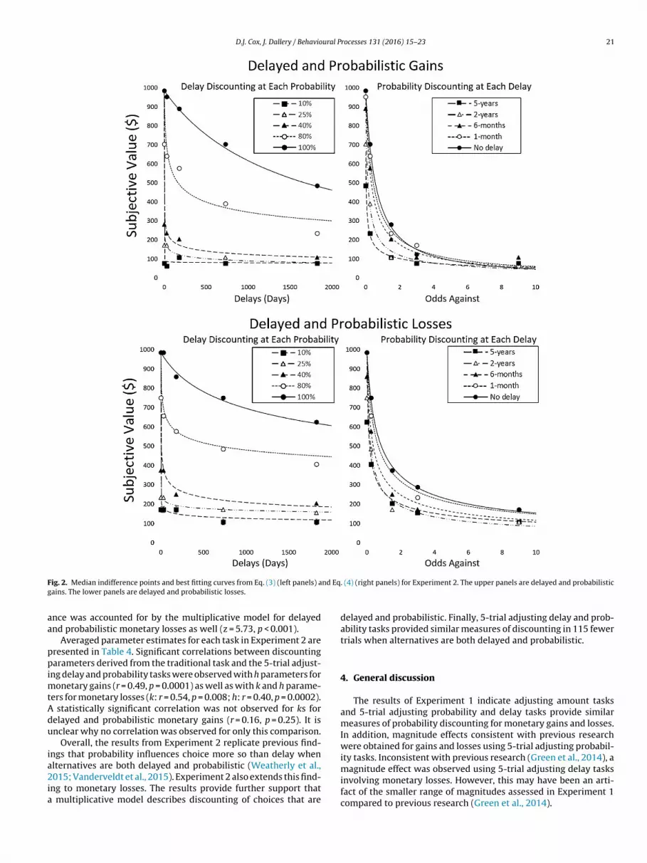

D.J. Cox, J. Dallery / Behavioural Processes 131 (2016) 15–23 21

F nd Eqg

aa

ppimtAdu

ia2ia

ig. 2. Median indifference points and best fitting curves from Eq. (3) (left panels) aains. The lower panels are delayed and probabilistic losses.

nce was accounted for by the multiplicative model for delayednd probabilistic monetary losses as well (z = 5.73, p < 0.001).

Averaged parameter estimates for each task in Experiment 2 areresented in Table 4. Significant correlations between discountingarameters derived from the traditional task and the 5-trial adjust-

ng delay and probability tasks were observed with h parameters foronetary gains (r = 0.49, p = 0.0001) as well as with k and h parame-

ers for monetary losses (k: r = 0.54, p = 0.008; h: r = 0.40, p = 0.0002). statistically significant correlation was not observed for ks forelayed and probabilistic monetary gains (r = 0.16, p = 0.25). It isnclear why no correlation was observed for only this comparison.

Overall, the results from Experiment 2 replicate previous find-

ngs that probability influences choice more so than delay whenlternatives are both delayed and probabilistic (Weatherly et al.,015; Vanderveldt et al., 2015). Experiment 2 also extends this find-

ng to monetary losses. The results provide further support that multiplicative model describes discounting of choices that are

. (4) (right panels) for Experiment 2. The upper panels are delayed and probabilistic

delayed and probabilistic. Finally, 5-trial adjusting delay and prob-ability tasks provided similar measures of discounting in 115 fewertrials when alternatives are both delayed and probabilistic.

4. General discussion

The results of Experiment 1 indicate adjusting amount tasksand 5-trial adjusting probability and delay tasks provide similarmeasures of probability discounting for monetary gains and losses.In addition, magnitude effects consistent with previous researchwere obtained for gains and losses using 5-trial adjusting probabil-

ity tasks. Inconsistent with previous research (Green et al., 2014), amagnitude effect was observed using 5-trial adjusting delay tasksinvolving monetary losses. However, this may have been an arti-fact of the smaller range of magnitudes assessed in Experiment 1compared to previous research (Green et al., 2014).

22 D.J. Cox, J. Dallery / Behavioural Processes 131 (2016) 15–23

Fig. 3. Median indifference points and best fitting curves from Eq. (6) (left panels) and Eq. (5) (right panels) for Experiment 2. The upper panels are delayed and probabilisticgains. The lower panels are delayed and probabilistic losses.

Table 4Mean and 95% confidence interval of discount parameters for each task. Pearson correlations for comparison between discounting tasks.

Task Mean k or h (95% CI) Pearson Correlation

Delayed & ProbabilisticGains

Adjusting Amount $1000 k 0.04 (0.03) 0.165-Trial Adjusting Delay $1000 k 2.93 (1.98)Adjusting Amount $1000 h 3.27 (0.66) 0.49***

5-Trial Adjusting Delay $1000 h 2.72 (0.52)Delayed & ProbabilisticLosses

Adjusting Amount $1000 k 0.001 (0.21) 0.54**

5-Trial Adjusting Delay $1000 k 0.002 (0.001)Adjusting Amount $1000 h 1.04 (0.21) 0.40***

5-Trial Adjusting Delay $1000 h 1.01 (0.21)

A*

sfcadbVopc

sterisks indicate a significant difference between tasks.p < 0.05.** p < 0.01.

*** p < 0.001.

Experiment 2 provides novel evidence that probability is morealient than delay for monetary losses, and it replicates this findingor monetary gains (Vanderveldt et al., 2015; Weatherly et al., 2015;f. Bialaszek et al., 2015). That is, when outcomes were both delayednd probabilistic and the probability of an outcome decreased,elay discounting became nearly flat. In contrast, rate of proba-

ility discounting remained steep across all delays. As reported byanderveldt et al. (2015), it is possible that the increased saliencef probability was an artifact of the range of amounts, delays, androbabilities assessed. Vanderveldt et al. (2015) suggested that oneould test these hypotheses by using a range of delays and prob-

abilities where the decrease in subjective value of an immediatereward at the lowest probability equals the decrease in subjectivevalue of a certain reward at the longest delay. Evidence would beprovided for the former hypothesis if probability continued to havea greater effect under this arrangement.

Several researchers have suggested that there are three types

of discounting: discounting of delayed gains, discounting of proba-bilistic gains, and discounting of losses (Green et al., 2014). Supportfor this position comes from the differential influence of amount onthree types of discounting. Experiment 1 provides further supportthat discounting of probabilistic gains and discounting of losses are

ural P

dottadampop2tanwi

prtoadoiolliatwdtp

5

tpoamkWwdt1ctmfa

A

atstm

Yi, R., Bickel, W.K., 2005. Representation of odds in terms of frequencies reducesprobability discounting. Psycholo. Rec. 55, 577–593.

Yi, R., Gatchalian, K.M., Bickel, W.K., 2006. Discounting of past outcomes. Exp. Clin.

D.J. Cox, J. Dallery / Behavio

istinct: increasing the magnitude resulted in steeper discountingf probabilistic gains but no change in discounting of probabilis-ic losses. Similarly, humans tend to discount gains more steeplyhan losses regardless of whether the outcome is delayed or prob-bilistic (e.g., Mitchell and Wilson, 2010). In Experiment 1, steeperiscounting of probabilistic gains was observed compared to prob-bilistic losses. In Experiment 2, gains continued to be discountedore steeply than losses when the choices were both delayed and

robabilistic. In contrast to gain/loss patterns, the effects of amountn discounting become minimal when choices are both delayed androbabilistic (Blackburn and El-Deredy, 2013; Vanderveldt et al.,015; Yi et al., 2006). Five-trial adjusting delay and probabilityasks could allow researchers to examine further these patternscross delayed, probabilistic, and delayed and probabilistic alter-atives using a within-subject study design. The resulting dataould help researchers understand whether different “impulsiv-

ties” exist even for complex choices.Future research could focus on assessing the influence of multi-

le outcomes on choices. that are delayed and probabilistic. Initialesearch could extend these tasks by adding a second outcome ofhe same commodity. For example, researchers could assess ratef delay and probability discounting of some monetary amount as

function of a second monetary outcome that occurs at varyingelays, probabilities, and amounts. Research could also assess vari-us combinations of gains and losses across the two outcomes. That

s, how does one delayed and probabilistic gain influence the valuef a second delayed and probabilistic gain? Relatedly, how does a

oss influence a gain, a gain influence a loss, and a loss influence aoss when both outcomes occur at some delay and some probabil-ty? Future research could also focus across specific commoditiess well as across consumable versus non-consumable commodi-ies. Many day-to-day choices involve more than one outcome, eachith some probability of occurrence, at differing delays, and across

ifferent commodities. The comparisons would allow researcherso test and refine quantitative models that describe choice in com-lex settings.

. Conclusion

These experiments extended research on 5-trial adjusting delayasks (Koffarnus and Bickel, 2014) from delayed monetary gains torobability discounting of monetary gains, probability discountingf monetary losses, delay discounting of monetary losses, delayednd probabilistic monetary gains, and delayed and probabilisticonetary losses. The 5-trial adjusting tasks resulted in hs and

s that correlated with hs and ks from adjusting amount tasks.e also found magnitude effects that were generally consistentith previous literature. For scenarios involving choices that were

elayed and probabilistic, 5-trial adjusting delay and probabilityasks resulted in estimation of h and k discounting parameters in15 fewer trials than an adjusting amount task. These parametersorrelated with those from adjusting amount tasks with the excep-ion of ks for delayed and probabilistic gains. The multiplicative

odel of discounting (Vanderveldt et al., 2015) described choiceor both gains and losses that were delayed and probabilistic. Delaynd probability therefore interact to influence the value of money.

cknowledgements:

The authors thank Brantley Jarvis, Philip Erb, Sarah Martner,

nd Triton Ong for their numerous comments and helpful advicehroughout the completion of this research and on previous ver-ions of this manuscript. The authors also thank the reviewers forheir insightful and very helpful feedback which strengthened the

anuscript considerably.

rocesses 131 (2016) 15–23 23

References

Bialaszek, W., Gaik, M., McGoun, E., Zielonka, P., 2015. Impulsive people have acompulsion for immediate gratification −certain or uncertain. Front. Psychol.6, 515.

Bickel, W.K., Yi, R., Kowal, B.P., Gatchalian, K.M., 2008. Cigarette smokers discountpast and future rewards symmetrically and more than controls: is discountinga measure of impulsivity? Drug Alcohol Depend. 96, 256–262.

Blackburn, M., El-Deredy, W., 2013. The future is risky: discounting of delayed anduncertain outcomes. Behav. Processes 94, 9–18.

Bruce, J.M., Bruce, A.S., Catley, D., Lynch, S., Goggin, K., Reed, D., Lim, S.L., Strober, L.,Glusman, M., Ness, A.R., Jarmolowicz, D.P., 2015. Being kind to your future self:probability discounting of health decision-making. Ann. Behav. Med., http://dx.doi.org/10.1007/s12160-015-9754-8 (epub ahead of print).

Du, W., Green, L., Myerson, J., 2002. Cross-cultural comparisons of discountingdelayed and probabilistic rewards. Psychol. Rec. 52, 479–492.

Estle, S.J., Green, L., Myerson, J., Holt, D.D., 2006. Differential effects of amount ontemporal and probability discounting of gains and losses. Mem. Cognit. 34,914–928.

Estle, S.J., Green, L., Myerson, J., Holt, D.D., 2007. Discounting of monetary anddirectly consumable rewards. Psychol. Sci. 18, 58–63.

Green, L., Fry, A.F., Myerson, J., 1994. Discounting of delayed rewards: a life-spancomparison. Psychol. Sci. 5, 33–36.

Green, L., Myerson, J., McFadden, E., 1997. Rate of temporal discounting decreaseswith amount of reward. Mem. Cognit. 5, 715–723.

Green, L., Myerson, J., Ostaszewski, P., 1999. Amount of reward has opposite effectson the discounting of delayed and probabilistic-c outcomes. J. Exp. Psychol:Learn. Mem. Cognit. 25, 418–427.

Green, L., Myerson, J., Oliveira, L., Chang, S.E., 2014. Discounting of delayed andprobabilistic losses over a wide range of amounts. J. Exp. Anal. Behav. 101,186–200.

Jimura, K., Myerson, J., Hilgard, J., Braver, T.S., Green, L., 2009. Are people reallymore patient than other animals? Evidence from human discounting of realliquid rewards. Psychono. Bull. Rev. 16, 1071–1075.

Johnson, M.W., Bickel, W.K., 2008. An algorithm for identifying nonsystematicdelay-discounting data. Exp. Clin. Psychopharmacol. 16, 264–274.

Koffarnus, M.N., Bickel, W.K., 2014. A 5-trial adjusting delay discounting task:accurate discount rates in less than one minute. Exp. Clin. Pharmacol. 22,222–228.

Magen, E., Dweck, C.S., Gross, J.J., 2008. The hidden-zero effect: representing asingle choice as an extended sequence reduces impulsive choice. Psychol. Sci.19, 648–649.

Mazur, J.E., 1987. An adjusting procedure for studying delayed reinforcement. In:Commons, M.L., Mazur, J.E., Nevin, J.A., Rachlin, H. (Eds.), Quantitative Analysesof Behavior: Vol. 5. The Effect of Delay and of Intervening Events onReinforcement Value. Erlbaum, Hillsdale, NJ, pp. 55–73.

McKerchar, T.L., Renda, C.R., 2012. Delay and probability discounting in humans:an overview. Psychol. Rec. 62, 817–834.

McKerchar, T.L., Green, L., Myerson, J., Pickford, T.S., Hill, J.C., Stout, S.C., 2009. Acomparison of four models of delay discounting in humans. Behav. Processes81, 256–259.

Mitchell, S.H., Wilson, V.B., 2010. The subjective value of delayed and probabilisticoutcomes: outcome size matters for gains but not for losses. Behav. Processes83, 36–40.

Odum, A.L., 2011. Delay discounting: i’m a k, you’re a k. J. Exp. Anal. Behav. 96,427–439.

Radu, P.T., Yi, R., Bickel, W.K., Gross, J.J., McClure, S.M., 2011. A mechanism forreducing delay discounting by altering temporal attention. J. Exp. Anal. Behav.96, 363–385.

Ritschel, F., King, J.A., Geisler, D., Flohr, L., Neidel, F., Boehm, I., Seidel, M., Zwipp, J.,Ripke, S., Smolka, M.N., Roessner, V., Ehrlich, S., 2015. Temporal delaydiscounting in acutel ill and weight-recovered patients with anorexia nervosa.Psychol. Med., http://dx.doi.org/10.1017/S0033291714002311 (epub ahead ofprint).

Vanderveldt, A., Green, L., Myerson, J., 2015. Discounting of monetary rewards thatare both delayed and probabilistic: delay and probability combinemultiplicatively, not additively. J. Exp. Psychol. Learn. Mem. Cognit. 41,148–162.

Vanderveldt, A., Oliveira, L., Green, L., 2016. Delay discounting: pigeon, rat, human– Does it matter? J. Exp. Psychol: Anim. Learn. Cognit., Advance onlinepublication.

Weatherly, J.N., Petros, T.V., J/nsd/ttir, H.L., Derenne, A., Miller, J.C., 2015.Probability alters delay discounting: but delay does not alter probabilitydiscounting. Psychol. Rec. 65, 267–275.

White, T.J., Redner, R., Skelly, J.M., Higgins, S.T., 2015. Examination of arecommended algorithm for eliminating nonsystematic delay discountingresponse sets. Drug Alcohol Depend. 154, 300–303.

Psychopharmacol. 14, 311–317.Yoon, J.H., Higgins, S.T., 2008. Turning k on its head: comments on use of an ED50

in delay discounting research. Drug Alcohol Depend. 95, 169–172.