1
Effects of selection for resistance to Sesamia nonagrioides on maize yield, 1
performance and stability under infestation with Sesamia nonagrioides and 2
Ostrinia nubilalis in Spain 3
4
G. Sandoya1; R.A. Malvar1, R. Santiago, A. Alvarez2, P. Revilla1, A. Butrón1* 5
6
1 Misión Biológica de Galicia, CSIC. Apartado 28, 36080 Pontevedra, Spain. 7
2 Estación Experimental de Aula Dei, CSIC. Apartado 202, 50080 Zaragoza, Spain. 8
9
* Corresponding mailing address: Ana Butrón, Misión Biológica de Galicia, Apdo. 28, 10
36080. Pontevedra, Spain, E-mail: [email protected], Telephone: 34986854800, 11
Fax number: 34986 841362 12
13
Abbreviations: 14
E: Environmental main effects 15
G: Genotype main effects 16
GE: Genotype environment interaction 17
GGE: G plus GE interaction 18
SREG: Sites Regression Model 19
MCB: Mediterranean Corn Borer 20
ECB: European Corn Borer 21
2
Abstract. A selection program to improve resistance to the Mediterranean corn borer 1
(MCB, Sesamia nonagrioides Lef) while maintaining yield was carried out in a maize 2
synthetic population. The objectives of this research were to investigate if yield and 3
yield stability of the maize synthetic population named EPS12 were affected by 4
selection for MCB resistance, and to determine, which genotypic and environmental 5
covariates could explain the Genotype (G), Environment (E), and Genotype × 6
Environment (GE) effects for yield under corn borer infestation. Plants from three 7
cycles of selection and their testcrosses to three inbred testers (A639, B93, and EP42) 8
were evaluated at two locations in two years, under MCB and ECB infestations. After 9
selection EPS12 was a more stable genotype. Hybrids derived from crosses between 10
B93 and inbreds obtained from the initial cycles of selection could be recommended for 11
cultivation in northern Spain. The yield of crosses between cycles of selection and 12
testers increased with when there were fewer days with mean temperatures > 25 ºC and 13
higher mean maximum temperatures. Differences for yield among these genotypes were 14
mostly explained by resistance to corn borer attack. In general, among EPS12 derived 15
materials, genetic characteristics that contribute to increased grain yield were also 16
responsible for increased abiotic stress tolerance. 17
18
Key words: maize, yield, stability, GGE interaction, Sesamia nonagrioides, Ostrinia 19
nubilalis 20
3
Introduction 1
2
Insect herbivores cause high yield losses in crops. In maize (Zea mays L.), yield losses 3
due to insect pest attacks are in average 16% (Oerke, 2006). In southern Europe, there 4
are two species of corn borer which attack maize, namely European corn borer (ECB), 5
Ostrinia nubilalis Hbn (Lepidoptera: Crambidae), and Mediterranean corn borer 6
(MCB), Sesamia nonagrioides Lef, (Lepidoptera: Noctuidae) (Cordero et al., 1998; 7
Velasco et al., 2007). In Spain, MCB seems to be the most damaging pest of maize 8
(Castañera, 1986), specifically, in northwestern Spain where periodic samplings of 9
maize indicated that there were 1.2 larvae of MCB and 0.12 larvae of ECB per plant 10
(Cordero et al., 1998). Larvae of the second and subsequent generations of these borers 11
attack maize near flowering time by entering into the stem, causing stem-tunneling that 12
weakens plants, provokes lodging and reduces yield. 13
In Spain, maize is produced in two well-differentiated regions - northern Spain 14
and inland Spain. Northern Spain has an Atlantic climate with mild temperatures and 15
high rainfall, whereas inland Spain has a dry climate, low rainfall and warmer 16
temperatures during the growing season. Mediterranean corn borer is more abundant in 17
coastal northwestern Spain, whereas ECB and MCB populations are equally important 18
in central Spain (Malvar et al., 1993; Cordero et al., 1998; Velasco et al., 2007). 19
Because insect damage impacts maize yield, it is important to select genotypes that 20
perform stably across environments with different climates and borer species 21
populations. Identifying superior cultivars for the target region(s) should be done by 22
conducting regional performance trials. Superior cultivar performance in a particular 23
environment is a combination of environment main effects (E), genotype main effects 24
(G), and genotype × environment interaction effects (GE). When high levels of 25

4
variation are due to environmental factors, use of the Sites Regression (SREG) method 1
is recommended (Crossa & Cornelius, 1997). This multiplicative method considers G 2
and GE effects simultaneously (Yan et al., 2000) and has been used by several authors 3
to study yield potential and stability (Malvar et al., 2005; Castillo et al., 2005; Fan et 4
al., 2007; Setimela et al., 2007). 5
In addition, the Factorial Regression approach can be used to obtain a biological 6
explanation of genotype (G) and environmental (E) main effects, and GE interaction 7
effects (Denis, 1988; Vargas et al., 1999). Epinat-Le Signor et al. (2001) studied the 8
grain yield stability of 132 hybrids across 12 years and different locations in France and 9
they determined that most of the GE variability was due to differences for earliness and 10
yield limiting factors. Malvar et al. (2005) studied the performance of crosses among 11
French and Spanish populations across eight environments, concluding that effects of G, 12
E, and GE for grain yield were mainly due to earliness, vigor effects, and/or 13
environmental factors related to cold stress. Neither genotypic covariates nor 14
environmental covariates related to resistance to stem borers and level of infestation, 15
respectively, were taken into account in these studies. 16
Butrón et al. (2004) studied G, E, and GE for yield under natural infestation by 17
S. nonagrioides and concluded that GE effects were mainly due to earliness, vigor 18
effects, and environmental factors such as average minimum temperature and 19
percentage of air humidity.. However, the study was conducted with inbreds from 20
different backgrounds evaluated under natural conditions, a situation that could preclude 21
detection of relationship between resistance and yield. In the present study, three 22
selection cycles developed by classical plant breeding that shared a common 23
background, and their crosses to testers were used. Therefore any possible 24

5
overestimation or underestimation of resistance was avoided because genotypes were 1
evaluated under artificial infestations with MCB and ECB eggs. 2
A selection program was carried out in the EPS12 maize synthetic population to 3
improve resistance to MCB while maintaining yield by using the S1 intrapopulational 4
recurrent selection method. Stem damage was reduced significantly whereas yield did 5
not significantly decrease (Sandoya et al., 2008). However, the study of the effects of 6
selection on yield and yield stability should be done together because genotype × 7
environment effects for yield could be as important as main genotype effects. This type 8
of study should address the selection cycle that is the best in terms of yield performance 9
and stability as well as resistance to insect attack. Since the final goal of maize breeding 10
is the development of better hybrids, it is important to determine the possible biological 11
causes for yield variation in the crosses of cycles of selection with testers. Therefore, the 12
objectives of this research were to investigate if yield and yield stability were affected 13
by selection for MCB resistance and to determine which genotypic and environmental 14
covariates explain the Genotype (G), Environment (E), and Genotype × Environment 15
(GE) effects for yield under corn borer infestation using crosses between selection 16
cycles with testers. 17
6
Materials and methods 1
2
The Selection Program of EPS12 maize synthetic population 3
The S1 recurrent selection program used to improve resistance of EPS12 against MCB 4
was initiated in 1993 with about 150 S1 families. In 1994, 100 S1 progenies were 5
evaluated under artificial infestation with eggs of S. nonagrioides, and the 10 lines that 6
showed the shortest stem tunnel length and yield above the mean of the 100 families 7
were selected. In 1995, selected families were recombined, and the first cycle of 8
recurrent selection EPS12(S)C1 was established in 1996, EPS12(S)C2 and EPS12(S)C3 9
were obtained in 1999 and 2002, respectively. Unfortunately, EPS12(S)C1 seeds were 10
accidentally mixed with seeds from another maize synthetic, and they could not be 11
included in the present study. Nevertheless, the selection process was not affected 12
because S1 families were obtained from EPS12(S)C1-Syn1 before recombination to 13
obtain EPS12(S)C1. 14
15
Plant material and methods 16
Twelve genotypes were used to study the changes in stability due to selection while nine 17
of these genotypes were used to find the relationships between genotypic and 18
environmental covariates and yield. These genotypes were the three cycles of selection 19
per se derived from EPS12 (used only to study changes in stability), and their 20
testcrosses with three different inbred testers (EP42, B93 and A639 representing the 21
humid Spain, the Lancaster and the Reid heterotic groups, respectively). Evaluations 22
were made in two different types of experiments, one infested with MCB eggs and 23
another one with ECB eggs, at two locations in two years, resulting in eight different 24
trials. 25
7
In each trial, the twelve populations studied were arranged in a randomized 1
complete block design with three replications. The experiments were conducted in two 2
well-differentiated Spanish locations: Pontevedra (42º24’ N, 8º38’ W, 20 m above sea 3
level), and Zaragoza (41º 44’ N, 0º 47’ W, 230 m above sea level) in two years - 2003 4
and 2004. In Pontevedra, each experimental plot was hand-planted and consisted of two 5
rows spaced 0.80 m. apart with 25 two-plant hills spaced 0.21 m. apart. Plots were 6
overplanted and thinned to leave 1 plant per hill, the final density being ≈ 60,000 plants 7
ha-1. In Zaragoza, plots were machine-planted and consisted of two rows spaced 0.75 m 8
apart with 27 two-plant hills spaced 0.18 m apart. Plots were overplanted and thinned, 9
and the final density was ≈ 74,000 plants ha-1. In each location and year, trials infested 10
with MCB and ECB eggs were adjacent. 11
At flowering, artificial infestations with MCB eggs were carried out in ten 12
adjacent and competitive plants per plot. Infestations were made by laying a mass of 13
about 40-50 eggs between the main ear and the stem, as described by Butrón et al. 14
(1998). The MCB rearing method used was described by Eizaguirre & Albajes (1992), 15
the rearing methodology was carried out in the insect rearing laboratory at the Mision 16
Biologica de Galicia (Pontevedra – Spain). ECB eggs were supplied by the Institute 17
National de la Recherche Agronomique (France). 18
19
Traits recorded 20
The traits recorded were as follows: tunnel length (at harvest, stalks of ten infested 21
plants per plot were longitudinally split to measure the total length in cm per plant of 22
tunnels made by borers), percentage of stem damaged (estimated as tunnel length 23
divided by plant height), yield (expressed as Mg ha-1 at 140 g H2O kg-1), visual ratings 24
for ear, cob, shank, grain, and husk damages (on a 9 point subjective scale determined 25

8
as follows: 1 = > 90% damaged, 2 = 81 to 90% damaged, 3 = 71 to 80% damaged, 4 = 1
61 to 70% damaged, 5 = 41 to 60% damaged, 6 = 31 to 40% damaged, 7 = 21 to 30% 2
damaged, 8 = 1 to 20% damaged, and 9 = 0%), early vigor (at approximately five-leaf 3
stage, on a subjective scale from 1= the least vigorous to 9= the most vigorous plants], 4
plant and ear heights (recorded on ten competitive plants, length from the surface to the 5
node of the male inflorescence and to the insertion of the main ear, respectively), days 6
to pollen shedding (days from planting to 50% of plants shedding pollen), days to 7
silking (days from planting to 50% of plants showing silks), ear-row number, ear length 8
(cm), and 100-kernel weight (g). 9
Tunnel length and visual ratings for ear, cob, shank, grain and husk damages 10
were recorded in the infested plants, whereas, plant and ear height, ear-row number, ear 11
length, and 100-kernel weight were taken in ten randomly-chosen plants per plot. Days 12
to pollen shedding and to silking as well as yield were recorded on per plot basis. All 13
traits except grain yield were considered genotypic covariates. 14
To obtain a biological explanation for the E and GE effects, some environmental 15
variables defining environmental conditions during maize growth period were recorded. 16
These included number of surviving larvae of MCB and ECB per stem and ear (values 17
recorded in the ten infested plants), stem tunnel length estimated in cm in each 18
environment, daily mean minimum, maximum and daily mean temperatures in ºC, 19
rainfall in mm, percentage of air humidity, and the number of days with daily mean 20
temperatures > 30 ºC, > 25 ºC, <15 ºC, and <10 ºC. Meteorological data were recorded 21
by stations that were < 500 m from trials. 22
23
Statistical Analysis 24
SREG Method 25

9
1
Each environment was defined as the combination of a year, a location, and infestation 2
with a particular borer species; resulting in eight different environments under study. 3
The SREG method was used to study the GGE component of yield variability among 4
cycles of selection and crosses of cycles to testers. 5
The fixed-effect two-way model for the analysis of multienvironmental genotype 6
trials by the SREG model is as follows (Cornelius et al., 1996; Crossa & Cornelius, 7
1997): 8
Yij = μ + j + *in *
jn 9
10
where k goes from 1 to r, with r = number of principal components (PCs) required to 11
approximate the original data. Yij is the mean grain yield of genotype i in the 12
environment j; μ is the mean value, βj is the environmental main effect and, ξ*in and η*jn 13
are the ith genotype and the jth environmental scores on the kth PC, respectively. The 14
analysis was performed with plot data as is shown by the degrees of freedom. SREG 15
analysis was computed by a SAS (SAS Institute, 2007) program which was developed 16
by Burgueño & Crossa (2003). 17
With the SREG method, PC analysis is made on residuals of an additive model 18
with environmental effects being the only main ones. Therefore, the term *in *
jn 19
contains the variation due to G and GE interactions. A two-dimensional biplot (Gabriel, 20
1971) called GGE biplot (G plus GE interaction) of the first two PCs was used to 21
display the genotypes and the environments simultaneously (Yan et al., 2000). Each 22
genotype and environment was defined by its respective score on the two PCs. The 23
which-won-where view method of the GGE biplot (Yan et al., 2000) was also used to 24
predict which genotype is particularly favored in each environment. 25
26
10
Factorial regression method 1
2
For this analysis, each environment was considered as the combination of a location and 3
a year because all environmental covariates detected as significant by the stepwise 4
method were indeed meteorological variables that were common to both MCB and ECB 5
infested trials. Therefore only four environments were taken into account. 6
Cycles per se were not included in this analysis. As cycles and cycles testcrossed 7
to testers have different levels of heterosis, the inclusion of both types of genotypes will 8
presumably bring information about those genotypic covariables that better distinguish 9
between cycles and crosses. However, our goal is to obtain a biological explanation on 10
G and GE variability among crosses because they represent different heterotic patterns. 11
The general formula for a factorial regression model with K genotypic and H 12
environmental covariates is (Denis, 1980; Vargas et al., 1999): 13
Yij = μ + [Σk.Gik + i] + [Σh.jh + j] + [ΣGik.kh.jh + Σ’ih.jh+ Σ’jk.Gik + ij] 14
where k and h are the regression coefficients of genotypic Gik, and environmental 15
covariates jh, respectively; i and j are the residuals of genotype and environmental 16
main effects respectively, respectively; kh is the regression coefficient of the cross-17
product of covariates Gik and jh; ’ih and ’jk are the genotype i and environment j 18
specific regression coefficients of genotypic covariate Gik and environmental covariate 19
jh, respectively; and ij is the residual genotype × environment interaction effect. All 20
parameters of this model were considered fixed effects. The covariates and their order in 21
the factorial regression model for grain yield were obtained by performing a stepwise 22
regression on genotypic covariates and a second stepwise regression on environmental 23
covariates (Denis, 1988). After standardization of covariates, factorial regression 24
analyses were performed by the software INTERA (Decoux & Denis, 1991). All factors 25

11
were tested against residual experimental error. 1

12
Results 1
2
SREG 3
4
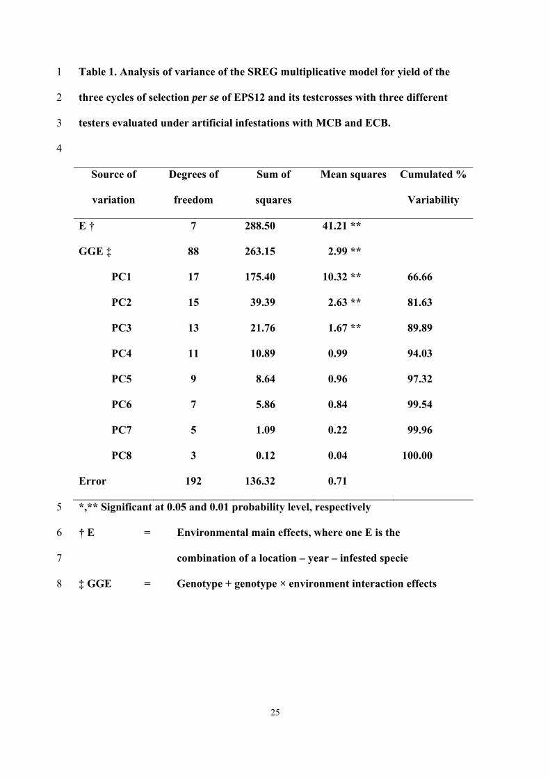
The SREG analysis showed that E and GGE variation for yield were highly significant 5
(Table 1). The most important sum of squares for grain yield under infestation was E, 6
which explained 42% of the total variation for yield while GGE explained 38%. 51% of 7
the proportion explained by GGE was accounted for by GE while the remaining 49% 8
was due to G effects. 9
From the eight principal components (PCs) obtained after singular value 10
decomposition of location-centered yield, the first three PC’s were highly significant 11
and explained 89.89% of GGE variation; the remaining components were not 12
significant. The first two PCs of the SREG explained 81.63% of GGE variation (Table 13
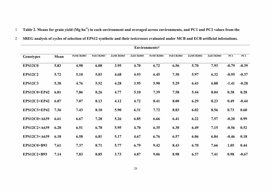
1). Mean values for grain yield were significantly higher in Pontevedra than in 14
Zaragoza, and yield values in 2003 were significantly lower than in 2004 (Data not 15
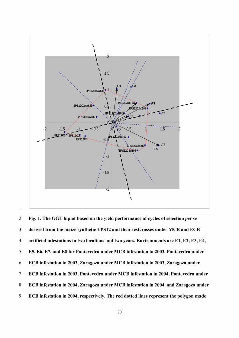
shown). In general, the three cycles of selection and their testcrosses to A639 showed 16
negative values for the projections of the scores on the new abscissa exe (Fig. 1); 17
meanwhile, the highest abscissa values were presented by EPS12C0 × B93 and 18
EPS12C3 × EP42. 19
The ordinate values for the cycles of selection per se were low; but the initial 20
cycle of selection presented a higher value than the next cycles. Among testcrosses, 21
EPS12C0 × B93 and EPS12C0 × EP42 showed the lowest ordinate values. 22
According to Figure 1, the EPS12C0 × B93 would be favored compared to the 23
other genotypes in Pontevedra in 2003 under MCB and ECB infestations, and in 24
Zaragoza in 2004 under ECB infestation; meanwhile EPS12C2 × B93 showed the 25
13
highest positive interaction with Pontevedra in 2004 under MCB and ECB infestations, 1
and in Zaragoza in 2004 under MCB infestation, EPS12C3 × EP42 would be favored in 2
Zaragoza in 2003 under ECB infestation, and EPS12C0 × A639 in Zaragoza in 2003 3
under MCB infestation (Figure 1). 4
5
Factorial regression 6
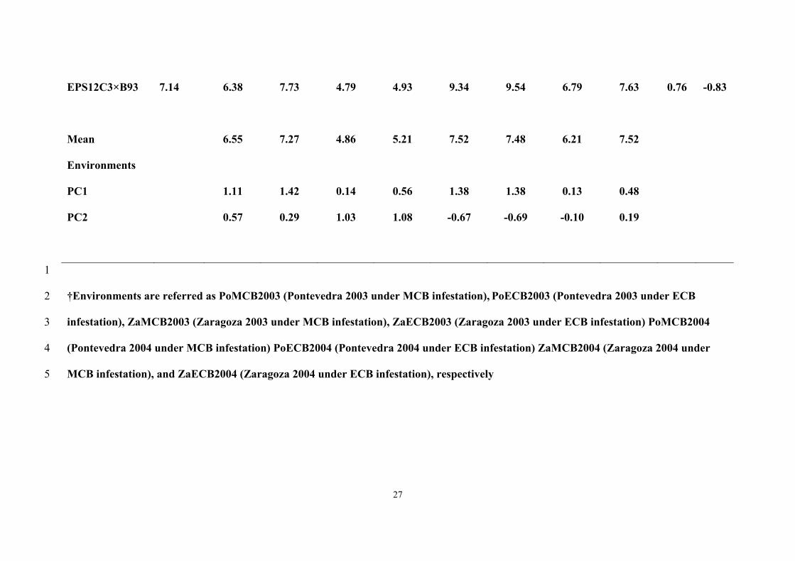
The genotypic covariates detected as significant by the stepwise method were 7
days to pollen shedding (PS), plant height (PH), ECB in the ear (ECB), tunnel length 8
(TL), stalk lodging (SL), and days to silking (S); whereas number of days with daily 9
mean temperatures > 25 ºC (TM25) and mean maximum temperature (Tmax) were 10
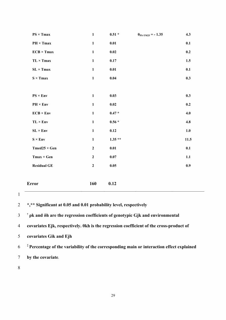
detected as significant environmental covariates (Table 3). 11
Genotypes showed highly significant variation for S and ECB, while differences 12
for PS, PH, SL, and TL were significant. Variability for PS, PH, SL, ECB, S and TL 13
explained approximately 90% of the G variation. The regression coefficients of G 14
variation for yield on PS, PH and ECB were positive (ρPS = 4.64, ρPH = 0.05, ρECB = 15
0.31, respectively) and on SL and TL were negative (ρSL = -0.20 and ρPS = -0.32, 16
respectively). 17
The environmental covariates (TM25 and Tmax ) explained almost the 100% of 18
the variation for E among testcrosses. The regression coefficients of the environmental 19
covariates were positive for Tmax (δTmax= 0.55) and negative for TM25 (δTM25= -1.61). 20
Three cross-products between genotypic covariates and the environmental 21
covariate TM25 were significant, PH × TM25 (highly significant), ECB × TM25 22
(significant) and SL ×TM25 (highly significant), and explained approximately the 65% 23
of the sum of squares for GE. The regression coefficients for the cross-products PH × 24
TM25, ECB × TM25 and SL ×TM25 were -0.58, 0.09, and 0.62, respectively. The 25

14
cross-products between the genotypic covariate PS and the environmental covariable 1
Tmax was significant and explained approximately the 4% of the sum of squares for 2
GE. The regression parameters of yield on PS × Tmax was negative (-1.35). 3
The interaction of three genotypic covariates, ECB, TL, and S, with the residual 4
environmental variation (Env) were significant for ECB and TL and highly significant 5
for S, they explained the 20% of the sum of square for the interaction. The interactions 6
of the environmental covariates (Tmax and TM25) with the residual genotype variation 7
were not significant and explained less than 1.5% of the GE variation. 8

15
Discussion 1
2
The percentages of the total sum of squares for grain yield explained by E and GGE 3
were similar to those reported by other authors, although the geographical proximity 4
among locations and genetic variability were very different across studies (Butrón et al., 5
2004; Malvar et al., 2005). In the present study, artificial infestation, necessary to 6
adequately estimate genotype resistance, could partly have homogenized the conditions 7
across environments. 8
Percentage of variation due to G was lower than that reported by Butrón et al. 9
(2004) for a set of 45 hybrids and by Malvar et al. (2005) for a diallel among 12 10
populations. Genotypes included in this study had similar genetic background because 11
all were derived from the same population, EPS12. Therefore, although genotypic 12
differences were diminished compared to other studies, the relationship between 13
stability and genotype yield performance, as well as between genotypic covariates and 14
GGE, were less biased by background differences than in previous studies. 15
The high percentage of GGE variation in the first two PCs of the SREG suggests 16
that a biplot of PC1 and PC2 adequately approximates the environment-centered data 17
(Yan et al., 2007). The PC1 reflects the mean performance plus the noncrossover GE 18
interaction if the primary effects of sites from the SREG model are all of the same sign 19
in the two dimensional biplot (Yan et al., 2000; Crossa et al., 2002). PC2 represents the 20
disproportionate yield differences across environments. 21
We used the symmetric scaling method for the biplot drawing because it has 22
intermediate properties between the genotype and the environmentally-focused scaling 23
method. This method does not show the genotypes with the largest yield at each 24
16
environment, but it does show the one particularly favored by these conditions 1
compared to the other genotypes, independent of its mean value for yield. 2
Besides, we have also used the GGE biplot recommended by Yan et al. (2001) 3
which forces the abscissas to present the genotype main effect and is, therefore, more 4
interpretable in terms of mean performance and stability (In Figure 1, the black dotted 5
lines become the x and y abscissas). Hence, new axes were obtained by using the 6
average environment, which forces the abscissa to present the genotype main effect and, 7
consequently, facilitates the interpretation of the biplot in terms of mean performance 8
and stability of the genotypes (Yan, 2002). The two-dimensional biplot showed that 9
cycles per se were grouped together as the yield worst producers. 10
Although it was not statistically significant, it was previously shown that the 11
yield performance of genotypes from the EPS12 selection cycles was negatively 12
affected by the selection process (Sandoya et al., 2008), however, stability seemed to 13
improve during selection. The higher genotype mean effect for yield was accompanied 14
by lower stability across cycles per se or crossed to A639 and EP42. That suggests that 15
higher heterosis is associated to lower stability. Nevertheless there was a positive 16
relationship between stability and heterosis among cycles of selection crossed to B93,. 17
Therefore, for the entire target region, inbreds will be preferentially obtained from the 18
initial cycle of selection in order to obtain promising hybrids, in terms of yield 19
performance and stability, when crossed to B93. Alternatively, a breeding program to 20
improve the specific combining ability between EPS12 and B93 could be performed. 21
In Pontevedra the genotypes showed a better performance for yield and less 22
cross-over interaction than in Zaragoza. This could be consequence of having multiplied 23
and improved the synthetic population from which EPS12 was released, EPS7 (Vales et 24
al., 2001), and EPS12 itself at Pontevedra for more than 20 years. Adaptation to mild 25

17
climate conditions, such as those present in northern Spain, has probably been enhanced 1
in parallel to the intended increases for yield and resistance to MCB attack. Therefore, 2
we discourage any cultivar recommendation for Central Spain because these materials, 3
although descendant from populations collected in Central Spain, no longer show 4
adaptation to those environments. These results emphasize the preliminary nature of our 5
study and reinforce the importance of choosing the target environment and performing 6
selection based on performance across locations with well differentiated climatic 7
characteristics if the target environment covers an extensive geographical region 8
(Setimela et al., 2005). Hence we will limit our recommendations to northern Spain. 9
Differences for yield between both infestation species were only significant in 10
2003 because temperatures were higher than usual, favoring pest development, 11
especially MCB, which has an African origin (Sandoya et al., 2008). The cross 12
EPS12C0 × B93 would be the best cultivar for years with exceptionally warm 13
temperatures, such as those observed in 2003, but the cross EPS12C2 × B93 would 14
perform better across years with mean temperatures more similar to the average 15
temperature of the last 25 years. Our main suggestion is to initiate a breeding program 16
in EPS12C2 in order to improve its specific combining ability with B93 under 17
infestation with MCB eggs. 18
The two regression coefficients of yield G variation on the genotypic covariates 19
plant height (PH) and ECB in the ear (ECB) were positive, indicating that taller 20
genotypes with higher presence of ECB in the ears are more productive, whereas stalk 21
lodging (SL) and tunnel length (TL), both indirect and direct consequences, 22
respectively, of corn borer attack were detrimental to yield. The effect of maturity on 23
yield was low because regression coefficients for days to pollen shedding and to silking 24
were similar in value and with opposite direction. Several authors (Argillier et al., 1994; 25

18
Epinat-Le Signor et al., 2001; Butrón et al., 2004; Malvar et al., 2005) reported that G 1
variation for grain yield was mainly due to earliness and vigor. However, in the present 2
study, all genotypes shared a common background and were infested with MCB and 3
ECB eggs to avoid any possible escape of borer attack. In this scenario, precocity 4
reduces considerably its influence on yield and, in consequence, genotypic 5
characteristics related to heterosis, such as plant height, and characteristics related to 6
resistance to borers, such as tunnel length and stem lodging, appeared as the most 7
determinant for yield. 8
The factorial regression analyses showed that yield increased when the number 9
of days with temperatures > 25 ºC (T) diminishes and mean maximum temperature 10
(Tmax) increases. Maize is a tropical crop and optimum temperatures during the 11
growing period from sowing to tassel initiation could vary between 22 and 31 ºC, 12
depending on the genotype (Ellis et al., 1992). However, maize plants under high 13
temperatures exhibit decreased leaf area index, less total biomass production, and loss 14
of grain yield (Westgate et al., 2004). Shaw (1988) suggested that, during reproductive 15
development, each 1 ºC increase in temperature above optimum (25 ºC) results in 16
reduction of 3 to 4% in grain yield. Cheik & Jones (1994) showed that kernels exposed 17
to short-term (four days) heat stress exhibited a recovery in kernel growth, but kernel 18
fresh and dry matter accumulation was severely reduced by long-term heat stress. 19
Therefore, the number of days with mean temperature higher than 25 ºC would 20
characterize heat stress conditions better than the daily maximum temperatures. In 21
addition, the development of the MCB would be favored by more days with high mean 22
temperatures because this species is a tropical moth. Once the unfavorable effects of 23
heat stress and insect pressure are removed, warmer environments, characterized by 24
higher mean maximum temperatures, would be more favorable for maize development. 25

19
The regression coefficients of yield on the cross-product between genotypic and 1
environmental covariates showed that characteristics favorable for increased yield, 2
except reduced stalk lodging, were more favorable under environments with higher 3
stress. This positive interaction between yield-related traits and environmental stress 4
explained more than 50% of variability for GE and agrees with the idea that genetic 5
characteristics that contribute to increased grain yield could also be responsible for 6
increased abiotic stress tolerance (Lee & Tollenaar, 2007). The positive SL × TM25 7
interaction suggests that there is a competition between using resources to resist insect 8
biotic stress (insect attack) and abiotic stress (heat). 9
10
Conclusions 11
Selection for corn borer resistance increased the stability of the maize synthetic 12
EPS12 under artificial infestation with MCB and ECB. A positive correspondence 13
between stability and yield performance was observed only when plants from cycles of 14
selection were crossed to B93. Therefore, for the target region of the European Atlantic 15
coast, we suggest initiating a breeding program with EPS12C2 to improve its specific 16
combining ability with B93 under infestation with MCB eggs. Yield differences among 17
these genotypes were mainly due to differences for resistance to corn borer attack; 18
while, heat stress was the most yield limiting environmental factor. In EPS12, genetic 19
characteristics that contribute to increased grain yield could also be responsible for 20
increased abiotic stress tolerance. 21
22
Acknowledgment: Thanks to Raquel Díaz and Emma Muiños for rearing insects. Also, 23
thanks to all the people who work in our farm. 24

20
G. Sandoya acknowledges three consecutive grants from: C. Iturriaga and Maria de 1
Dañobeitia Foundation, the Mediterranean Agronomic Institute of Zaragoza 2
(CIHEAM), and the Ministry of Education and Science (Spain). 3
Dr. Dawn S. Luthe for language corrections. 4
This research was also supported by the Plan Nacional I+D+I (AGL2003-00961 and 5
AGL2006-1314) and the “Excma. Deputación Provincial de Pontevedra”. 6
21
References 1
2
Argillier O., Hébert Y., Barrière Y. (1994) Statistical analysis and interpretation of line 3
environment interaction for biomass yield in maize. Agronomie, 14, 661-672. 4
Burgueño J., Crossa J. (2003) Graphing GE and GGE biplots. In. Handbook of formulas 5
and software for geneticist and breeders. Manjit S Kang (ed.) Chapter 18. The 6
Haworth Press Inc. New York. 7
Butrón A., Malvar R.A., Velasco P., Revilla P., Ordás A. (1998) Defense mechanisms 8
of maize against pink stem borer. Crop Science, 38, 1159-1163. 9
Butrón, A., P. Velasco, A. Ordás, and R.A. Malvar (2004) Yield evaluation of maize 10
cultivars across environments with different levels of pink stem borer. Crop 11
Science, 44, 741-747. 12
Castañera P (1986) Plagas del Maíz. IV. Jornadas Técnicas Sobre El Maíz, Lérida. 13
Plagas, pp. 1–24. Ministerio de Agricultura Pesca y Alimentación, Madrid, Spain. 14
Castillo HD, Sanchez FR, Valdes MHR, Garduno DS, Zambrano GM, Cadena RC, 15
Cardenas JDF (2005) Yield potential and stability of germplasm combinations 16
developed among maize groups. Revista de Fitotecnia Mexicana, 28, 135-143. 17
Cheik N., Jones R.J. (1994) Disruption of maize kernel growth and development by heat 18
stress. Plant Physiology, 106, 45 – 51. 19
Cordero A., Malvar R.A., Butrón A., Velasco P., Revilla P., Ordás A. (1998) 20
Population dynamics and life-cycle of corn borers in South Atlantic European 21
coast (Lepidoptera, Noctuidae, Pyralidae). Maydica, 43,5-12. 22
Cornelius P.L., Crossa J., Seyedsader M.S. (1996) Statistical test and estimators of 23
multiplicative models for genotype-by-environment interaction. Pp. 199-234. In 24
M.S. Kang and H.G. Cauch (eds.) Genotype-by-environment interaction. CRC 25
22
Press, Boca Raton, Florida. 1
Crossa J., Cornelius P.L. (1997) Sites regression and shifted multiplicative model 2
clustering of cultivar trial sites under heterogeneity of error variances. Crop 3
Science, 37, 406-415. 4
Crossa J., Cornelius P.L., W. Yan (2002) Biplots of linear-bilinear models for studying 5
crossover genotype environment interaction. Crop Sci. 42:619-633. 6
Decoux G., Denis J.B. (1991) INTERA. Logiciels pour l’interprétation statistique de 7
l’interaction entre deux facteurs. Laboratoire de Biométrie, INRA, Route de 8
Saint-Cyr F78026, Versailles, France. 9
Denis J.B. (1980) Analyse de régression factorielle. Biom. Praxim. 20:1-34. 10
Denis J.B. (1988). Two way analysis using covariates. Statistics, 19, 123-132. 11
Eizaguirre M., Albajes R. (1992). Diapause induction in the stem corn borer, Sesamia 12
nonagrioides (Lepidoptera: Noctuidae). Entomologia Generalis, 17, 277-283. 13
Ellis R.H., Summerfield R.J., Edmeades G.O., Roberts E.H. (1992) Photoperiod, 14
temperature, and the interval from sowing to tassel initiation in diverse cultivars 15
of maize. Crop Science, 32, 1225-1232. 16
Epinat-Le Signor C., Dousse S., Lorgeou J. Denis J.B., Bonhomme R., Carolo P., 17
Charcosset A. (2001) Interpretation of genotype environment interactions for 18
early maize hybrids over 12 years. Crop Science, 41, 663-669. 19
Fan X.M., Kang M.S., Chen H.M., Zhang Y.D., Tan J., Xu C.X. (2007) Yield stability 20
of maize hybrids evaluated in multi-environment trials in Yunnan, China. 21
Agronomy Journal, 99,220-228. 22
Gabriel K.R (1971) The biplot graphic display of matrices with application to principal 23
component analysis. Biometrika, 58, 453-467. 24
Lee E.A., Tollenaar M. (2007) Physiological basis of successful breeding strategies for 25
23
maize grain yield. Crop Science, 47, S-202-215S. 1
Malvar R.A., Cartea M.E., Revilla P., Ordás A., Alvarez A., Mansilla J.P. (1993) 2
Sources of resistance to pink stem borer and European corn borer in maize. 3
Maydica, 38, 313-319. 4
Malvar R.A., Revilla P., Butrón A,, Gouesnard B., Boyat A., Soengas P., Alvarez A., 5
Ordás A. (2005) Performance of crosses among French and Spanish maize 6
populations across environments. Crop Science, 45, 1052-1057. 7
Oerke, E.C. (2006) Crop losses to pests. Journal of Agricultural Sciences 144, 31-43. 8
Sandoya G., Butrón A., Alvarez A., Ordás A., Malvar R.A. (2008) Direct response of a 9
maize synthetic to recurrent selection for resistance to stem borers. Crop 10
Science, 48, 113-118. 11
Setimela P.S., Chilatu Z., Jonazi J., Mambo A., Hodson D., Bänziger M. (2005) 12
Environmental classification of maize testing sites in the SADC region and its 13
implication for collaborative maize breeding strategies in the subcontinent. 14
Euphytica, 145,123-132. 15
Setimela P.S., Vivek B., Bänziger M., Crossa J., Maideni F. (2007) Evaluation of early 16
to medium maturing open pollinated maize varieties in SADC region using GGE 17
biplot based on the SREG model. Field Crops Research, 103, 161-169. 18
SAS (2007) The SAS System. SAS Online Doc. HTML Format Version eight. SAS 19
Institute Inc., Cary, North Carolina. 20
Shaw R.H. (1988) Climate requirement. Pp: 609 – 638. In: G.F. Sprague and J.W. 21
Dudley (eds.) Corn and corn improvement. 3rd ed. ASA, Madison. Wisconsin, 22
USA. 23
Vargas M., Crossa J., Van Eeuwijk F.A., Ramírez M., Sayre K. (1999) Using partial 24
least squares regression, factorial regression, and AMMI models for interpreting 25
24
Genotype Environment interaction. Crop Science, 39, 955 – 967. 1
Vales M.I., Malvar R.A., Revilla P., Ordás A. (2001) Recurrent selection for grain yield 2
in two Spanish maize synthetic populations. Crop Science, 41, 15–19. 3
Velasco P., Revilla P., Monetti L., Butrón A., Ordás A., Malvar R.A. (2007) Corn 4
borers in northwestern Spain. Population dynamics and distribution. Maydica, 5
52, 195 – 204. 6
Westgate M.E., Otegui M.E., Andrade F.H. (2004) Physiology of the corn plant. In. 7
C.W. Smith, J. Betrán, E.C.A. Runge (eds.) Corn: origin, history, technology, 8
and production. USA. 9
Yan, W. (2002) Singular-value partitioning in biplot analysis of multienvironment trial 10
data. Agronomy Journal, 94, 990-996. 11
Yan, W., Cornelius P.L., Crossa J., Hunt L.A. (2001) Two types of GGE biplots for 12
analyzing multi-environment trial data. Crop Science, 41, 656 – 663. 13
Yan, W, Hunt L.A., Sheng Q., Szlavnics Z. (2000) Cultivar evaluation and mega-14
environment investigation based on the GGE biplot. Crop Science, 40, 597-605. 15
Yan, W., Kang M.S., Ma B., Woods S., Cornellius P.L. (2007) GGE biplot vs. AMMI 16
analysis of genotype-by-environment data. Crop Science, 47, 643–655. 17
18
25
Table 1. Analysis of variance of the SREG multiplicative model for yield of the 1
three cycles of selection per se of EPS12 and its testcrosses with three different 2
testers evaluated under artificial infestations with MCB and ECB. 3
4
Source of
variation
Degrees of
freedom
Sum of
squares
Mean squares Cumulated %
Variability
E † 7 288.50 41.21 **
GGE ‡ 88 263.15 2.99 **
PC1 17 175.40 10.32 ** 66.66
PC2 15 39.39 2.63 ** 81.63
PC3 13 21.76 1.67 ** 89.89
PC4 11 10.89 0.99 94.03
PC5 9 8.64 0.96 97.32
PC6 7 5.86 0.84 99.54
PC7 5 1.09 0.22 99.96
PC8 3 0.12 0.04 100.00
Error 192 136.32 0.71
*,** Significant at 0.05 and 0.01 probability level, respectively 5
† E = Environmental main effects, where one E is the 6
combination of a location – year – infested specie 7
‡ GGE = Genotype + genotype × environment interaction effects 8
26
Table 2. Means for grain yield (Mg ha-1) in each environment and averaged across environments, and PC1 and PC2 values from the 1
SREG analysis of cycles of selection of EPS12 synthetic and their testcrosses evaluated under MCB and ECB artificial infestations. 2
Environments†
Genotypes Mean PoMCB2003 PoECB2003 ZaMCB2003 ZaECB2003 PoMCB2004 PoECB2004 ZaMCB2004 ZaECB2004 PC1 PC2
EPS12C0 5.83 4.98 6.08 3.95 4.70 6.72 6.56 5.70 7.93 -0.79 -0.39
EPS12C2 5.72 5.10 5.03 4.68 4.93 6.45 7.30 5.97 6.32 -0.95 -0.37
EPS12C3 5.38 4.76 5.52 4.28 3.95 5.90 5.29 6.43 6.88 -1.41 -0.28
EPS12C0×EP42 6.81 7.86 8.26 4.77 5.10 7.39 7.58 5.44 8.04 0.38 0.28
EPS12C2×EP42 6.87 7.07 8.13 4.12 4.72 8.41 8.00 6.29 8.23 0.49 -0.44
EPS12C3×EP42 7.36 7.43 8.10 5.90 6.31 7.72 8.83 6.02 8.56 0.73 0.60
EPS12C0×A639 6.61 6.67 7.28 5.26 6.85 6.66 6.41 6.22 7.57 -0.20 0.99
EPS12C2×A639 6.28 6.51 6.78 5.95 4.70 6.35 6.30 6.49 7.15 -0.56 0.52
EPS12C3×A639 6.18 6.58 6.81 5.17 4.67 6.76 6.57 6.06 6.84 -0.46 0.18
EPS12C0×B93 7.61 7.37 8.71 5.77 6.79 9.42 8.43 6.70 7.66 1.05 0.44
EPS12C2×B93 7.14 7.83 8.85 3.73 4.87 9.06 8.98 6.37 7.41 0.98 -0.67
27
EPS12C3×B93 7.14 6.38 7.73 4.79 4.93 9.34 9.54 6.79 7.63 0.76 -0.83
Mean 6.55 7.27 4.86 5.21 7.52 7.48 6.21 7.52
Environments
PC1 1.11 1.42 0.14 0.56 1.38 1.38 0.13 0.48
PC2 0.57 0.29 1.03 1.08 -0.67 -0.69 -0.10 0.19
1
†Environments are referred as PoMCB2003 (Pontevedra 2003 under MCB infestation), PoECB2003 (Pontevedra 2003 under ECB 2
infestation), ZaMCB2003 (Zaragoza 2003 under MCB infestation), ZaECB2003 (Zaragoza 2003 under ECB infestation) PoMCB2004 3
(Pontevedra 2004 under MCB infestation) PoECB2004 (Pontevedra 2004 under ECB infestation) ZaMCB2004 (Zaragoza 2004 under 4
MCB infestation), and ZaECB2004 (Zaragoza 2004 under ECB infestation), respectively 5
28
Table 3. Factorial regression analysis for yield of three cycles of selection and their 1
testcrosses evaluated at two locations in two years. Environmental and genotypic 2
covariates were previously detected with the stepwise method. 3
4
Source of variation
DF
Mean
squares
Regression
coefficient†
Variability
explained‡
Genotypes (gen) 8 0.93**
Days to pollen shedding (PS) 1 0.67 * ρPS = 4.64 9.0
Plant height (PH) 1 0.55 * ρPH = 0.05 7.3
ECB in the ear (ECB) 1 2.82 ** ρECB = 0.31 37.8
Tunnel length (TL) 1 0.41 * ρTL = - 0.32 5.5
Stalk lodging (SL) 1 0.59 * ρSL = - 0.20 7.9
Days to silking (S) 1 1.85 ** ρS = - 4.55 24.8
Residual gen 2 0.29 7.8
Environment (env) 3 12.00 **
TMed 25 (TM25) ‡ 1 34.34 ** δTM25 = -1.61 95.4
T Maximun (Tmax) ‡ 1 1.66 ** δTmax = 0.55 4.6
Residual env 1 0.01
Gen × Env 24 0.49**
PS × TM25 1 0.45 3.8
PH × TM25 1 5.00 ** θPH-TM25 = 0.58 42.5
ECB × TM25 1 0.46 * θECB-TM25 = 0.09 3.9
TL × TM25 1 0.07 0.5
SL × TM25 1 2.19 ** θSL-TM25 = 0.62 18.6
S × TM25 1 0.17 1.5
29
PS × Tmax 1 0.51 * θPS-TM25 = - 1.35 4.3
PH × Tmax 1 0.01 0.1
ECB × Tmax 1 0.02 0.2
TL × Tmax 1 0.17 1.5
SL × Tmax 1 0.01 0.1
S × Tmax 1 0.04 0.3
PS × Env 1 0.03 0.3
PH × Env 1 0.02 0.2
ECB × Env 1 0.47 * 4.0
TL × Env 1 0.56 * 4.8
SL × Env 1 0.12 1.0
S × Env 1 1.35 ** 11.5
Tmed25 × Gen 2 0.01 0.1
Tmax × Gen 2 0.07 1.1
Residual GE 2 0.05 0.9
Error 160 0.12
1
*,** Significant at 0.05 and 0.01 probability level, respectively 2
† ρk and δh are the regression coefficients of genotypic Gjk and environmental 3
covariates Ejk, respectively. θkh is the regression coefficient of the cross-product of 4
covariates Gik and Ejh 5
‡ Percentage of the variability of the corresponding main or interaction effect explained 6
by the covariate. 7
8
30
1
Fig. 1. The GGE biplot based on the yield performance of cycles of selection per se 2
derived from the maize synthetic EPS12 and their testcrosses under MCB and ECB 3
artificial infestations in two locations and two years. Environments are E1, E2, E3, E4, 4
E5, E6, E7, and E8 for Pontevedra under MCB infestation in 2003, Pontevedra under 5
ECB infestation in 2003, Zaragoza under MCB infestation in 2003, Zaragoza under 6
ECB infestation in 2003, Pontevedra under MCB infestation in 2004, Pontevedra under 7
ECB infestation in 2004, Zaragoza under MCB infestation in 2004, and Zaragoza under 8
ECB infestation in 2004, respectively. The red dotted lines represent the polygon made 9
-2
-1.5
-1
-0.5
0
0.5
1
1.5
2
-2 -1.5 -1 -0.5 0 0.5 1 1.5 2
EPS12C2xA639
EPS12C3xA639
EPS12C0xA639
EPS12C2EPS12C3EPS12C0
EPS12C0xEP42
EPS12C3xEP42
EPS12C0xB93
EPS12C2xEP42
EPS12C2xB93
EPS12C3xB93
E3 E4
E1
E8E2
E7
E5E6

31
with the genotypes which are on vertex. The blue dotted lines are the perpendicular lines 1
to each side of the polygon, it shows which genotype(s) were grouped together as the 2
most promising in an specific environment(s). The black dotted lines represent the new 3
biplot according to Yan et. al. (2002) in which abscissas exe was forced to pass trough 4
the origin and the average genotype points. 5
Recommended


