�������� �������� ������������������ ������

��� ������� ����� � � ��� ������

���� ����� ��������! "��"���# �$� "��"� %�� &�� �$� �"�� ����'

� ��#�!()���# ���#"*���� "�*���� ������*$

������� ������� ��� ����� ��� ������ �������

����� ��������� �� ������ � ����

�!! ���$�� �����+�#��� ���� �& �$�� ����� �, -� �����#"*�# �� ��, &��

.��$�"� ��� ������ �& �$� �"�$��/�0�

*����� �� ��� ��������1 �!-���� �"��� ��# �$� �� ������ ����"-!��$�# �� ���!, �� ��, �����"������ ���+�����, ������"��

)�#�� ����!����(2��34 �� �� ���*� /�0

���!,

Estimating Potential Output and the Output Gap for theEuro Area: a Model-Based Production Function

Approach

Tommaso Proietti∗, Alberto Musso †and Thomas Westermann ‡

Abstract

This paper evaluates unobserved components models based production function ap-proach (PFA) for estimating the output gap and potential output for the Euro Area. Ourmain purpose is that of implementing in a consistent model based framework one of themost popular approaches to estimating those key macroeconomic latent variables, therebyavoiding the use of ad hoc signal extraction filters. We fit and validate, against a bivari-ate model of output and inflation, a system of five time series equations for the Solow’sresidual, labour force participation, the employment rate, capacity utilisation and theconsumer price index; the first four equations are used to define the output gap, whereasthe price equation relates the latter to underlying inflation, according to a triangle model.Several hypothesis of interest are entertained: the common cycle hypothesis, with capac-ity utilisation as the driving force, the hysteresis hypothesis, and we propose a model withpseudo-integrated cycles that is quite effective in eliciting cyclical information from thelabour market variables, and enhances smoothness in potential output growth estimates.A rolling forecasts experiment is used to assess the out of sample predictive accuracy of thealternative models. The conclusion is that, although the PFA models cannot outperforma bivariate model of output and inflation, they can be valuable for growth accounting andfor reducing the uncertainty surrounding the output gap estimates. We end with a discus-sion about the use of unobserved components methods to obtain a thorough assessmentof the reliability of the output gap estimates.

Keywords: Common Cycles, Unobserved Components, Phillips Curve, Hysteresis, Smooth-ing, Inflation Forecasts, Reliability

∗University of Udine and European University Institute. Address for correspondence: Department of Eco-nomics, European University Institute - Badia Fiesolana. Via dei Roccettini 9, San Domenico di Fiesole (FI)I-50016. Email: tproiett@iue.it

†European University Institute and Euro Area Macroeconomic Developments, European Central Bank,Frankfurt am Main. The views expressed in this paper do not necessarily reflect those of the ECB

‡Euro Area Macroeconomic Developments, European Central Bank, Frankfurt am Main. The same caveatsapply.

1

1 Introduction

Potential output, the associated output gap and the natural rate of unemployment areall concepts which have received increased attention over the past few years, within bothcentral banks and international organisations as well as among academics.

Interest in these concepts, albeit with varying intensity, has been alive among analystsfor several years now, the reason being that they are central to some of the main ap-proaches to the formulation, analysis and assessment of monetary and fiscal policy. First,within a monetary policy framework, the output gap (defined as percentage deviations ofoutput from potential) and the unemployment gap (i.e. deviations of unemployment fromits natural rate) have often played a central role as indicators of inflationary pressures andtherefore have been among the main building blocks of inflation forecasting models. Therecent literature on monetary policy rules, aimed initially at providing a simple descrip-tion of the monetary policy decision process of central banks, has also refocused attentionto the output gap from a normative point of view (see Taylor, 1999). Second, from afiscal policy perspective, the output gap represents a measure of the cyclical impact ofdevelopments on the public finances and is therefore instrumental in estimating structuralbudget deficits, which are needed to assess the sustainability of public debt. As a result,in the short run the output and unemployment gaps provide indications of the existenceof either excessive demand or excessive supply, suggesting the most appropriate stance offiscal and monetary policies. Finally, in the medium-to-long run, estimates of potentialoutput growth and the natural rate of unemployment represent the main measures of thesustainable growth path of production and employment, thus offering useful indicationson the appropriateness of economic policy strategies as well as on the need for structuralreforms in the products and labour markets.

In the European context these concepts are particularly relevant for both monetaryand fiscal policy. Within the framework of the monetary policy strategy of the EuropeanCentral Bank (ECB), estimates of euro area potential output growth are an essentialcomponent in the derivation of the reference value for monetary growth (see Issing etal. 2001). Furthermore, measures of the output gap are used, together with severalother indicators, for the purpose of estimating inflationary pressures in the context of thesecond pillar of monetary policy, and as an input in the forecasting models. Moreover,the Stability and Growth Pact assigns an important role to medium term structuralbudget balances, thus establishing the need to estimate cyclically adjusted budget deficits.Finally, given the decreasing but still relatively high levels of unemployment rates in mostEuropean countries, estimates of the structural unemployment rate indicate to what extentstructural reforms in the labour markets are needed.

The two recent strands of literature on the uncertainty of output gap and natural rateof unemployment estimates1 have shown that the practical usefulness of these measuresshould not be overemphasised, as the bands of uncertainty of estimates tend to be largeand real-time estimates, which are precisely the most important ones for policy purposes,are particularly less reliable. These problems can have severe negative consequences, as

1The literature has been largely influenced by the contributions of Orphanides and van Norden (1999) andStaiger et al. (1997). See also Ehrmann and Smets (2001) and Camba-Mendez and Rodriguez-Palenzuela(2001).

2

wrong estimates can lead to wrong policy recommendations, as occurred in the seventies2.However, the last decade has witnessed significant improvements in measurement methods,which now allow the degree of uncertainty of estimates to be more precisely quantifiedand, especially, to reduced it. A notable example is represented by the refinement ofmodelling, estimation and inference of structural, or unobserved components, time seriesmodels, starting from Harvey (1989) and proceeding to Durbin and Koopman (2001).

The purpose of this paper is to propose a model based approach to estimate potentialoutput and output gap, based on an unobserved components method that can addressmany of the issues raised by the literature referenced above. In particular, an empiricalmodel consisting of a system integrating the production function approach and a model forinflation is formulated. This approach has the advantages of being grounded in economictheory and formulated in a general and flexible econometric framework which allows forthe specification of the model to be tested and for uncertainty bands to be estimated.As by-product of the procedures also the structural unemployment rate can be obtained,along with measures of underlying inflation.

The approach is applied to the Euro area and covers the sample period 1970.1 -2001.4. The paper is structured as follows. Section 2 provides a discussion of the conceptsunder analysis and reviews the theoretical foundations of the empirical model. Section3 reviews the existing empirical methods proposed so far, whereas section 4 outlines themeasurement model at the basis the production function approach. The empirical partof the paper sets off with a brief illustration of the available data (section 5). Univariatestructural time series models (section 6) and bivariate models (section 7) are adaptedto the Euro area output and consumer price index to provide suitable benchmarks forlater comparison. Various multivariate models implementing the production functionapproach are discussed and estimated in section 8 and their performance assessed interms of predictive accuracy and the suitability of the resulting measures of potentialoutput and the output gap. The role of unobserved components methods for assessingthe reliability of the estimates is discussed in section 9. The final section summarises theconclusions that can be drawn from the whole analysis.

2 Economic foundations

2.1 Definitions of potential output

Various definitions of potential output have been proposed and used in the literature,depending on the objectives of the investigator. One of the most influential discussionsof potential output was provided by Okun (1962). In his seminal contribution, he definedpotential output as the maximum quantity of output the economy can produce underconditions of full employment, specifying that the ”full employment goal must be under-stood as striving for maximum production without inflationary pressures” (p. 98). Thelatter qualification, often also equivalently framed in terms of a ”sustainable” level ofproduction, gave an economic content to his definition, differentiating it from a pure engi-neering concept of maximum production attainable with a given set of inputs. The latterconcept, as observed by Tobin (1998), may have some relevance in particular periods such

2See Freedman (1989), Orphanides (2001), and Nelson and Nikolov (2001).

3

as in wartime, but in peacetime periods it is Okun’s concept more of relevance from amacroeconomic point of view.

Okun’s definition is still the main reference concept for economic policy-makers, in-cluding central banks. Later refinements of the definition stressed alternative aspects ofthe above-mentioned qualification, ranging from the intensity of use of labour and capital(for example, in Artus, 1977) to the link with the labour market, and in particular with thenatural rate of unemployment (such as Gordon, 1984), but they are broadly equivalent.

A recent strand of theoretical macroeconomic literature, based on the New NeoclassicalSynthesis (also known as New Keynesian Dynamic Stochastic General Equilibrium) classof models, has also paid an increasing attention to the concept of the output gap (seefor example Gali, 2002). However, contributions within this approach refer to a differentconcept of potential output, the equilibrium level reached without nominal rigidities, thatis, with fully flexible prices and wages. As admitted by the same authors within thisliterature, their concept of potential output and the output gap have little resemblancewith the concepts used in traditional analysis of monetary policy.

2.2 The time-horizon: the medium run

Economic policy requires different time horizons depending on the final objective and theavailable instruments. For example, as recently pointed out by Smets (2000), there arevarious reasons why monetary policy strategies should adopt a medium-term orientation.First, monetary policy measures affect the final objectives only with a time lag. Second,a fine-tuning approach aimed at stabilising the economy in the short-run is likely toresult in volatile interest rates and macroeconomic fundamentals. More in general, itcan be argued that a medium-run horizon can help preventing pro-cyclical, destabilisingeconomic policies.

At the same time, a precise temporal definition of medium-run is not desirable, mainlybecause monetary policy affects the macroeconomy with variable lags. These lags aredifficult to estimate and vary along several dimensions, ranging from the presence of oneor more shocks which justify the policy measure, the mix of transmission mechanisms atwork, and the extent to which markets anticipated the monetary policy measure.

In the medium-run, both aggregate demand and aggregate supply are relevant andit is essential to differentiate changes in output growth which are due mainly to theformer, possibly inflationary but temporary, or the latter, likely to be permanent andnon-inflationary. This distinction is fundamental in order to interpret the events of the1970s and early 1980s, as opposed to the 1960s and early 1970s3, and is relevant as wellwithin the recent debate on the causes of the thriving macroeconomic performance overthe second half of the 1990s, giving rise to the hypothesis of the emergence of a NewEconomy in the US and other advanced economies (see, for example, Gordon, 1998).

2.3 A basic framework: the accelerationist model

The basic economic framework, which represents the economic foundation of empiricalmethods aimed at estimating potential output, is the so-called accelerationist model. This

3See for example the discussion in Layard et al. (1991, p.16-18).

4

model is the result of several contributions, the most important ones being represented byPhillips (1958), Okun (1962), Friedman (1968) and Phelps (1968) (for a historical reviewsee Espinosa-Vega and Russell, 1997).

Its main building blocks are the expectations-augmented Phillips curve, Okun’s lawand the natural rate of unemployment. In the background lies a model for the determina-tion of potential output and the natural rate4. Layard et al. (1991) provide a derivationof these blocks, which can be a useful reference to clarify the assumptions underlyingthe accelerationist model. Here, we will only briefly review it and then mention variousextensions which have been successively proposed.

Firms, operating under monopolistic competition, set prices as a mark-up on expectedwages. The mark-up depends on the level of the unemployment rate and possibly onother variables, such as the changes in the inflation rate (capturing price surprises) andthe capital-labour ratio (as a proxy for productivity). Wage setting is based on bothinsider and outsider considerations. Thus, wages are set as a mark-up on expected prices,with the mark-up depending on the same factors as for prices, plus other exogenous factorssuch as union power, unemployment benefits, mismatch, and so forth. It is assumed thatexpectations are formed assuming that inflation follows a random walk. The equilibriumlevel of unemployment, or NAIRU5, derived under the assumption that expectations arefulfilled, depends on the degree of price and wage stickyness, as well as exogenous supplyfactors. On the basis of these building blocks, a trade-off relationship between the changesin inflation and the deviations of unemployment from the NAIRU, known as Phillips curve,can be derived.

Hysteresis effects can be introduced by assuming that wages and prices are set alsoon the basis of the changes in the unemployment rate. Within this general frameworkit is also possible to define a short-run NAIRU, as the level of unemployment consistentwith stable inflation during the current period. The short-run NAIRU is obtained as aweighted average of the long-run NAIRU and the current unemployment rate, such thatthe weight attached to the latter depends on the relative importance of the hysteresiseffect. As a consequence, the short-run NAIRU can be expected to be significantly morevolatile than the long-run one.

Okun’s law relates potential output to the natural rate of unemployment. Thus, itallows to express the Phillips curve as a relationship between inflation and the outputgap.

The model is completed by specifying a production function, which relates output tocapital, labour and total factor productivity, and a demand equation, typically derived asthe reduced form of a simple IS-LM model.

Recent extensions of the model relate to the wage-price dynamics (see for instanceBlanchard and Katz, 1999), the specification of demand (see for example Rudebusch andSvensson, 1999), nonlinearities (as suggested, among others, by Akerlof et al, 1996, Eisner,1997, and Fair, 2000) and the open economy (Greenslade et al., 2000).

4Solow (2001, p. 285) for example defined “Growth theory as the theory of the evolution of potential output”.5The NAIRU is commonly defined as the Non-Accelerating Inflation Rate of Unemployment, but it should

be more correctly referred to as the non-changing inflation rate of unemployment. It should also be noted thatsome differences between the NAIRU, an empirical concept, and the natural rate of unemployment, as definedby Friedman (1968) as a pure theoretical concept, exist -see for example Tobin (1997). However, we follow thecommon approach of considering the former as the empirical counterpart of the latter.

5

3 A review of the main econometric approaches

A first level of classification of the econometric approaches to the measurement of potentialoutput and the associated concept of output gap distinguishes between univariate andmultivariate approaches.

In a univariate framework the measurement problem reduces to the trend-cycle decom-position of an indicator of aggregate economic activity, such as Gross Domestic Productat constant prices. Letting yt denote such indicator (in logarithms), the issue is decom-posing yt = POt + OGt, where potential output, POt, is the expression of the long runbehaviour of the series and OGt, denoting the output gap, is a stationary component,usually displaying cyclic features.

However, the domain of the two concepts goes well beyond that of trends and cyclesin output, which renders their measurement intrinsically multivariate. The definitionsof the output gap as an indicator of inflationary pressure, given in section 2, and ofpotential as the level of output consistent with stable inflation, make it clear that arigorous measurement can be operated at least within a bivariate model of output andinflation, embodying a Phillips curve relationship.

Moreover, information on the output gap is contained in macroeconomic variablesother than aggregate output, either because those variables provide alternative measuresof the output gap, or because they are functionally related to it (the Okun’s law providingone such example). For instance, when available, measures of capacity utilisation conveyfurther information on OGt, even though they have a more partial nature (they refer tothe manufacturing sector, rather than to the whole economy).

Another useful classification is according to the methodology used. A distinction canbe operated between unobserved components and observed components methods.

Unobserved components (UC) models have been widely used in the estimation ofpotential output and the output gap: univariate approaches rely on the Harvey and Jaeger(1993) trend-cycle decomposition of output and on the Hodrick and Prescott (1997) filter,which has also a model based interpretation. An early example of a multivariate UCmodel is provided by Clark (1989), who estimated a bivariate model of U.S. real output andunemployment grounded on Okun’s law. Kuttner (1994) proposed a method for estimatingpotential output and the output gap based on a bivariate model of U.S. real GDP andCPI inflation. Gerlach and Smets (1999) focussed also on a bivariate model of outputand inflation, but the output gap generating equation takes the form of an aggregatedemand equation featuring the lagged real interest rate as an explanatory variable. Apeland Jansson (1999) obtained system estimates of the NAIRU and potential output for theU.K, U.S. and Canada, based on an unobserved components model of output, inflationand unemployment rates. Scott (2000) estimates the output gap for New Zeland using atrivariate system of output, unemployment and productive capacity. Other multivariateapproaches are based on extensions of the Hodrick and Prescott filter: Laxton and Tetlow(1992) extended the penalised least squares criterion upon which the HP filter is based,so as to incorporate important macroeconomic relationship that are expressions of theoutput gap, such as the Phillips curve and the Okun’s law.

Observed components methods rely on the Beveridge and Nelson (1981) decompositionand on structural vector autoregressive (VAR) models. The multivariate Beveridge andNelson decomposition has been used by Evans (1989) to estimate the potential and cyclical

6

components of U.S. real GNP within a bivariate VAR model for the changes of GDP andunemployment rate. The same system was considered by Blanchard and Quah (1989),who proposed a permanent transitory decomposition based on the identification restrictionthat demand shock have no permanent effect on output. Astley and Yates (1999) use astructural VAR model to estimate the output gap within a five variable system for theU.K. economy composed of quarterly log changes of oil prices, retail prices, real GDP,unemployment rates and capacity utilisation rates. St-Amant and van Norden (1997) usethe same approach for the Canadian economy.

4 The production function approach

The production function approach is among the most popular methods of measuring po-tential output among statistical agencies, being currently employed by the OECD (seeGiorno et al., 1995), the IMF (De Masi, 1997) and the CBO (1995). It is also the rec-ommended approach by the EU Economic Policy Committee6. Its rationale is to obtainpotential output from the trend levels of its structural determinants, such as productivityand factor inputs. A technology is used to appropriately weight the components. Contex-tually and consistently with the definition of PO, a Phillips type of relationship betweeninflation and OG complements the measurement model.

The production function approach defines realised output (Yt) as a combination ofactual factor inputs, usually labour and capital, and total factor productivity (TFPt).Assuming for simplicity that technology has a Cobb-Douglas representation exhibitingconstant returns to scale, the aggregate production function takes the form:

Yt = TFPt(LtHt)α(CtKt)1−α, (1)

where α is the elasticity of output with respect to labour. Labour input is defined astotal hours worked (employment, Lt, times hours worked per head, Ht), and capitalinput, measured by the capital stock Kt, as derived from a perpetual inventory method,adjusted for the degree of capacity utilisation, Ct, taking values in the interval (0,1].

Total factor productivity is not directly observable and it is usually derived as theso-called Solow residual from a growth accounting framework. This derivation is con-ventionally based on the notion that under perfect competition α is coincident with thelabour share of output, and it can be estimated by the empirical average labour shareobtained from the national accounts (0.65 for the Euro Area).

Assuming that all inputs are at their potential, i.e. equilibrium, non-inflationary levels,potential output, Y (p)

t , can be written as a weighted geometric average of potential factorinputs, characterised by the superscript (p)

Y (p)

t = TFP(p)

t (L(p)

t H (p)

t )α(C(p)

t K(p)

t )1−α.

The contribution of capital is equal to Kt, since, at potential, capacity utilisation takesthe value C(p)

t = 1 and K(p)

t = Kt. Potential hours worked, H (p)

t , denote average weekly

6See the EPC ”Report on Potential Output and the Output Gap”, Oct. 2001, available at the URLhttp://europa.eu.int/comm/economy finance/epc/documents: ”...the production function approach can pro-vide a broad and consistent assessment of the economic outlook as well as of macroeconomic and structuralpolicies. It highlights how the various factor inputs and technical progress contribute to potential growth.”

7

working hours plus, for instance, any structural component of overtime or of absences dueto illness. Potential employment, E(p)

t , can be decomposed into three determinants, as weshall see shortly.

The information requirements are often too stringent; for instance, hours worked andcapacity utilisation might be unavailable, with the consequence that the available infor-mation is unable to disentangle Ht and Ct from TFPt; as a result, the Solow’s residualwill typically display more cyclical variability than the latter.

The measurement model, however, can be restated in terms of the Solow’s residual.Defining Ft = TFPtH

αt C1−α

t , taking the logarithms of both sides of (1) and denoting yt, ltand kt respectively the logarithms of output, employment and capital stock, we can write:

yt = ft + αlt + (1− α)kt (2)

Although in the sequel we will continue to refer to ft as total factor productivity, it mustbe recognised that ft = ln Ft.

All the variables on the right hand side of the equation 2 are decomposed additivelyinto their potential and transitory components:

ft = f (P )

t + f (T )

t , lt = l(P )

t + l(T )

t , kt = k(P )

t ; (3)

this breakdown enhances the extraction of information about the business cycle; in par-ticular, ft is highly procyclical, whereas the capital stock contributes only to potential,being fully permanent7.

Employment has three determinants, as can be seen from the identity:

lt = nt + prt + et,

where nt is the logarithm of total population, prt is the logarithm of the labour forceparticipation rate (LFPR), and et is that of the employment rate. The determinants arein turn decomposed into their permanent and transitory components:

nt = n(P )

t , prt = pr(P )

t + pr(T )

t , et = e(P )

t + e(T )

t , (4)

and, accordingly, we obtain the permanent-transitory decomposition of lt:

l(P )

t = nt + pr(P )

t + e(P )

t , l(T )

t = pr(T )

t + e(T )

t . (5)

The idea is that population dynamics are fully permanent, whereas labour force partici-pation and employment are also cyclical. Moreover, since et = ln(1 − Ut) ≈ −ut, whereUt is the unemployment rate and ut denotes its logarithms, we can relate the output gapto cyclical unemployment and potential output to structural unemployment.

7 This may be questionable, if one reflects on the statistical data generating process of the capital series.Given an initial estimate, K0, the stock at time t is obtained as Kt = (1 − δ)Kt−1 + It where It denotesinvestments and δ is the depreciation rate; provided that the investment series is cyclical, the cycle in Kt

is a weighted infinite moving average the investment cycle with weights provided by (1 − (1 − δ)L)−1. Thisprovides a simple example of a pseudo-integrated cycle, that we will introduce later in section 8.4. However,the current implementation of the perpetual inventory method adopted by statistical agencies differs from thestated formula in that the moving average is truncated at the average life of capital goods.

8

Putting together the definitions (2)-(5) we achieve the required decomposition of out-put into potential and gap:

yt = POt + OGt

POt = f (P )

t + αl(P )

t + (1− α)k(P )

t ,

OGt = f (T )

t + bl(T )

t ,

(6)

where e.g. potential output is the value corresponding to the trend values of factor inputsand ft, whereas the output gap is a linear combination of the transitory values.

Finally, in agreement with the notion that potential output is the level of output thatis consistent with stable inflation, the measurement model is augmented by a Phillipscurve relationship. The latter relates the changes in the nominal price or wage inflationrate (∆pt) to an indicator of excess demand, typically the output gap (OGt), and a set ofexogenous supply shocks, such as changes in energy prices and terms of trade; a standardspecification is the following:

φ(L)∆pt = θ(L)OGt +∑

k

δk(L)xkt + επt, επt ∼ WN(0, σπ), (7)

where θ(L) and δk(L), k = 1, . . . , K, are polynomial in the lag operator L, xt denotes aset of exogenous supply shocks and φ(L) is an autoregressive (AR) polynomial.

There are three determinants of inflation in equation (7): inertia, taking the shapeof autoregressive effects, demand, entering via the a lag polynomial of the output gap,and supply due to changes in energy prices and terms of trade. For this reason Gordon(1997) labels (7) as the triangle model. If the AR polynomial has a unit root, that isφ(1) = 1, then, if supply shocks are switched off, there exists a level of the output gap(here identified as zero) that is consistent with constant inflation.

Usually, the permanent levels of the variables contributing to PO and OG are estimatedseparately by a variety of ad-hoc filters, among which the HP filter (OECD), the split-trend method (IMF) or a segmented trend with break points occurring at peaks (CBO).For instance, f (P )

t is estimated by the univariate HP filter applied to the series yt − αlt −(1− α)kt; transitory levels are obtained as a residual. See Giorno et al. (1995), de Masi(1997) and CBO (1995) for further details.

In this paper we adopt a system approach based on (2)-(6) and (7), according towhich all the contributions are estimated simultaneously by a multivariate unobservedcomponents model that incorporates the fundamental macroeconomic relationships amongthe variables.

Within the model based approach we can provide a more thorough assessment of theuncertainty surrounding the estimates of PO and OG, and address question such as thesignificance of the latter for inflation. These issues will be addressed in section 9.

5 Data and Overview

The time series used in this paper are listed below (more information is provided in theAppendix):

9

Series Description Transformationyt Gross Domestic Product at constant prices Logkt Capital Stock at constant prices Loglt Employment, Total Logft Solow’s residual (yt − 0.65lt − 0.35kt)prt Labour Force Participation Rate LogCURt Contribution of Unemployment Rate (−et) Lognt Population Logct Capacity Utilisation (Survey based) Logpt: Consumer prices index Logln COMPRt: Commodity prices index (both oil and non-oil) Logln NEERt: Nominal effective exchange rate of the Euro Log

Quarterly observations are available for the period starting from the first quarter ofthe year 1970 and ending in the fourth quarter of 2001. All the series are non seasonalexcept for pt and lnCOMPRt; some weak seasonal effect was also detected for the labourmarket series, especially CURt, as discussed below. A plot of the series is available infigure 1. The second panel shows that ft has a more pronounced cyclical behaviour withrespect to yt.

The contribution of the unemployment rate series (CURt) is defined as minus thelogarithm of the employment rate. If Ut denotes the unemployment rate, then CURt =− ln(1−Ut) ≈ Ut is the first order Taylor approximation of the unemployment rate. Theapproximation is quite good as can be seen overlaying the plots of Ut and CURt (theleading term of the approximation error is -0.5U2

t , and this is never greater than 0.007)and using the latter enables modelling the NAIRU without breaking the linearity of themodel. The consequences for the measurement model amount only to a change of sign in(4)-(5).

The multivariate unobserved components models for the estimation of potential outputand the output gap, based on the production function approach outlined in the previoussection, are formulated in terms of the 5 variable system

Yt = [ft, prt, CURt, ct, pt]′, t = 1, . . . , T ;

regression effects were included to account for intervention variables and exogenous vari-ables, namely lnNEERt and lnCOMPRt for the consumer prices equation. The informationset up to time t will be denoted by Ft.

Unit roots and stationarity tests support the univariate characterisation of yt, ft, prt

and CURt as I(1) series; prt and CURt are subject to a downward level shift in the fourthquarter of 1992, consequent to a major revision in the definition of unemployment, whichimposed more severe requirements for a person to be classified as unemployed (dealingin particular with the nature and the timing of job search actions), with the effect ofenlarging the population not economically active, and thus bringing down participationand unemployment levels. To assess stationarity in the presence of a level shift in 1992.4we referred to the Busetti and Harvey (2001) test, which lead to rejection of the nullhypothesis.

The logarithm of capacity utilisation in the manufacturing sector is slightly trending; inparticular, there is a downward movement at the beginning of the sample. As a matter of

10

fact, the KPSS (see Kwiatowski et al., 1994) statistic testing against a RW with drift leadsto reject the stationary hypothesis for any reasonable value of the truncation parameterof the nonparametric estimate of the long run variance. However, the no drift statistic isnot significant for low values of the truncation parameter. In line with this evidence, theADF test with a constant and a linear trend never rejects the unit root hypothesis, butwhen only a constant is included it leads to a clear rejection of the null. This motivated usto evaluate whether this dependence on the specification of the deterministic componentcould be due to a break in the trend. For this purpose, we performed the trend stationaritytest unconditional on the location of the break proposed by Busetti and Harvey (2001);this clearly suggests that we cannot reject stationarity when the trend is linear and subjectto a level shift and slope break occurring in 1975.1 (model 2b in the Busetti and Harveypaper). This is the data point that provided the most favourable evidence for the null oftrend-stationarity when we allow for a break in the trend.

The series pt can be characterised as I(2); we addressed this issue by testing thestationarity of the quarterly inflation rate, ∆pt; since the series displays seasonality, wetested stationarity at the zero and the seasonal frequencies (annual and semiannual) usingCanova and Hansen (CH, 1995) test (without including an autoregressive term), with anonparametric correction for serial correlation. The statistic for stationarity at the zerofrequency is highly significant, taking values no smaller than 0.997 (the 5% critical valueis 0.461) for values of the truncation parameter between 0 and 10; if a linear trend isincluded we need a high value of the truncation parameter (7) to accept the null. As forseasonality, the CH statistics are never significant.

In the next sections we consider alternative estimates of PO and OG arising from uni-variate, bivariate and multivariate unobserved component models. The latter are model-based implementations of the production function approach. Once the models are cast inthe state space form the Kalman filter and the associated smoothing algorithms enablemaximum likelihood estimation and signal extraction; for a thorough exposition of thestate space methodology we refer to Harvey (1989) and Durbin and Koopman (2001). Allthe computations were performed using using the library of state space function SsfPack2.3 by Koopman et al. (2000), linked to the object oriented matrix programming languageOx 3.0 of Doornik (2001), except for the univariate models dealt with in the next section,for which estimation was carried out in Stamp 6.2. (Koopman et al., 2000).

6 Univariate estimates

This section deals with univariate UC decompositions of the logarithm of the Euro areaGDP into a trend component, µt, a cyclical component, ψt and additive noise, εt, whichare nested in the following model (see Harvey and Jager, 1993):

yt = µt + ψt + εt εt ∼ NID(0, σ2ε ),

µt = µt−1 + βt−1 + ηt, ηt ∼ NID(0, σ2η)

βt = βt−1 + ζt, ζt ∼ NID(0, σ2ζ )

ψt = ρ cosλcψt−1 + ρ sinλcψ∗t−1 + κt, κt ∼ NID(0, σ2

κ)ψ∗t = −ρ sinλcψt−1 + ρ cosλcψ

∗t−1 + κ∗t , κ∗t ∼ NID(0, σ2

κ)

(8)

11

where ηt, ζt, εt, κt, and κ∗t are mutually independent. In the sequel we shall refer to µt

as potential output, POt = µt, and to ψt as the output gap, OGt = ψt, although in thissingle equation framework there is no guarantee that the latter is a measure of inflationarypressures.

The component µt is modelled as a local linear trend with an IMA(2,1) reduced form.For σ2

ζ = 0 it reduces to a random walk with constant drift, whereas for σ2η = 0 the trend

is an integrated random walk (IRW). The reduced form of the cycle is the ARMA(2,1)process:

(1− φ1L− φ2L2)ψt = (1− ρ cosλcL)κt + ρ sinλcκ

∗t−1,

φ1 = 2ρ cosλc, φ2 = −ρ2. For λc ∈ (0, π) the roots of the AR polynomial are a pair ofcomplex conjugates with modulus ρ−1 and phase λc; correspondingly, the spectral densitydisplays a peak at λc, corresponding to a period of 2π/λc quarters.

Model (8) was estimated unrestrictedly and also imposing restrictions on the varianceparameters to enhance an I(1) trend, a smooth trend and the Hodrick and Prescott(1997, HP henceforth) trend. Parameter estimates are reported in table 1, along withthe maximised log likelihood, the Ljung-Box statistics Q(P ) and the Doornik and Hansen(1994) normality test.

The unrestricted model (Model 1) estimates a short run cycle with a period of aboutthree years, a damping factor close to 1, and with a very small disturbance variance;the smoothed estimates of ψt, presented in figure 2, show that the component is a poorrepresentation of Euro Area business cycle. Also, underlying output growth (the smoothedestimate of ∆µt), displayed in the second panel, is highly volatile.

Model 2 restricts σ2ζ to zero; this representation is suggested by the stationarity of

∆yt, which is supported by the KPSS test. Naturally, nothing prevents that µt has richerdynamics than a pure random walk with a drift, and in the next section we considera damped slope model according to which βt is a stationary first order autoregressiveprocess and µt is ARIMA(1,1,1). As in the previous case, no variation is attributed tothe irregular component, but the cyclical variability is much increased at the expenses ofthe trend (see fig. 2). Notice that the frequency of the cycle is virtually zero, and theestimated cycle has an AR(1) representation with parameter 0.91. The changes in thetrend fluctuate around a fixed mean with less variability than in the unrestricted case.

When a smoothness prior is imposed (Model 3, the trend is an IRW) a part of thetotal variability is absorbed by the irregular component, and the changes in the trend arefully represented by the slope component (∆µt = βt−1) which evolves very smoothly overtime. It would be a matter of an endless debate whether the resulting changes in potentialoutput are overly ”cyclical”. The fluctuations may reflect different facts: an interactionof the trend and the cycle, or autonomous changes (one may ascribe the rise in underlyinggrowth in the second half of the nineties to the ”new economy”). Very little changes ifone further restricts σ2

ε = 0, apart from the fact that the cycle now absorbs the irregularmovements.

The last column (Model 5) refers to the restricted version of (8) which yields theHP estimates of the trend. These amount to setting σ2

ε = 0, ρ = 0, so that ψt = κt ∼NID(0, σ2

κ), σ2η = 0, and σ2

ζ = σ2κ/1600; hence, only the variance parameter σ2

κ is estimated(this parameter is concentrated out of the likelihood function). Both the relatively lowvalue of the likelihood and the diagnostics strongly reject those restrictions. With respect

12

to the previous two models (which also enforce a smoothness prior) the smoothed estimatesof the irregular component, εt, are characterised by more cyclical variability than thoseof ψt and correspondingly, underlying growth is less variable.

As stated in section 3, univariate models provide a poor characterisation of the unob-servable constructs we are deling with, and this makes us eager to pass promptly to themultivariate framework. The main purpose of this section was to illustrate the kind ofmodel uncertainty that surrounds the estimation of PO and OG in the univariate frame-work. We will return to the uncertainty issue in section 9. Model selection and hypothesistesting constitute non standard issues and the reader is referred to Harvey (1989, ch. 5)and Harvey (2001) for these topics and for recent advances; however, for the reasonsoutlined above, we attach little relevance to the issue of selecting the best univariatemodel.

7 A Bivariate Model of Output and Inflation

A bivariate model of output and inflation combines equation (8), generating the outputgap, OGt = ψt, and an equation relating inflation to it. We now discuss in some detailthe structural specification of the equation for pt. As the reduced form will show, it is ageneralisation of the Gordon’s triangle model of inflation accounting for the presence ofpossibly stochastic seasonality in the price series.

The equation is specified as follows:

pt = lt + γt + δC(L) lnCOMPRt + δN (L) ln NEERt

lt = lt−1 + π∗t−1 + ηπt ηπt ∼ NID(0, σ2ηπ),

π∗t = π∗t−1 + θπ(L)OGt + ζπt ζπt ∼ NID(0, σ2ζπ);

γt = γ1t + γ2t,γ1t = −γ1,t−2 + ω1t, ω1t ∼ NID(0, σ2

ω),γ2t = −γ2,t−1 + ω2t, ω2t ∼ NID(0, σ2

ω);

(9)

it is assumed that the disturbances are mutually independent and independent of anyother disturbance in the output equation. Therefore, the only link between the prices andoutput equations is the presence of OGt as a determinant of π∗t .

According to (9) the logarithm of the consumer price index is decomposed into aseasonal effect, γt, an exogenous component driven by the nominal effective exchange rateof the Euro and commodity prices, and the unobserved component lt, representing theunderlying level of consumer prices devoid of any seasonal and exogenous effects; it evolvesas a random walk with a slope component, π∗t , that represents the underlying quarterlyinflation rate. This is itself a nonstationary component whose evolution is driven by theoutput gap and a disturbance term ζπt. Moreover,

• the exogenous variables enter the equation via the lag polynomials δC(L) = δC0 +δC1L, and δN (L) = δN0 + δN1L. Note that δC(1) = δC0 + δC1 = 0 and δN (1) =δN0 + δN1 = 0 imply long run neutrality of commodity prices and terms of trade,respectively, with respect to inflation.

• The unobserved component π∗t measures underlying inflation, and is very close to thenotion of core inflation proposed by Quah and Vahey (1995) as that part of inflation

13

that is driven by shocks that have no permanent impact on output. Apart from beingcharacterised by inertia in the form of a unit root, it depends dynamically on thecurrent and past values of the output gap, via the lag polynomial θπ(L) = θπ0+θπ1L.No further lags will be needed in our applications.

• γt is a stochastic trigonometric seasonal component such that S(L)γt = θs(L)ω∗t ,S(L) = 1+L+L2+L3, where θs(L) is an MA(2) polynomial whose coefficient can bedetermined uniquely from the last three equations in (9); seasonality is deterministicwhen σ2

ω = 0 in (9).

The reduced form of the equation (9) is:

∆∆4pt = S(L)θπ(L)OGt−1 + δC(L)∆∆4 ln COMPRt+δN (L)∆∆4 ln NEERt + θ(L)εt

(10)

where θ(L)εt is the MA(4) reduced form representation of S(L)ζπ,t−1+∆4ηπ,t+∆2θs(L)ωt.Notice that the S(L) filter applied to the contribution of the output gap avoids that theresponse of inflation to the output gap displays a seasonal feature. Hence the structuralrepresentation of Gordon’s triangle model has the effect of isolating the response of thenonseasonal part of inflation with respect to the output gap.

When seasonality is deterministic (10) reduces to

∆2pt = θπ(L)OGt−1 + DSt + δC(L)∆2 ln COMPRt+δN (L)∆2 ln NEERt + θ(L)εt

where DSt is a deterministic seasonal component and θ(L)εt is the MA(1) representationof the process ζπ,t−1 + ∆ηπ,t.

Gordon (1997) stresses the importance of entering more than one lag of the outputgap in the triangle model, which allows to distinguish between level and change effects;this follows from the decomposition θπ(L) = θπ(1) + ∆θ∗π(L). In our case θ∗(L) = −θπ1;θπ(1) = θπ0 + θπ1 = 0 implies that the OG has no permanent effect on inflation (but onlytransitory effects).

7.1 Estimation results

The unrestricted bivariate model (8)-(9) was estimated along with restricted version; theseaim at investigating the sensitiveness of the results to different specifications of the trendin output and the leading or coincident nature of the output gap. The estimation resultsare reported in table 2. Complying with the evidence arising from the Canova and Hansen(1995) test the variance parameter of the seasonal component in (9) is always estimatedequal to zero and seasonality is deterministic.

The unrestricted model produces a smooth potential output estimate that is veryclose to a deterministic trend: the estimated level disturbance variance is zero and theslope variance is very small. As a result the variance of the output gap is larger thanthat estimated by univariate models; its smoothed estimates are presented in figure 3.The output gap makes a significant contribution to underlying inflation, as highlightedby the estimates of the coefficients of θπ(L) and their standard errors. The null of longrun neutrality of OGt on inflation is strongly rejected by the Wald test of the restriction

14

θπ(1) = 0, reported in table 2. However, the most relevant effect is the change effect,which takes the value 0.146; the level effect, about 0.02, implies that if the output gapstays at 2% for two years (this would represent a major expansionary pattern) this wouldraise the inflation rate by 0.5 percentage points. Long run neutrality of lnNEERt andln COMPRt is also rejected.

The second specification enforces the restriction that the trend is a RW with drift(σ2

ζ = 0 in equation (8)). The trend, loosely speaking, absorbs now more variabilityand the output gap has lower amplitude. This is reflected in the higher estimates of thecoefficients in θπ(L).

We also considered a different specification of POt that is consistent with the I(1)hypothesis and allows the permanent component in output to display richer dynamicsthan a pure random walk with drift; this is Damped Slope model, according to which:

µt = µt−1 + m + βt−1

βt = φβt−1 + ζt, ζt ∼ NID(0, σ2ζ )

(11)

where m is the constant drift and φ is the slope autoregressive parameter, taking valuesin (-1,1). The resulting reduced form representation for µt is an ARIMA(1,1,1) process.This model provides the best fit to the data, and differs from the Unrestricted model inthat PO growth is now evolving as an AR(1) process with AR coefficient equal to 0.84.

The Coincident specification is model (8)-(9) estimated unrestrictedly, but with thecontemporaneous rather than lagged value of underlying inflation entering the level equa-tion, that is lt = lt−1 + π∗t + ηπt (compare with (9)); this modification allows the reducedform model for ∆2pt to depend on θπ(L)OGt, so that the output gap is a coincident,rather than leading, indicator of inflationary pressures. It seems difficult to discriminatethis specification from the Unrestricted one solely on the basis of the estimation resultspresented in table 2, but the rolling forecast experiment of the next section will clearlypoint out that the Unrestricted model provides more accurate inflation forecasts.

Finally, we present the bivariate model with the HP restrictions (σ2ζ = 1600σ2

ε , σ2η = 0)

imposed on the stochastic formulation of the trend in output. Again, these restrictionsare strongly rejected, as the residuals show very rich autocorrelation patterns.

It is perhaps useful to stress that all the specification extract a cycle with a very longperiod.

7.2 Comparitive Performance of Rolling Forecasts for Bi-variate Models

The five bivariate models can be now compared on the basis of their accuracy in forecastinginflation: if the output gap truly represents a measure of inflationary pressures, it musthelp in predicting future inflation. We use a rolling forecast experiment as an out-of-sample test of forecast accuracy. We assume that the variables to be forecasted are theannual inflation rate, ∆4pt, and the quarterly rate, ∆pt, although we present results onlyfor the former, as the conclusions are unchanged.

For this purpose the sample period is divided into a pre-forecast period, consistingof observations up to and including 1994.4. The 1995.1-2001.4 observations are used toevaluate and compare the out-of-sample forecast performance of the various alternative

15

models. Hence, starting from 1995.1, each of the models of the previous section is esti-mated and 1 to 12 step-ahead forecasts are computed. Subsequently, the forecast origin ismoved one step forward and the process is repeated until the end of sample is reached; themodels is re-estimated each time the forecast origin is updated. The experiment providesin total 28 one step ahead forecasts and 16 three years ahead forecasts. Out-of-samplevalues for the exogenous variables were produced by the RW model for lnNEER and alocal linear trend model (specified as in 8, but with no cycle) fitted to the observationsfrom 1985 onwards for lnCOMPR.

We assess performance relative to the random walk model for quarterly inflation withseasonal drift (RWSD model and exogenous effects:

∆2pt = DSt + δC(L)∆2 ln COMPRt + δN (L)∆2 lnNEERt + ξt, ξt ∼ NID(0, σ2). (12)

which constitutes our benchmark. We also consider the univariate model (this is referredto as Univariate in this section) consisting of (9) without the output gap; this amounts toreplacing ξt by MA(1) errors, ξt + θξt−1, with negative MA parameter, in (12).

The results, reported in table 3 indicate that there is an overall tendency is to slightlyoverpredict annual inflation, as indicated by the prevalence of negative mean forecasterrors (expressed in percentage points). The largest biases correspond to the Coincidentbivariate model. The mean square forecast errors, relative to the benchmark, clearlypoint out that the greatest forecast accuracy is provided by the Unrestricted bivariatemodel for forecast leads up to six quarters. For larger horizons, the bivariate modelscannot outperform the Univariate forecasts.

The results also tell that the strategy of plugging the Hodrick and Prescott cycleestimates into the prices equation improves upon the Univariate model only at the onequarter lead time.

The bottom line reports the root mean square error for the benchmark model andpoints out that uncertainty is rather large: for instance, root mean square error of theforecasts of the annual inflation rate one year ahead arising from the the bivariate unre-stricted model amounts to 2 percentage points (4% for the benchmark).

8 Multivariate models implementing the Produc-

tion Function Approach

We consider multivariate unobserved components models for the estimation of potentialoutput and the output gap, implementing the PFA approach outlined in section 4, thatare formulated in terms of the 5 variables

[ft, prt, CURt, ct, pt]′, t = 1, . . . , T,

including regression effects and intervention variables and exogenous variables, namelyln NEERt and lnCOMPRt for the consumer prices equation. The latter has already beenspecified in (9), whereas for the permanent-transitory decomposition of the first fourvariables we use different models, that will be presented in separate sections.

We set off with an explorative approach, specifying a system of seemingly unrelatedequations that is the multivariate analogue of (8), without assuming common cycles or

16

trends (section 8.1). In section 8.2 we deal with a common cycle specification, with ct

defining the reference cycle, and discuss within this framework the hysteresis hypothesis(section 8.3), according to which the cyclical variation affects permanently the trend inparticipation rates and unemployment. We finally introduce the pseudo-integrated cyclemodel, which provides an effective way of capturing the cyclical variability in the labourmarket variables. The models are compared in terms of goodness of fit and the ability toforecast annual inflation (section 8.5).

8.1 Seemingly Unrelated Time Series Equations

Gathering the first four variables in the vector yt = [ft, prt, CURt, ct]′, we adopt asystem of Seemingly Unrelated Time Series Equations (SUTSE) for estimating PO andOG according to the PFA. The system provides the multivariate generalisation of thedecomposition (8), and is specified as follows:

yt = µt + ψt + ΓXt + εt εt ∼ NID(0,Σε),

µt = µt−1 + βt−1 + ηt, ηt ∼ NID(0,Ση)βt = βt−1 + ζt, ζt ∼ NID(0,Σζ)ψt = ρ cosλcψt−1 + ρ sinλcψ

∗t−1 + κt, κt ∼ NID(0,Σκ)

ψ∗t = −ρ sinλcψt−1 + ρ cosλcψ

∗t−1 + κ∗t , κ∗t ∼ NID(0,Σκ)

(13)

All the disturbances are mutually uncorrelated and uncorrelated with those in equation(9). Symbols in bold denote vectors; for instance, µt = {µit, i = 1, 2, 3, 4} is the 4 × 1vector containing the permanent levels of ft, prt, CURt, and ct. The series display similarcycles, ψt, that are such that the transmission mechanism of cyclical disturbances iscommon (the damping factor and the cyclical frequency are the same across the series).Common cycles arise when Σκ has reduced rank. The matrix Xt contains interventionsthat account for a level shift both in LFPR and CUR in 1992.4, an additive outlier (1984.4)and a slope change in capacity; Γ is the matrix containing their effects.

The output gap and potential output are then defined as linear combinations of thecycles and trends in (13):

OGt = [1, α, −α, 0]′ψt, POt = [1, α, −α, 0]′µt + αnt + (1− α)kt;

the former affects the changes in underlying inflation as specified in (9), which completesthe model.

Model (13) features many sources of variation and needs to be restricted to producereliable parameter estimates. The first restriction we impose is that the irregular compo-nent is present solely in the ft equation, that is εt = [ε1t, 0, 0, 0]′; this appears to is a mildand plausible restriction. The second enforces the stationarity of ct around a deterministictrend, possibly with a slope change, and amounts to zeroing out the elements of Ση andΣζ referring to ct, and introducing a slope change variable in Xt. We experimented withboth cases in which ct is level stationary and stationary around a deterministic lineartrend with a slope change, but it the sequel we are going to report only the second case,which produces better in sample fit and out of sample forecasts.

Next, we focus our attention on three constrained versions of the model (13)-(9), whichimpose additional restrictions on the trend component; the first features RW trends with

17

constant drifts (Σζ = 0), the second specifies the trend as an integrated random walk(IRW), which amounts to setting Ση = 0; the third is the damped slope model (DSlope),according to which the trends in ft, prt, and CURt are specified as:

µit = µi,t−1 + mi + βi,t−1

βit = φiβi,t−1 + ζit,(14)

where mi is a constant, the damped slope parameter, φi, is specific to each series, andthe ζit’s are NID disturbances that may be contemporaneously cross correlated across theseries. The advantage of having different AR coefficients lies in the possibility of havingdifferent impulse responses to trend disturbances.

Apart from the DSlope specification, the appealing feature of the SUTSE trend-cycledecomposition is model invariance under contemporaneous aggregation, which means thatoutput has the same univariate time series representation as in (8).

We now highlight a few estimation results; full results and parameter estimates areavailable from the authors. The best fit to the data is provided by the DSlope model,according to the diagnostics presented in table 4. The normality statistics are neversignificant for all the three specifications and are not presented; also, the coefficientsassociated to OGt in the inflation equation are significant (for instance, in the IRW caseθπ0 = 0.21 and θπ1 = −0.16) and long run neutrality is rejected for all the specification.Similar considerations hold for the effects of the exogenous supply shocks.

It can be noticed that all the SUTSE models fail to account for the cyclical dynamicsin ct, as pointed out quite clearly by the Ljung-Box statistic. Moreover, the RW specifica-tion is seriously misspecified as far as CURt is concerned. The standardised Kalman filterinnovations corresponding to CURt display positive and slowly declining autocorrelationsand the Ljung-Box statistic calculated on the first eight autocorrelations is 93.91. Thelikely reason is that the orthogonal RW trend plus cycle decomposition imposes that thespectral density of ∆CURt is a minimum at the zero frequency, and, viewed from the fre-quency domain perspective, the model seriously underestimates the variance componentsaround that frequency. Moreover, as we shall see later, the RW is characterised by a verypoor forecasting performance.

For the IRW specification the cycles have a period of about six years (λc = 0.25) andρ = 0.93. This is noticeably shorter than that estimated from the bivariate models insection 7. Some interesting estimation results are revealed by the spectral decompositionof the covariance matrices Σζ and Σκ. For the former we have

Eigenvalues of 107 × Σζ 4.61 0.47 0.00 0.00% of Total Variation 90.81 9.19 0.00 0.00

Eigenvectorsft 0.01 1.00 0.05 0.00prt 0.58 0.03 -0.81 0.00CURt -0.81 0.04 -0.58 0.00ct 0.00 0.00 0.00 1.00

which suggests the presence of only two sources of slope variation, the most relevant beingassociated with prt and CURt and making them varying in opposite directions; the second,orthogonal to the first and characterised by a much smaller size, affects only ft.

18

As for the cyclical disturbances, the spectral decomposition of their covariance matrixresulted:

Eigenvalues of 107 × Σκ 554.91 43.23 15.02 5.52% of Total Variation 89.69 6.99 2.43 0.89

Eigenvectorsft 0.34 -0.91 -0.23 -0.00prt -0.00 0.23 -0.91 -0.34CURt -0.06 0.06 -0.34 0.94ct 0.94 0.33 0.06 0.06

Hence, there is one source of cyclical variation that absorbs about 90% and can be identi-fied with the cycle in ct; this enters ft with a positive loading and CURt with a negative,although very small loading; the second source is less easily interpretable.

The DSlope specification gives results that are indistinguishable from IRW as far asthe estimation of OGt and POt are concerned; however, it is consistent with the singleunit root hypothesis for ft, prt and CURt; it is also noticeable that the autoregressiveparameter estimated for the slope in ft is not significantly different from zero, whereasthose for prt and CURt are positive and high (0.9 for both). The spectral decompositionsof the covariance matrices of the trend and cycle disturbances is analogous to that for IRW,pointing out only two sources of trend variation and a major source of cyclical variationaccounting for 93% of total variation.

The smoothed components, along with the OG and POt estimates arising from the RWand IRW specifications are shown in the figures 4 and 5, respectively. While the cycle inft is very similar, that in prt and CURt is much more variable in the RW case, whereas forIRW case most movements in the two variables are permanent. This is so since the latterallows the trend to move more rapidly and with greater persistence. Consequently, theOG has smaller amplitude and the labour makes a larger contribution to potential outputgrowth.

8.2 Common Cycle Specification

The multivariate SUTSE models lended some support for the presence of a commoncycle that is driven by capacity; as a matter of fact, capacity utilisation is one of thedeterminants of the series ft, along with hours worked and total factor productivity.Consequently, we expect that a substantial part of its cyclical variation is common tothat in ct, which represent a survey based measure of capacity utilisation. Taking thecycle in capacity as the reference cycle, we write

ct = m(t) + ψt,

where m(t) is a deterministic trend with a slope change in 1975.1, and

ψt = φ1ψt−1 + φ2ψt−2 + κt, κt ∼ NID(0, σ2κ), (15)

acts as the common cycle; this has a second order autoregressive representation; forestimation purposes we impose complex stationary roots expressing φ1 = 2ρ cosλc andφ2 = −ρ2, where ρ and λc (representing the modulus and the phase of the roots of the

19

characteristic equation), lie respectively in [0, 1) and [0, π]. This representation is similarto the model for the stochastic cycle formulated in (8), but differs in that it is devoid ofthe MA feature which characterises the latter, as can be deduced from the reduced form.As a consequence (15) defines a slightly smoother cycle when λc is less than π/2. Itstypical spectral shape is plotted in the right panel of figure 7.

The transitory components in ft, prt and CURt are expressed as a linear combinationof the current and the lagged value of ψt:

ψit = θi(L)ψt, θi(L) = θi0 + θi1L,

where i = 1, 2, 3, indexes the three variables. Notice that OGt = ψ1t + αψ2t − αψ3t yieldsagain an ARMA(2,1) process, as in (8) and (13), with the difference that now the MApolynomial is unrestricted.

A second cycle, orthogonal to ψt, was added with the explicit intent to capture theresidual cyclical variation, but it turned out to capture a seasonal stationary cycle in CURt;this effect can be ascribed to underadjustment of the series for the individual countriesand disappears after the major revision in the series that took place in 1992.4.

The permanent components in ft, prt and CURt were specified as IRW and as I(1)processes with a damped slope (DSlope) trends (see equation (14)); the results are verysimilar and we will mostly refer to the former.

Selected estimation results are reported in table 5. The common cycle parameterswere φ1 = 1.74, φ2 = −0.84 and σ2

κ = 255 × 10−7. As in the SUTSE case this definesa cycle with a smaller period compared to that estimated by bivariate models of outputand inflation. The fit is satisfactory, especially for the DSlope specification: residualautocorrelation is low with only one significant autocorrelation at lag 1 for ct, which isquite remarkable for that series. Again, we do not report the normality statistics, asthey were never significant. The variables load significantly on the common cycle (with alagged response for prt), but yet the bulk of the dynamics in prt and CURt are permanent,as can be seen from the plot of the smoothed components in figure 6, which refers to theIRW trend specification. As a consequence, labour makes a large contribution to potentialoutput growth and affects very little the output gap, which is largely dependent on thetransitory component of ft. This was also true for the SUTSE models with IRW andDSlope trends, but with respect to those, the uncertainty surrounding the OG and POestimates is much reduced, which is a simple consequence of imposing a common cycle.

The bottom line of table 5 gives the estimate of the coefficients associated to the outputgap OG in the triangle model for inflation. The usual considerations apply: the outputgap makes a significant contribution, such that the change effect is considerable and thelevel effect, although significant, has little impact on the long run path of inflation.

The table also reports the autoregressive coefficients of the damped slope model (14):this is estimated as zero for ft, so that the trend is a RW with constant drift and it islarge and positive for prt and CURt, the evidence being that trend disturbances are morepersistent for the latter.

8.3 Hysteresis

As we have seen, the dynamics in prt and CURt are largely permanent. This phenomenonis often referred to as hysteresis, although the term is attached different meanings. For

20

unemployment it is used to signify the absence of any tendency to revert to the same meanvalue after a shock. Accordingly, the natural rate of unemployment is time varying andpossibly highly persistent. This does not necessarily imply that the series is not affectedby the business cycle; it might be the case that the cyclical shocks modify permanentlythe long run path.

We can investigate this issue by a modification of the common cycle model, accordingto which the underlying cycle enters the trend equation rather than the levels of the series:

µit = µi,t−1 + ϑi(L)ψt + m + βi,t−1, i = 1, 2, 3,β∗it = φiβi,t−1 + ζit, ζit ∼ NID(0, σ2

ζ,i)(16)

where again i indexes the series ft, prt and CURt. According to (16) there are two iden-tifiable sources of trend variation, the first associated to the cycle in capacity and anindependent source, modelled as a first order autoregression (DSlope) or a random walk(I(2)), which arises by setting φi = 1,m = 0. The ζit’s are allowed to be contemporane-ously correlated.

If ϑi(L) is a second order lag polynomial, then it admits the following decomposition:

ϑi0 + ϑi1L + ϑi2L2 = ϑ(1)L + ∆θi(L)

where θi(L) = θi0 +θi1L, with θi0 = ϑi0 and θi1 = ϑi0 +ϑi1, so that we can extract a cyclein the levels by writing:

yit = µ∗it + ψit, i = 1, 2, 3µ∗it = µ∗i,t−1 + ϑi(1)ψt−1 + m + βi,t−1,

βit = φiβi,t−1 + ζit,ψit = θi(L)ψt.

(17)

OG and PO are still defined as a linear combination of ψit and µ∗it, respectively, but willno longer be orthogonal, unless ϑi(1) = 0, for all i, in which case the model is equivalentto the common cycle model of section 8.2. Hence, the test of ϑi(1) = 0 can be used toassess the hysteresis phenomenon. Model (17) is the Jager and Parkinson (1994) hysteresismodel.

The estimation results, reported in table 6 lead to accept the hysteresis hypothesis forCURt, whereas the results are mixed for prt, as they depend on the specification of theslope component. Hysteresis is clearly rejected for ft, for which an orthogonal cycle canbe extracted. The trend-cycle decomposition of the variable does not differ much fromthat resulting from the common cycle models, with prt and CURt contributing little toOGt; as a matter of fact, the estimates of the loading on ψt implied by the estimates ofthe ϑi(L) polynomials are remarkably similar to those displayed in table 5: for instance,with respect to prt (I(2) case) we have θi0 = ϑi0 = −0.04 and θi0 = ϑi0 + ϑi1 = 0.09. Onlyfor CURt the loading is slightly bigger, since θi0 = −0.11, and θi0 = 0.00.

8.4 Pseudo-Integrated Cycles

We have seen that one of the major problems is eliciting cyclical variability in the labourvariables. This may be due to the fact that the cycle in those series is more persis-tent, albeit still stationary, than that in capacity. The idea is that cyclical information

21

can be propagated to other variables according to some transmission mechanism whichacts as a filter on the driving cycle; to make this assertion more precise, we present therepresentation of the cycle in the i-th variable (i = 1, 2, 3) that encapsulates it:

ψit = ρi cosλiψi,t−1 + ρi sinλiψ∗i,t−1 + θi(L)ψt + κit, κit ∼ NID(0, σ2

κ,i)ψ∗it = −ρi sinλiψi,t−1 + ρi cosλiψ

∗i,t−1 + κ∗it, κ∗it ∼ NID(0, σ2

κ,i)(18)

where ψt is the cycle in capacity utilisation (or, more generally, a coincident index of busi-ness cycle conditions), κit and κ∗it are idiosyncratic disturbances, mutually uncorrelatedand homoscedastic, ρi is a damping factor and λi a frequency in the range (0,π).

We refer to (18) as a pseudo-integrated cycle. Model (18) encompasses several leadingcases of interest:

1. If θi(L) = 0, (18) defines a fully idiosyncratic cycle with frequency λi, dampingfactor ρi and disturbance variance σ2

κ,i.

2. If ρi = 0 and σ2κ,i = 0 the i-th cycle reduces to a model with a common cycle, that

is ψit = θi(L)ψt, as in section 8.2.

3. If ρi = ρ, λi = λc and σ2κ = 0 the i-th cycle has the representation (1− 2ρ cosλcL +

ρ2L2)2ψit = θi(L)κt, which defines a smooth cycle with a sharper peak at λc. Harveyand Trimbur (2002) refer to it as a second order cycle, in the context of designingband-pass filters in an unobserved components framework.

In general, according to (18), the i-th cycle is driven by a combination of autonomousforces and by the common cycle; their impulse is propagated via an autoregressive mech-anism. The corresponding spectral density can be bimodal or more spread around somefrequency. The right panel of figure 8 displays the spectral density implied for the CURt

series, for which λi = 0 and ρi = 0.91, so that

(1− ρiL)ψit = θi(L)ψt + κit.

The results from fitting multivariate PFA models with pseudo-integrated cycles andalternatively IRW and DSlope trend are reported in table 7. For the IRW specification thecycle driving that is pseudo-integrated in the ψit’s for ft, prt and CURt is

ψt = 1.73ψt−1 − 0.83ψt−2 + κt, κt ∼ NID(0, 254× 10−7),

and implies a spectral peak at the frequency 0.31 corresponding to a period of five years(see figure 8). The specific damping factor, ρi is similar for prt and CURt and it issubstantially lower for ft; the estimated frequencies λi resulted equal to zero, and theidiosyncratic variation is small, the exception being σκ,i for ft in the IRW case. The slopedisturbances, ζit, for the labour variables are now perfectly correlated and orthogonal tothose in ft; moreover, the AR coefficients in the DSlope specification are practically equalto one. Therefore, the trend in prt and CURt is effectively an integrated random walk.

The two specifications differ only for the trend-cycle decomposition of ft: in the DSlopecase, the trend is a random walk with constant drift, and absorbs part of the variabilitythat IRW assigns to the cycle.

The individual components and the corresponding OG and PO growth estimates areplotted in figure 8, which refers to IRW. As expected, the model is capable of extracting

22

more cyclical variability from the series. Correspondingly, the PO growth estimates aresmoother; higher uncertainty, resulting in wider confidence bounds, is the price we haveto pay for enhancing smoothness.

The last row of table 7 reports the estimated loadings of underlying inflation on theoutput gap; their relatively small size depends on the fact that the estimated output gaphas greater amplitude, i.e. it represents a greater portion of output, than it had for thecommon cycle case; the Wald test for long run neutrality resulted 18.64, which is highlysignificant.

8.5 Comparison of forecast performance and discussion

Table 8 reports the mean forecast error and the root mean square error, relative to thatof the benchmark model (12), resulting from the rolling forecast experiment exposed insection 7.2, aiming at assessing the predictive accuracy of the various models implementingthe production function approach, the target variable being the annual inflation rate.

The models under scrutiny are the three SUTSE model with different trend specifi-cations, and the two versions of common cycle, hysteresis and pseudo-integrated cyclemodels that were discussed in the previous sections.

The main evidence is that the PFA models outperform the benchmark only at veryshort forecast leads; it never outperforms the Unrestricted bivariate model of output andinflation (compare with results in table 2).

Within the PFA approach it is difficult to discriminate the predictive accuracy of thevarious alternatives, apart from the fact that the SUTSE model with RW trends seems tobe characterised by a decisively worse performance in terms of root mean square error, andthis has to be ascribed to the large forecasting biases which affect it. Moreover, specifyingI(2) trends improves slightly out of sample forecast accuracy, except for the hysteresiscase. While it is quite plausible that the SUTSE, Common Cycle and Hysteresis modelsshould perform similarly, as they imply similar OG estimates, drawing little informationon labour, it is noticeable that the pseudo-integrated model gives similar results.

In conclusion, the assessment of predictive accuracy leaves us uncertain as to the bestcharacterisation of key macroeconomic concepts such as potential output and the outputgap. In the next section we discuss how the uncertainty issue can be dealt with usingunobserved components methods.

Although the PFA approach cannot outperform a simple bivariate model of outputand inflation it reduces substantially the uncertainty in the estimates of the output gapand enables the breakdown of potential output growth into the three determinants: theSolow’s residual, capital and labour (growth accounting); figure 9 shows the contributionof the three factors for the common cycle and the pseudo-integrated cycle models withIRW trends, highlighting the differences between the two. One piece of evidence that isrobust is that the increase in PO growth in the last decade has to be ascribed to labour,whereas the decline in the 70ies and the 80ies is due to decreasing rates of capital andproductivity growth.

The relatively poor performance of the PFA approach could be ascribed to two factors:the first is the restrictive nature of the assumptions about technology: the approach isbased on a specific production function with constant returns to scale, that is howeveramenable to statistical treatment, and we assumed that the elasticity of output with

23

respect to labour was constant and equal to labour’s output share. We leave to futureresearch the issue of investigating alternative functional forms (at the cost of making themodel nonlinear) and estimating core technology parameters. The second can be discernedfrom the plot of the estimates of OGt implied by PFA models: we have already stressed thatthey are characterised by a much smaller period with respect to that implied by bivariatemodels of output and inflation and, as a matter of fact, during the test period, startingfrom 1995.1, the PFA estimates display three full cycles of comparable amplitude, ofwhich only the last (around the turn of the century) corresponded to effective inflationarypressures. In conclusion, the PFA OGt estimates overemphasise the inflationary pressuresin 1994-1999, which is a period of deflation, as can be seen from the last panel of figure 3.

9 Reliability of Potential and Output Gap esti-

mates

In an unobserved components framework, smoothing algorithms provide the standarderror of POt and OGt, thereby allowing a direct assessment of their uncertainty. Under-standably, there is great concern over this point for policy matters, and below we arguethat unobserved components methods can trace some crucial aspects of the uncertainty.

Orphanides and van Norden (1999) and Cambda-Mendez and Rodriguez-Palanzuela(2001) propose the following taxonomy of the possible sources of uncertainty in estimatinglatent variables, such as the output gap:

1. data revision

2. model uncertainty

3. parameter uncertainty

4. final estimation error

5. statistical revision

The first source deals with the uncertainty arising from revisions in the raw data dueto accrual of more information (this is thoroughly investigated in Orphanides and vanNorden, 1999), revision in quarterly estimates of national accounts due to distribution ofannual figures, seasonal adjustment and other infinite impulse response filters, changes inthe definition of macroeconomic aggregates.

The previous sections testify the kind of model uncertainty that the investigator faceswhen estimating key macroeconomic latent variables: model assessment can be based onthe ability to forecast inflation, which however is one of the uses of the model; out ofsample forecasting performance is indeed a good test that is consistent with the notionof the output gap as a measure of inflationary pressure. Nevertheless, the productionfunction approach reduces the uncertainty of the estimates and yields as a by product thecontribution of labour, capital and total factor productivity to potential output growth.

The uncertainty remains even if we restrict our domain to the models implementingthe PFA: the common cycle model, that is such that labour makes most of its contributionto potential output, and the pseudo-integrated cycle model, according to which labourcontributes more substantially to the output gap, are virtually indistinguishable on the

24

basis of their goodness of fit and forecasting performance. A smoothness prior on potentialoutput growth might be advocated to select the latter, but what if we do not want toimpose it?

As in forecasting, the uncertainty can be reduced by combining the estimates: theoptimal weights can be straightforwardly obtained if one knew the covariance matrix ofthe estimates arising from different models, but this is of course not directly available, sincethe models are estimated independently. For this purpose we make the following proposal:suppose that OGjt = E(OGt|FT ,Mj) denotes the smoothed estimate of the output gap attime t produced by model j (Mj); for each model j and each t, the algorithm known asthe simulation smoother (De Jong and Shepard, 1994) enables to draw repeated samplefrom the distribution of OGjt conditional on the available series and Mj ; let us denote the

draws by OG(k)jt , k = 1, . . . , K. The replications can be used to estimate the covariance

matrix of the estimates arising from the different models, say V t, with (j, l) element:

vjl,t =1K

K∑

k=1

(OG

(k)jt − OGjt

) (OG

(k)lt − OGlt

).

The set of weights, summing up to one, that are used to produce the the combined estimate∑j wjtOGjt with minimal variance can be easily shown to be equal to:

wt =1

i′V −1t i

V −1t i, (w′i = 1),

where i denotes a vector of ones.The remaining sources can also be thoroughly assessed within the state space method-

ology. For an unobserved component the Kalman filter and smoother deliver the minimummean square linear estimate conditional on the available sample and the maximum likeli-hood estimate of the parameters of the model, say θ; the latter is such that asymptoticallyθ ∼ N(θ, V θ), where V θ is the covariance matrix of the ML estimates.

Given a signal in macroeconomics, ςt, the fixed interval smoother thus provides E(ςt|FT , θ),Var(ςt|FT , θ). We can account for parameter uncertainty by looking at the posterior mo-ments of the signal unconditional on θ:

E(ςt|FT ) = Eθ[E(ςt|FT , θ)], Var(ςt|FT ) = Varθ[E(ςt|FT , θ)] + Eθ[Var(ςt|FT , θ)],

where the subscript stresses that the moments on the right hand side are evaluatedwith respect to the distribution of θ. The unconditional moments can by evaluatedby stochastic simulation techniques, drawing a large number of independent samplesθ

(k) ∼ N(θ,V θ), k = 1, . . . ,K, and using the fixed interval smoother to evaluate themoments of the signal conditional on the draws.

Our experience is that this source of uncertainty is overstated, to a certain extent.For instance for the PFA model with common cycle and damped slopes of section 8.2 thestandard error of the OGt estimates around the middle of the sample conditional on themaximum likelihood estimates is 0.0036, whereas the unconditional one (estimated on thebasis of 5000 replications) is 0.0039.

Finally, a thorough assessment of the role of revisions can be made in the state spaceframework using a fixed point smoother (see De Jong, 1991). This could be used to

25

establish, for instance, the percentage reduction in the estimation error variance due tothe accrual of additional information. A general rule is that smoother signals are prone tohigher revisions, and this suggests that the standard errors of the estimates will provide apreliminary assessment of their relative importance. Smoothness of the signal is usuallyat odds with its reliability, unfortunately, and this has to be brought in mind whenimposing smoothness priors on the components. Nevertheless, given the structure themeasurement model, the availability of future observations reduces the estimation error;hence, in the absence of structural breaks, statistical revisions are sound and a fact of life,i.e. a natural consequence of optimal signal extraction. However, the reliability of thesignal can be increased at the end of the sample if the observed series is extended withforecasts that are more informative than the model’s forecasts.

10 Conclusions

This paper evaluated a system-based unobserved components model for estimating po-tential output and the output gap for the Euro Area. As a benchmark we estimated twotypes of unoserved components models that feature prominently in the literature. Thesewere a univariate decomposition of output into a trend and a cyclical component, and abivariate model of output and inflation where the two variables are linked via the outputgap. Against these benchmarks we fitted and validated multivariate unobserved compo-nents models explicitly based on the production function approach. More specifically, weestimated systems of five time series equations, namely for total factor productivity, thelabour force participation rate, the employment rate, capacity utilisation and the con-sumer price index. The first four equations define the output gap, conditional on theprice equation which relates the output gap to underlying inflation according to a variantof Gordon’s triangle model.

For both the benchmark models and the system-based multivariate models we testedseveral specifications, encompassing a wide range of economic interpretation, by imposingrestrictions on the model parameters and by imposing priors on the cyclical and trendcomponents. In a number of cases we found it difficult to discriminate between thedifferent specifications solely on the basis of fit and estimation results. As a performanceindicator we therefore used the accuracy of the specifications in predicting inflation in arolling forecasting experiment. In addition, we looked at the uncertainty bands of theestimates as a selection criterion.

Our findings are the following. Judging from the root mean square errors, the predic-tive accuracy does not vary much between the individual specifications of the production-function based model and can thus give not much guidance in selecting the best repre-sentation of trend (potential output) and cycle (output gap) within the system approach.At the same time, starting from a system of seemingly unrelated equations, this allowedfor incorporating restrictions that correspond to some of our economic priors without aloss in forecasting accuracy. One such prior was the hypothesis of a common cycle drivenby capacity utilisation in the cyclically sensitive manufacturing sector, an additional onewas the hysteresis hypothesis according to which cyclical shocks may have a permanentimpact on the trends. The latter was found to be relevant for the labour market vari-ables for which the bulk of the dynamics proved to be permanent. While not increasing

26

forecasting accuracy, these restrictions tended to reduce the uncertainty surrounding thepotential output and output gap estimates. Given the problem that the different specifica-tions tended to extract too little cyclical variability from, in particular, the labour marketvariables we also tested a model specifications with pseudo-integrated cycles that provedquite effective in enhancing the smoothness in potential output. The results from thepseudo-integrated cycle specification were virtually indistinguishable from the commoncycle and hysteresis specifications in terms of goodness of fit and forecasting performanceand also generated a relatively smooth potential output series. Such smoothness would bein line with the view that potential output growth represents the longer-term growth pathof the economy and is not expected to vary much between individual years, but the cost ofachieving this was a wider confidence bands around the estimates. In policy applicationsthis would imply a trade-off between possibly more plausible economic results and higheruncertainty.

Compared with the benchmark models we found that the production-function basedmodel can compete with bivariate models of output and inflation only at a forecast leadof one quarter, but performed increasingly worse once the forecast horizon started toexceed one quarter. The unrestricted bivariate model of output and inflation alwaysoutperformed the production function-based model. Finally, for horizons beyond twoyears the bivariate models do not outperform a univariate model for the consumer priceindex. In turn, the production function-based models implied lower uncertainty for theestimates of the output gap.

Overall, the results confirm the economically trivial but statistically not always straight-forward perception that more information reduces estimation uncertainty. In this respectthe bivariate models outperform univariate models and the production function basedmodels outperform the bivariate models. At the same time, forecasting accuracy speaksin favour of the bivariate models. This shows that in applying these models, users such aspolicy makers are faced with the trade off between higher forecast accuracy and lower un-certainty. Overlaying this is a second trade-off, namely that between achieving estimatesof smoother potential output growth and incurring higher uncertainty surrounding theseestimates.

For policy makers, the production function based model has the advantage of beinggrounded on economic theory and - due to the relative richness of included variables - offacilitating the interpretation of perceived developments in potential output and outputgaps. This is all the more the case as it generates as a by-product estimates of a struc-tural rate of unemployment and a measures of underlying inflation, both of which canbe assessed in terms of their economic plausibility. One way of remedying the relativedeficiencies of the production function model in terms of forecasting accuracy would be tocombine it with the estimates of the more successful models, using optimal weights, butthis is an area that we leave for future research.

27

References

Akerlof G., Perry, G. and W. Dickens (1996), “The Macroeconomics of Low Inflation”,Brookings Papers on Economic Activity, 1:1996.

Apel, M., and Jansson, P. (1999), “A Theory-Consistent System Approach for Esti-mating Potential Output and the NAIRU”, Economics Letters, 64, 271-275.

Artus, P. (1977), “Measures of potential output in manufacturing for eight industrialcountries, 1955-78”, IMF Staff Papers v.24, March 1977, pp. 1-35.

Blanchard, O. (1997): ”Medium Run”, Brookings Papers on Economic Activity, pp.89-141.

Blanchard O., A. Blinder, M. Eichenbaum, Solow, R. and J. Taylor (1997), Sympo-sium on ”Is there a core of practical macroeconomics that we should all believe?”,American Economic Review Papers and Proceedings, 87(2), pp. 230-246.

Blanchard, O. and Katz L. (1999), ”Wage Dynamics: Reconciling Theory and Evi-dence”, American Economic Review 89(2), 69-74.

Blanchard, O. and Quah, D. (1989), “The dynamic effects of aggregate demand andaggregate supply disturbances”, American Economic Review, 79, 65358.

Beveridge, S., Nelson, C.R. (1981), “A new Approach to the Decomposition of Eco-nomic Time Series into Permanent and Transitory Components with ParticularAttention to the Measurement of the ‘Business Cycle’”, Journal of Monetary Eco-nomics, 7, 151-174.

Busetti, F. and Harvey, A.C. (2001), “Testing or the presence of a random walk inseries with structural breaks”, Journal of Time Series Analysis, 22, 127-150.

Canova, F. and Hansen, B.E. (1995), “Are seasonal patterns constant over time? Atest for seasonal stability”, Journal of Business and Economic Statistics, 2, 292-349.

Camba-Mendez, G., and Rodriguez-Palenzuela, D. (2001), “Assessment Criteria forOutput Gap Estimates”, ECB Working Paper No. 54, European Central Bank.

CBO, Congressional Budget Office (1995), “CBO’s Method for Estimating PotentialOutput”, CBO Memorandum, Washington, U.S.

de Jong, P. (1989), “Smoothing and Interpolation with the State Space Model”, Journalof the American Statistical Association, 84, 1085-1088.

de Jong, P., and Shephard, N.G. (1995), “The simulation smoother for time seriesmodels”, Biometrika, 82, 339-350.

de Masi, P. (1997), “IMF Estimates of Potential Output: Theory and Practice”, IMFWorking Paper, 177, International Monetary Fund. 29, 1-16.

DeSerres, A., Guay, A., St-Amant, P. (1995), “Estimating and projecting potentialoutput using structural VAR methodology: the case of the Mexican economy”.Bank of Canada, Working paper 92/2.

Espinosa-Vega M. A. and S. Russell, 1997. ”History and theory of the NAIRU: a criticalreview,” Economic Review, (Q II) pp. 4-25. Federal Reserve Bank of Atlanta.

28

Doornik, J.A. (2001), Ox. An Object-Oriented Matrix Programming Language, Tim-berlake Consultants Press, London.

Doornik, J.A. Hansen H., (1994), “An omnibus test for univariate multivariate nor-mality”. Discussion paper, Nuffield College, Oxford.

Durbin, J., and Koopman, S.J. (2001), Time Series Analysis by State Space Methods,Oxford University Press, Oxford, UK.

Ehrmann, M., and Smets, F. (2001), “Uncertain potential output: implications formonetary policy”, ECB Working Paper No. 59, April 2001,;

Eisner, R. (1997), “A new view of the NAIRU.” In P. Davidson and J. Kregel (eds.),Improving the Global Economy: Keynesianism and the Growth in Output andEmployment. Cheltenham U.K.: Edward Elgar.

European Commission (2000), European Economy, Directorate-General for Economicand Financial Affairs, 2000, Number 3.

Fagan G., J. Henry, R. Mestre (2001): “An area-wide model (AWM) for the euro area”,ECB Working Paper No. 42, January 2001.

Fair R. (2000): “Testing the NAIRU Model for the United States”, The Review ofEconomics and Statistics, February 2000, 64-71.

Freedman, C. (1989): “Monetary policy in the 1990s: lessons and challenges”, inMonetary policy issues in the 1990s, Proceedings of the Federal Reserve Bank ofKansas, pp. 1-53.

Friedman, M. (1968): ”The Role of Monetary Policy”, American Economic Review, v.58, :pp.1-17.

Gali, J. (2002): ”New Perspectives on Monetary Policy, Inflation, and the BusinessCycle”, NBER Working Paper No.8767, February 2002.

Gerlach, S., and Smets, F. (1999): “Output Gaps and Monetary Policy in the EMUArea”, European Economic Review, 43, 801-812.

Giorno, C., Richardson, P., Roseveare, D., and van den Noord, P. (1995), “EstimatingPotential Output, Output Gaps and Structural Budget Balances”, OECD Eco-nomics Department Working Paper No. 152, Paris.

Gordon, R.J. (1984), ”Unemployment and the Growth of Potential Output in the1980s,” Brookings Papers on Economic Activity, vol 15, no. 2), pp. 537-64.

Gordon, R.J. (1997), ”The Time-Varying NAIRU and its Implications for EconomicPolicy”, Journal of Economic Perspectives, 11 (2), 11-32.

Gordon R.J. (1998), “Foundations of the Goldilocks Economy: Supply Shocks and theTime-Varying NAIRU”, Brookings Papers on Economic Activity, no.2, pp. 297-346.

Greenslade J.V., Hall, S.G., Nixon, J. and S. G. B. Henry (2000), “Unemployment, thenatural rate and structural change”, in Holly, S. and M. Weale (eds.) EconometricModelling. Techniques and Applications, Cambridge University Press, Cambridge,U.K.

Haltmaier, J.T. (1996), “Inflation Adjusted Potential Output”, International FinanceDiscussion Papers No. 561, Board of Governors of the Federal Reserve System.

29

Harvey, A.C. (1989), Forecasting, Structural Time Series and the Kalman Filter, Cam-bridge University Press, Cambridge, UK.

Harvey, A.C. (2001), Testing in unobserved components models, Journal of Forecasting,20, 1-19.

Harvey, A.C., and Trimbur, T. (2002), “General model-based filters for extractingtrends and cycles in economic time series”, Review of Economics and Statistics (toappear).

Harvey, A.C., and Jager, A. (1993), Detrending, stylized facts and the business cycle”,Journal of Applied Econometrics, 8, 231-247.

Hodrick R.J., and Prescott, E.C. (1997), “Postwar U.S. Business Cycles: an EmpiricalInvestigation”, Journal of Money, Credit and Banking, 29, 1-16.

Issing O., Gaspar, V., Angeloni, I. and O. Tristani (2001), Monetary Policy in theEuro Area Strategy and Decision-Making at the European Central Bank, CambridgeUniversity Press, Cambridge, U.K.

Jager, A., and Parkinson, M. (1994), “Some Evidence on Hysteresis in UnemploymentRates”, European Economic Review, 38, 329-342.

King, R.G. and Rebelo, S.T. (1993), Low frequency filtering and real business cycles”,Journal of Economic Dynamics and Control, 17, 207-231.

Kim, C-J., and Nelson, C.R (1999), “Has the U.S. Economy become more Stable? ABayesian Approach based on a Markov-Switching Model of the Business Cycle”,The Review of Economics and Statistics, 81, 608-616.

Koopman S.J., Shepard, N., and Doornik, J.A. (1999), “Statistical algorithms formodels in state space using SsfPack 2.2”, Econometrics Journal, 2, 113-166.

Koopman S.J., Harvey, A.C., Doornik, J.A., and Shephard, N. (2000), STAMP 6.0Structural Time Series Analyser, Modeller and Predictor (London, Timberlake Con-sultants Ldt., 2000).

Kuttner, K.N. (1994), “Estimating potential output as a latent variable”, Journal ofBusiness and Economic Statistics, 12, 361-368.

Kwiatkowski, D., Phillips, P.C.B., Schmidt, P., and Shin, Y. (1992), “Testing the nullhypothesis of stationarity against the alternative of a unit root: How sure are wethat economic time series have a unit root?”, Journal of Econometrics 54, 159-178.

Laxton, D., and Tetlow, R. (1992), A Simple Multivariate Filter for the Measurementof Potential Output, Bank of Canada Technical Report No. 59, Bank of Canada,Ottawa.

Layard, R., Nickel, S. and R. Jackman (1991), Unemployment, Oxford University Press,Oxford.

Nelson, E. and K. Nikolov (2001): “UK inflation in the 1970s and 1980s: the role ofoutput gap mismeasurement”, Bank of England, WP n.148.

Okun A. (1962): ”Potential GNP: Its Measurement and Significance”, 1962 Proceedingsof the Business and Economic Statistics Section of the American Statistical Associ-ation. Reprinted in Okun A., The Political Economy of Prosperity, pp.132-45. NewYork: Norton, 1970.

30

Orphanides, A. (2001): “Monetary Policy Rules Based on Real-Time Data”, AmericanEconomic Review, 91(4), pp.964-85.

Orphanides, A., van Norden, S. (1999), “The Reliability of Output Gap Estimates inReal Time”, Finance and Economics Discussion Series, Board of Governors of theFederal Reserve System, Washington.

Phelps, E.S. (1968), ”Money-Wage Dynamics Dynamics and Labor-Market Equilib-rium”, Journal of Political Economy, v. 6, pp.678-711.

Phillips, A. W. (1958), ”The Relation Between Unemployment and the Rate of Changeof Money Wage Rates in the United Kingdom, 1861-1957”, Economica, 25, 283-99.

Rudebusch G. and L. Svensson (1999), “Policy Rules for Inflation Targeting”, In Taylor,J. (ed.), Monetary Policy Rules, University of Chicago Press, 203-246.

Runstler, G. (2002), “The Information Content of Real-Time Output Gap Estimates.An Application to the Euro Area” Working paper, European Central Bank, Direc-torate General Research, Frankfurt am Main.

Smets F (2000), ”What horizon for price stability”, ECB Working Paper No. 24, July2000

Solow (2001), ”Applying growth theory across countries”, The World Bank EconomicReview, v. 15 (2), pp.283-88.

Staiger D., Stock, J., and Watson, M. (1997), ”How Precise are Estimates of theNatural Rate of Unemployment?”, in C. Romer and D. Romer (eds), ReducingInflation: Motivation and Strategy, University of Chicago Press.

Taylor J. B. (1999), ”A Historical Analysis of Monetary Policy Rules,”in MonetaryPolicy Rules edited by John B. Taylor (Chicago: University of Chicago Press.

Tobin J. (1997), ”Supply Constraints on Employment and Output: Nairu Versus Nat-ural Rate”, Cowles Foundation Discussion Papaper n. 1150.

Quah, D., and Vahey S. (1995), “Measuring core inflation”, Economic Journal, 105,1130-1144.

Scott, A. (2000), “A Multivariate Unobserved Components Model of Cyclical Activity”,Reserve Bank of New Zealand Discussion Paper DP2000/02.

Smets, F. (1998), “Output Gap Uncertainty: Does it Matter for the Taylor Rule?”,BIS Working Paper No. 60, Bank for International Settlements, Basel, Switzerland.

St-Amant, P., and van Norden, S. (1997), “Measurement of the Output Gap: A Dis-cussion of Recent Research at the Bank of Canada”, Technical Report, No. 79, Bankof Canada.

31

Appendix: Description of the data set

The database is quarterly, with the sample extending from the first quarter of 1970 to thefourth quarter of 2001. As far as possible Euro area wide data were taken from officialsources such as Eurostat or the European Commission. Historical data for euro area-wideaggregates were largely taken from the Area-Wide Model (AWM) database (see Fagan,Henry and Mestre, 2001, for more details on the compilation of these data, spanning theperiod from 1970.1 to 1998.4 for most series).

For some series, aggregates were compiled from data for the individual euro areacountries using various sources, mainly the databases from the BIS, the European Com-mission and the OECD. Where a single source did not provide country data back to thefirst quarter of 1970, series from different sources were joined after having been re-basedto a common base period. Moreover, where information was only available at an annualfrequency (such as for working-age population), data were converted into quarterly databy means of an interpolation filter. Overall, therefore, the degree of harmonisation of theEuro area-wide data tends to be lower for the earlier parts of the sample than for the laterperiods.

Gross Domestic product at constant prices Seasonally adjusted. Eurostat datafrom 1991.1 and own compilations for previous years.

Capital stock at constant prices Constructed from Euro area wide data on sea-sonally adjusted fixed capital formation by means of the perpetual inventory method.Data on fixed capital formation are Eurostat data from 1991 Q1 and own compilationsfor previous years. Data on capital retirement constructed on the basis of a retirement-to-capital ratio that gradually increases from 1.7% to 2.4% over the course of the sample.Initial capital stock reflects an investment-to-capital ratio of 7.2% at the beginning of1970.

Employment and Unemployment Seasonally adjusted. Eurostat data from 1991.1and AWM data for previous years.

Solow’s Residual Calculated as a residual from growth accounting - real GDP minusa weighted average of the contributions from capital and employment, based on the calcu-lation of the average labour GDP share. The latter (denoted α in main text) is calculatedas compensation per employee times total employment over nominal GDP, averaged overthe sample period.

Employment rate Seasonally adjusted. Eurostat data from 1993 Q1 and AWM datafor previous years.

Working age population aged 14-65 years. Euro area wide annual data from theEuropean Commission AMECO database interpolated to quarterly data.

32

Participation rate Calculated as the ratio of the labour force over the working agepopulation. The labour force is calculated from data on employment and unemployment.

Capacity Utilisation Seasonally adjusted rate of capacity utilisation in manufac-turing. European Commission data from 1980.1 and own compilations (GDP-weightedaverage of available national indices) for previous years. The coverage of country data inthe first half of the 1970s is somewhat less than 70% of the Euro area.

Consumer price index Not seasonally adjusted. Eurostat data from 1991.1 and owncompilations for previous years.

Nominal effective exchange rate of the Euro Eurostat data from 1991.1 andown compilations for previous years.

Commodity price index (including oil) Eurostat data from 1991.1 and owncompilations for previous years.

33

1970 1975 1980 1985 1990 1995 2000

Gross Domestic Product (yt)

y_t D y_t

1970 1975 1980 1985 1990 1995 2000

Solow’s Residual (ft)

f_t D f_t

1970 1975 1980 1985 1990 1995 2000

Labour Force Part. Rate ([prt)

pr_t D pr_t

1970 1975 1980 1985 1990 1995 2000

Contr. Unemployment Rate

DCUR CUR

1970 1975 1980 1985 1990 1995 2000

Capacity Utilisation (ct)

1970 1975 1980 1985 1990 1995 2000

Consumer Prices Index (pt)

D p_t p_t

1970 1975 1980 1985 1990 1995 2000

Nom. Exchange Rate and Commodity Pr.

LCOMPR LNEER

1970 1975 1980 1985 1990 1995 2000

Capital Stock (kt)

k_t D k_t

1970 1975 1980 1985 1990 1995 2000

Population (nt)

n_t D n_t

Figure 1: Plot of the time series used for the implementation of the Production FunctionApproach.

Table 1: Parameter estimates and diagnostics for UC models of quarterly Euro Area GDP,1970.1-2001.4. Variance parameters are multiplied by 107; (r) denotes a restricted parameter.

Model 1 Model 2 Model 3 Model 4 Model 5Unrestricted σ2

ζ = 0 σ2η = 0 σ2

η = σ2ε = 0 HP

σ2η 257.19 125.10 0 (r) 0 (r) 0 (r)

σ2ζ 10.81 0 (r) 20.63 15.93 0.98

σ2κ 6.88 208.70 91.87 191.46 1570.10ρ 0.99 0.98 0.91 0.86 0 (r)

2π/λc 12.16 51.20 13.01 15.98 0 (r)σ2

ε 0.00 0.00 43.52 0 (r) 0 (r)loglik 645.08 639.88 644.01 643.11 534.86Q(8) 2.27 20.15 1.62 3.42 250.43

Normality 11.01 9.93 10.97 12.80 38.36

34

1970 1975 1980 1985 1990 1995 2000 2005

−0.025

0.000

0.025

Output Gap

Mod1 Mod3 Mod5

Mod2 Mod4

1970 1975 1980 1985 1990 1995 2000 2005

−0.01

0.00

0.01

0.02 Potential output quarterly growth

Mod1 Mod3 Mod5

Mod2 Mod4

Figure 2: Univariate estimates of the output gap, ψt|T , and of potential output growth, ∆µt|T .

35

1970 1980 1990 2000

0.25

0.50

0.75

yt and POt

y PO

1970 1980 1990 2000−8

−6

−4

−2

0

2

4

6

8∆yt and ∆POt

1970 1980 1990 2000

−0.025

0.000

0.025

0.050Output gap

1970 1975 1980 1985 1990 1995 2000

0

5

10

400×∆ ln CPIt and 400×~πt |T

Figure 3: Bivariate estimates of potential output (POt|T = µt|T ), potential output growth

(400×∆µt|T ), the output gap (ψt|T ), and underlying inflation, (400× π∗t|T ), with 95% confidenceintervals.

36

1970 1980 1990 2000

0.0

0.1

0.2

0.3

ftf_t Trend Cycle

1970 1980 1990 2000

0.000

0.025

LFPR (prt)LFPR Trend Cycle

1970 1980 1990 2000

0.00

0.05

0.10CUR

CUR Trend Cycle

1970 1980 1990 2000

−0.1

0.0

Capacity (ct)

CAP Trend Cycle

1970 1980 1990 2000

−0.025

0.000

0.025

0.050 Output gapOutput gap

1970 1980 1990 2000

0.0

2.5

5.0

Potential output growth

Figure 4: Multivariate Sutse model with RW trends. Smoothed components for the series andestimates of OGt and potential output growth (with 95% confidence bounds).

37

1970 1980 1990 2000

0.0

0.1

0.2

0.3

ftf_t Trend Cycle

1970 1980 1990 2000

0.000

0.025

LFPR (prt)

p_t Trend Cycle

1970 1980 1990 2000

0.00

0.05

0.10CUR

CUR Trend Cycle

1970 1980 1990 2000

−0.1

0.0

Capacity (ct)

c_t Trend Cycle

1970 1980 1990 2000

−0.025

0.000

0.025

Output gap

1970 1980 1990 2000

2

4

Potential output growth

Figure 5: Multivariate Sutse model with IRW trends. Smoothed components for the series andestimates of OGt and potential output growth (with 95% confidence bounds).

38

1970 1980 1990 2000

0.0

0.1

0.2

0.3

ftf_t Trend Cycle

1970 1980 1990 2000

0.000

0.025

LFPR (prt)LFPR Trend Cycle

1970 1980 1990 2000

0.00

0.05

0.10CUR

CUR Trend Cycle

1970 1980 1990 2000

−0.1

0.0

Capacity (ct)

CAP Trend Cycle

1970 1980 1990 2000

−0.02

0.00

0.02

Output gap

1970 1980 1990 2000

2

4

Potential output growth

Figure 6: Multivariate Common Cycle model with IRW trends. Smoothed components for theseries and estimates of OGt and potential output growth (with 95% confidence bounds).

0.0 0.5 1.0 1.5 2.0 2.5 3.0

Spectral Shape of ψt=κt/φ(L)

0.0 0.5 1.0 1.5 2.0 2.5 3.0

Spectral Shape of Pseudo−Int. Cycle for CURt

Figure 7: Typical spectral density of the process ψt = φ1ψt−1 +φ2ψt−2 +κt, with φ1 = 1.73 andφ2 = −0.83 (left panel), and spectral density of the pseudo-integrated cycle ψit = ρiψi,t−1 +ϑi(L)ψt + κit adapted to CURt (right panel).

39

1970 1980 1990 2000

0.0

0.1

0.2

0.3

ftf_t Trend Cycle

1970 1980 1990 2000

0.000

0.025

LFPR (prt)LFPR Trend Cycle

1970 1980 1990 2000

0.00

0.05

0.10CUR

CUR Trend Cycle

1970 1980 1990 2000

−0.1

0.0

Capacity (c)

CAP Trend Cycle

1970 1980 1990 2000

−0.025

0.000

0.025

Output gap

1970 1980 1990 2000

2

4

6 Potential output growth

Figure 8: Multivariate PFA model with IRW trends and pseudo-integrated cycles. Smoothedcomponents for the series and estimates of OGt and potential output growth (with 95% confi-dence bounds).

1970 1980 1990 2000−1.0

−0.5

0.0

0.5

1.0

1.5

2.0

2.5 Common Cycle model (IRW)

f_t k_t l_t

1970 1980 1990 2000−1.0

−0.5

0.0

0.5

1.0

1.5

2.0

2.5 Pseudo−Integrated Cycle model (IRW)f_t k_t l_t

Figure 9: Growth accounting: decomposition of potential output growth into the contributionof the Solow’s residual, capital and labour.

40

Table 2: Parameter estimates and diagnostics for bivariate models of quarterly Euro Area logGDP (yt) and the logarithm of the consumer price index (pt), 1970.1-2001.4. Standard errorsin parenthesis.∗ significant at the 5% level; ∗∗ significant at the 1% level.

Unrestricted σ2ζ = 0 Damped Slope Coincident HP

yt Equationσ2

η 0.00 189.26 0.00 - 0(r)σ2

ζ 0.40 0(r) 10.80 4.86 0.60φ - - 0.84 - -m - - 0.006 - -σ2

κ 299.08 145.78 271.09 257.72 966.40ρ 0.96 0.96 0.94 0.92 0(r)2π/λc 46.26 36.44 36.18 28.84 0(r)σ2

ε 0.00 0.00 0.00 0.08 0(r)pt Equation

σ2ηπ 43.06 43.12 47.09 48.72 0.00

σ2ζπ 11.11 5.24 5.01 3.98 9.90

σ2ω 0 0 0 0 0

δC0 0.004 0.004 0.004 0.004 0.005s.e (0.002) (0.002) (0.003) (0.002) (0.002)δC1 0.004 0.004 0.004 0.004 0.005s.e (0.002) (0.002) (0.002) (0.002) (0.002)δN0 -0.019 -0.017 -0.019 -0.017 -0.020s.e (0.009) (0.009) (0.009) (0.009) (0.009)δN1 -0.029 -0.027 -0.030 -0.031 -0.029s.e (0.010) (0.009) (0.009) (0.009) (0.009)θπ0 0.163 0.260 0.193 0.155 0.336s.e (0.028) (0.063) (0.038) (0.034) (0.034)θπ1 -0.146 -0.228 -0.164 -0.104 -0.267s.e (0.028) (0.057) (0.035) (0.033) (0.032)

Wald tests of restrictionsθπ(1) = 0 7.27∗∗ 4.11∗ 6.02∗ 14.56∗∗ 10.45∗∗

δC(1) = 0 5.43∗ 5.95∗ 6.07∗ 5.97∗ 7.19∗∗

δN (1) = 0 13.83∗∗ 11.77∗∗ 15.21∗∗ 15.27∗∗ 13.95∗∗

Diagnostics and goodness of fitloglik 994.10 990.62 1001.81 992.77 874.22Q(8) yt 9.07 12.11 6.09 3.96 261.12Q(8) pt 5.41 5.83 5.66 6.34 18.80Normality yt 8.19 7.01 5.64 9.74 16.63Normality pt 2.68 4.36 2.54 7.24 5.47

41

Table 3: Univariate and bivariate models of yt and pt: comparison of forecast performance inthe test period 1995.1-2001.4.

Mean error in percentage pointsForecast lead time

Models 1 qrt 2 qrts 3 qrts 4 qrts 5 qrts 6 qrts 7 qrts 8 qrts 12 qrts

RWSD -0.01 0.05 0.01 -0.02 -0.19 -0.35 -0.63 -0.64 -1.09Univariate -0.01 0.03 -0.01 -0.10 -0.27 -0.46 -0.68 -0.76 -1.16Bivariate Unrestricted -0.01 0.02 -0.04 -0.14 -0.26 -0.44 -0.65 -0.71 -1.14Bivariate σ2

ζ = 0 -0.01 0.02 -0.06 -0.19 -0.38 -0.63 -0.95 -1.09 -1.94Biv. Damped Slope -0.00 0.04 -0.00 -0.11 -0.27 -0.49 -0.75 -0.87 -1.52Biv. Coincident -0.05 -0.07 -0.20 -0.41 -0.65 -0.94 -1.25 -1.40 -2.13Biv. HP -0.06 -0.04 -0.11 -0.26 -0.41 -0.62 -0.84 -0.94 -1.39

Relative root mean square errorForecast lead time

Models 1 qrt 2 qrts 3 qrts 4 qrts 5 qrts 6 qrts 7 qrts 8 qrts 12 qrts

RWSD 1.00 1.00 1.00 1.00 1.00 1.00 1.00 1.00 1.00Univariate 0.90 0.82 0.81 0.80 0.80 0.78 0.84 0.89 1.01Bivariate Unrestricted 0.83 0.69 0.62 0.60 0.70 0.75 0.88 0.90 1.02Bivariate σ2

ζ = 0 0.84 0.71 0.66 0.67 0.82 0.92 1.13 1.24 1.70Biv. Damped Slope 0.83 0.70 0.65 0.63 0.74 0.80 0.96 1.03 1.34Biv. Coincident 0.90 0.81 0.85 0.91 1.08 1.17 1.41 1.54 1.87Biv. HP 0.84 0.80 0.81 0.80 0.86 0.86 0.98 1.06 1.21Root MSE RWSD 0.02 0.03 0.03 0.04 0.04 0.04 0.04 0.04 0.03

Table 4: Likelihood and Ljung-Box statistics for multivariate SUTSE modelsRW IRW DSlope

Log Likelihood2702.11 2749.71 2778.23

Ljung-Box Statistic, Q(8)ft 22.42 14.29 12.99prt 16.00 9.14 8.78CURt 93.91 17.62 16.21ct 153.79 101.34 97.63lnCPI 7.41 8.05 7.46

42

Table 5: Parameter estimates and diagnostics for multivariate common cycle modelsIRW DSlope

Log Lik. 2805.77 2833.20θi0 θi1 Q(8) θi0 θi1 Slope Q(8)

ft 0.50∗ -0.20∗ 16.43 0.49∗ -0.19∗ 0.00 10.96prt -0.04 0.07∗ 9.92 -0.04 0.07∗ 0.76∗ 3.67CURt -0.06∗ -0.03 13.62 -0.06∗ -0.03 0.88∗ 12.68ct 1 - 15.06 1 - - 15.32pt 0.19∗ -0.14∗ 5.12 0.19∗ -0.14∗ - 5.16

Table 6: Parameter estimates and diagnostics for multivariate hysteresis modelsI(2) DSlope

Log Lik. 2780.71 2820.69ϑi0 ϑi1 ϑi2 ϑi(1) Q(8) ϑi0 ϑi1 ϑi2 ϑi(1) Slope Q(8)

ft 0.55∗ -0.79∗ 0.25∗ 0.01 17.24 0.55∗ -0.79∗ 0.26∗ 0.02 0.00 11.22prt -0.04 0.13∗ -0.08∗ 0.01 23.33 -0.02 0.11∗ -0.07∗ 0.02∗ 0.27∗ 10.09CURt -0.11∗ 0.11∗ -0.03∗ -0.03∗ 15.39 -0.10∗ 0.10∗ -0.02∗ -0.02∗ 0.90∗ 15.06ct 1 - - - 15.10 1 - - - - 15.32pt 0.16∗ -0.12∗ - - 6.75 0.16∗ -0.12∗ - - - 5.16

Table 7: Parameter estimates and diagnostics for multivariate PFA models with pseudo-integrated cycles

IRW DSlope

Log Lik. 2816.79 2828.23θi0 θi1 ρi σκ,i Q(8) θi0 θi1 ρi σκ,i Slope Q(8)

ft 0.42∗ -0.23∗ 0.34∗ 134 5.60 0.44∗ -0.21∗ 0.21∗ 0 0.00 9.77prt 0.02∗ 0.01∗ 0.89∗ 7 10.42 0.01 0.01∗ 0.90∗ 0 0.99∗ 9.98CURt -0.08∗ 0.04∗ 0.91∗ 7 12.12 -0.08∗ 0.04∗ 0.92∗ 8 0.98∗ 13.09ct 1 - - - 15.10 1 - - - - 16.36pt 0.04∗ -0.02∗ - - 6.75 0.04∗ -0.03∗ - - - 6.64

43

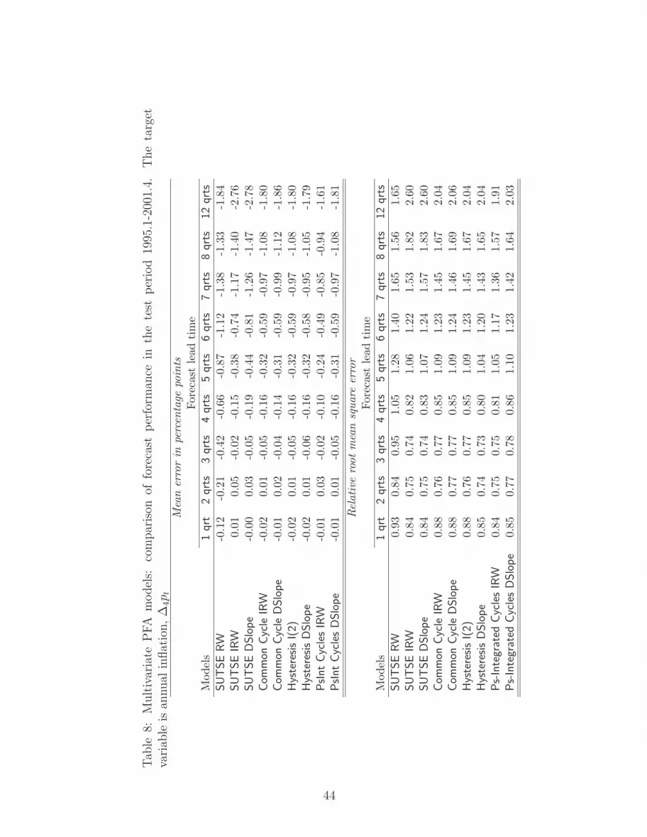
Tab

le8:

Mult

ivar

iate

PFA

model

s:co

mpar

ison

offo

reca

stper

form

ance

inth

ete

stper

iod

1995

.1-2

001.

4.T

he

targ

etva

riab

leis

annual

inflat

ion,∆

4p t

Mea

ner

ror

inpe

rcen

tage

poin

tsFo

reca

stle

adti

me

Mod

els

1qrt

2qrt

s3

qrt

s4

qrt

s5

qrt

s6

qrt

s7

qrt

s8

qrt

s12

qrt

s

SU

TSE

RW

-0.1

2-0

.21

-0.4

2-0

.66

-0.8

7-1

.12

-1.3

8-1

.33

-1.8

4SU

TSE

IRW

0.01

0.05

-0.0

2-0

.15

-0.3

8-0

.74

-1.1

7-1

.40

-2.7

6SU

TSE

DSlo

pe

-0.0

00.

03-0

.05

-0.1

9-0

.44

-0.8

1-1

.26

-1.4

7-2

.78

Com

mon

Cyc

leIR

W-0

.02

0.01

-0.0

5-0

.16

-0.3

2-0

.59

-0.9

7-1

.08

-1.8

0Com

mon

Cyc

leD

Slo

pe

-0.0

10.

02-0

.04

-0.1

4-0

.31

-0.5

9-0

.99

-1.1

2-1

.86

Hys

tere

sis

I(2)

-0.0

20.

01-0

.05

-0.1

6-0

.32

-0.5

9-0

.97

-1.0

8-1

.80

Hys

tere

sis

DSlo

pe

-0.0

20.

01-0

.06

-0.1

6-0

.32

-0.5

8-0

.95

-1.0

5-1

.79

PsInt

Cyc

les

IRW

-0.0

10.

03-0

.02

-0.1

0-0

.24

-0.4

9-0

.85

-0.9

4-1

.61

PsInt

Cyc

les

DSlo

pe

-0.0

10.

01-0

.05

-0.1

6-0

.31

-0.5

9-0

.97

-1.0

8-1

.81

Rel

ativ

ero

otm

ean

squa

reer

ror

Fore

cast

lead

tim

eM

odel

s1

qrt

2qrt

s3

qrt

s4

qrt

s5

qrt

s6

qrt

s7

qrt

s8

qrt

s12

qrt

s

SU

TSE

RW

0.93

0.84

0.95

1.05

1.28

1.40

1.65

1.56

1.65

SU

TSE

IRW

0.84

0.75

0.74

0.82

1.06

1.22

1.53

1.82

2.60

SU

TSE

DSlo

pe

0.84

0.75

0.74

0.83

1.07

1.24

1.57

1.83

2.60

Com

mon

Cyc

leIR

W0.

880.

760.

770.

851.

091.

231.

451.

672.

04Com

mon

Cyc

leD

Slo

pe

0.88

0.77

0.77

0.85

1.09

1.24

1.46

1.69

2.06

Hys

tere

sis

I(2)

0.88

0.76

0.77

0.85

1.09

1.23

1.45

1.67

2.04

Hys

tere

sis

DSlo

pe

0.85

0.74

0.73

0.80

1.04

1.20

1.43

1.65

2.04

Ps-

Inte

grat

edCyc

les

IRW

0.84

0.75

0.75

0.81

1.05

1.17

1.36

1.57

1.91

Ps-

Inte

grat

edCyc

les

DSlo

pe

0.85

0.77

0.78

0.86

1.10

1.23

1.42

1.64

2.03

44