Estimation of the refractive index structure parameter fromsingle-level daytime routine weather data
A. van de Boer,1, 2, ∗ A.F. Moene,1 A. Graf,3 C. Simmer,2 and A.A.M. Holtslag1
1Meteorology and Air Quality Section, Wageningen University, The Netherlands2Meteorological Institute University Bonn, Germany
3Agrosphere Institute, Forschungszentrum Julich, Germany
compiled: July 29, 2014
Atmospheric scintillations cause difficulties for applications where an undistorted propagation of elec-tromagnetic radiation is essential. These scintillations are related to turbulent fluctuations of temper-ature and humidity that are in turn related to surface heat fluxes. We developed an approach thatquantifies these scintillations by estimating Cn2 from surface fluxes that are derived from single-levelroutine weather data. In contrast to previous methods that are biased to dry and warm air, ourmethod is directly applicable to several land-surface types, environmental conditions, wavelengths,and measurement heights (look-up tables for a limited number of site-specific parameters are pro-vided). The approach allows for an efficient evaluation of the performance of e.g. infrared imagingsystems, laser geodetic systems, and ground-to-satellite optical communication systems. We testedour approach for two grass fields in central and southern Europe, and for a wheat field in centralEurope. Although there are uncertainties in the flux estimates, the impact on Cn2 is shown to berather small. The Cn2 daytime estimates agree well with values determined from eddy covariancemeasurements for the application to the three fields. However, some adjustments were needed for theapproach for the grass in southern Europe because of non-negligible boundary-layer processes thatoccur in addition to surface-layer processes.
OCIS codes: (010.1330) Atmospheric and oceanic optics, Atmospheric turbulence; (010.3920)Meteorology; (010.1300) Atmospheric propagation; (010.3310) Laser beam transmission; (010.7295)Visibility and imaging.
http://dx.doi.org/10.1364/XX.99.099999
1. IntroductionAtmospheric turbulence and the related fluctua-tions of the refractive index of air affect the prop-agation of electromagnetic waves. These so calledscintillations are a challenge for communication andimaging systems (e.g. ground-based telescopes)that use radio waves, visible, or infrared radia-tion [1]. Fluctuations in the refractive index of airare mainly related to temperature and humidity.Therefore, turbulent fluctuations of temperatureand humidity determine the intensity of turbulence-induced refraction. Various instruments and calcu-lation methods have been developed to obtain thestructure parameter of the refractive index of air(Cn2) for a certain wavelength, to qualify signals of
∗ Corresponding author: [email protected]
imaging or communication systems that use elec-tromagnetic radiation. However, these instruments(sonic anemometer, scintillometer, air refractome-ter) are not easy to operate and rather expensive,such that frequent observations are rare. A ro-bust method to quantitatively estimate Cn2 basedon readily available data is therefore needed. Ourmethod could moreover be used for gap-filling incase of failures of a sonic anemometer, scintillome-ter, or an air refractometer.
Already forty years ago, [2] developed a semi-empirical theory which relates the temperaturestructure parameter CT 2 (which is related to Cn2)to atmospheric stability and the vertical tempera-ture gradient at a certain height in the atmosphericsurface layer (the lowest meters of the atmosphere).In the years after, several studies showed that Cn2
does not only depend on CT 2 , but also on the hu-midity structure parameter Cq2 and on the joint

2
structure parameter CTq [3]. For wavelengths inthe visible and near-infrared, Cn2 mainly dependson CT 2 , while for radio wavelengths, Cq2 mainlydetermines Cn2 . A summary of past research onmodels and measurements for optical turbulence ispresented in [1]. [4] and [5] estimated Cn2 fromdual-level meteorological data over the ocean forvisible light. [6] performed a sensitivity study fora) a Cn2 derivation method based on observed sur-face fluxes of heat, moisture and momentum usingMonin-Obukhov similarity theory [7], and for b)a method based on dual-level meteorological data.He tested both methods above snow for a broadwavelength range (visible, infrared, millimeter, andradio).
However, fluxes or vertical gradients are usuallynot available from regular meteorological observa-tions. Therefore, [8] developed a regression-basedmethod based on single-level standard weather-station data to estimate Cn2 in the atmosphericsurface layer, restricted to one height and one wave-length. Also, weather forecasts can be used to pre-dict Cn2 by their method. The method needs, how-ever, several empirical parameters which were onlyderived for a desert region, and which need to befirst determined for other regions. [9] and [10] devel-oped methods to similarly obtain Cn2 from single-level weather data for prairie grasslands and coastalenvironments, which are, however, also not appli-cable for other regions. [11] evaluated three modelsthat are all based on work of [8] and [10]. They com-pared model output with scintillometer data of twodays atop a mountain in Florida, and found mod-erate results. Besides the regional limitation, thesemodels also only hold for optical wavelengths. [12]used Large Eddy Simulation on weather forecasts,to characterize near-surface optical turbulence atfour sites in western Europe. However, new, ro-bust, and easy-to-use methods for estimating Cn2
from single-level weather data are lacking, whichmotivates our study.
The daily course of Cn2 depends on the atmo-spheric conditions which depend on the time of theday, the day of the year (DOY), the weather type ofthat specific day, and the vegetation activity. Ob-servations of Cn2 above grass in the Netherlands aregiven in Fig. 1 for cloudy and clear sky conditions,for a summer and an autumn day, for an opticaland a millimeter wavelength. With our scheme, weaim to capture both the daily and seasonal changesof Cn2 for different locations.
We use an adaptation of the scheme introducedby [13] and [14], later referred to as dRH99, that
estimates surface heat and moisture fluxes fromair temperature, humidity, pressure, wind speedand incoming shortwave radiation all measured atone height only. This scheme is based on thePenman-Monteith equation, which estimates evap-otranspiration rates from atmospheric conditionsand vegetation specific parameters (e.g. canopy re-sistance, surface albedo and roughness) that are alleasy to estimate. We provide look-up tables forthese parameters in Section 2.A and in the Appen-dices, where we describe our implementation of thescheme. In Section 2, we furthermore explain howCT 2 , Cq2 and CTq are derived from surface fluxes(using Monin-Obukhov similarity theory), and howCn2 is derived from the meteorological structure pa-rameters. Our method is easily applicable, and canbe used to provide insight in optical turbulence at aspecific location for a certain moment, but also fora period of several years to derive its climatology.Estimates of optical turbulence effects on electro-optic or laser systems could be derived, mainly forhorizontal atmospheric paths, as a forecast, or dur-ing or after a specific operation. The completescheme that estimates Cn2 from standard single-level weather data follows from the Appendix andSection 2.B and 2.C.
We validate estimated fluxes and structure pa-rameters with summertime measurements from dif-ferent locations and vegetation types: grass in theNetherlands, grass in the South of France, andwheat in the West of Germany. Each dataset cov-ers at least one month of data. In Section 3, wedescribe the datasets, and in Section 4 we explainthe evaluation of our scheme. We restrict ourselvesto daytime data, because in our current implemen-tation, we miss information to estimate incominglong-wave radiation at night time. In Section 5, wecompare fluxes and structure parameters derivedusing our method with high frequency measure-ments (eddy covariance). In Section 6 we presentthe weaknesses of previous methods, and we showthe sensitivity of our own scheme. In contrast toother methods, our scheme only weakly depends onempirical assumptions and is still computationallycheap.
2. Framework
In this section, we describe how we derive Cn2 fromthe atmospheric variables temperature, humidity,pressure, wind speed and radiation, and from thesurface characteristics albedo, roughness, leaf areaindex, vegetation height and the minimal stomatalresistance of the canopy. Our scheme follows threesteps. First (Section 2.A), fluxes are estimated from

3
0 6 12 18 2410
−16
10−15
10−14
10−13
10−12
Time [h]
Cn2λ=
670nm
[m−2/3]
a 19 Jun clear5 Jul cloudy
0 6 12 18 2410
−14
10−13
10−12
10−11
10−10
Time [h]
Cn2λ=
2mm
[m−2/3]
b
0 6 12 18 2410
−16
10−15
10−14
10−13
10−12
Time [h]
Cn2λ=
670nm
[m−2/3]
c 14 Sep clear18 Sep cloudy
0 6 12 18 2410
−14
10−13
10−12
10−11
10−10
Time [h]
Cn2λ=
2mm
[m−2/3]
d
Fig. 1. Daily course of observed values of Cn2 for λ = 670nm (a and c) and λ = 2mm (b and d) for different weathertypes (blue asterisk is clear sky, red circle is cloudy) and seasons; two summer days (a and b) and two autumn days(c and d) above grass in the Netherlands (Haarweg Wageningen, 2005).
the single-level weather data using an adaptationof an existing scheme based on a linearized ver-sion of the surface energy balance and the Penman-Monteith equation. Then (Section 2.B), the ob-tained fluxes are used to estimate the structureparameters CT 2 , Cq2 and CTq2 , following Monin-Obukhov similarity theory. Cn2 is finally estimatedfrom the latter (Section 2.C) using theory describedby [15].
2.A. Estimation of surface fluxes from single-level weather data
2.A.1. Basic method
dRH99 presented a scheme that relates surfacefluxes of momentum and sensible and latent heatto only a few weather variables. They success-fully tested their scheme for a full year of obser-vations above grass in Cabauw, the Netherlands.The scheme is based on a linearized version of thesurface energy balance equation, where every de-pendence of a flux on the surface temperature isreplaced by a linearized dependence on the temper-ature difference between surface and atmosphere.
For the evapotranspiration flux (LvE) this leads
to the Penman-Monteith equation
LvE =s(Qn −G) +
ρcpra
(esat − ea)
s+ γ(1 + rcra
), (1)
where Qn is the net radiation, G the soil heat flux,and rc and ra are the canopy and aerodynamic re-sistances which together determine the partition-ing between sensible and latent heat flux. For thecanopy resistance, a few site-specific input parame-ters are needed, for which we here provide a lookuptable (Table 1 and Table 7). esat − ea is the watervapor deficit in Pa, where ea is the actual water va-por pressure and esat is the saturation water vaporpressure (which only varies with temperature). sis the slope of the saturated vapor pressure curve,ρ is the air density, cp is the specific heat capac-ity of air at constant pressure (p) that depends onhumidity, and γ is the psychrometric constant (allgiven in Appendix A). Note that Eq. 1 describestranspiration only. However, if rc would be set tozero, evaporation of intercepted water is simulated.
The sensible heat flux H can be calculated as aresidual of the surface energy balance
H = Qn −G− LvE. (2)

4
Table 1. Vegetation types and parameter values after theERA40 surface scheme (TESSEL) used in the ECMWFmodel.
Vegetation rs,min LAILow crops, mixed farming 180 3Irrigated low crops 180 3Short grass 110 2Tall grass 100 2Low shrubs 225 3Deciduous broad leaf trees 175 5Needle-leaf trees 500 5Tundra 80 1Desert 250 0.5
To obtain LvE, the estimation of the surface skintemperature is crucial because of its role in both Qn
and G. The estimation of the surface skin temper-ature depends on ra, however, H and LvE dependon ra as well. Therefore, the scheme consists of aniteration loop. ra depends on atmospheric stabil-ity, such that the surface skin temperature is esti-mated via an iteration that starts with a neutralatmosphere (further explained in Section 4). Thenet radiation and thus the available energy for heatfluxes further depends on the downward shortwaveradiation (Sin), the surface albedo (a), cloud cover,surface long-wave emissivity, and atmospheric long-wave emissivity.
2.A.2. Modifications to dRH99
Our scheme to solve Eq. 1 to estimate heat fluxesfrom single-level weather data is given in AppendixA, where is shown how all terms of the surface en-ergy balance are determined based on Sin, Ta, q, u(wind speed) and p. In this section, we discuss theadaptations that we made to the scheme of dRH99regarding rc and radiation calculations.
Because the scheme of dRH99 was only testedfor one specific location in the Netherlands (grass-covered), its performance for other regions or veg-etation types is uncertain. Here we focus on theparameterization of the dependence of the canopyresistance rc on water vapor content of the air.dRH99 use the following formulation:
rc = 104∆q = 104 esat − ea
p
Rd
Rv, (3)
where ∆q is the specific humidity deficit in kg kg−1,calculated as qsat − q, and Rd and Rv are the spe-cific gas constants for dry air and for water vaporrespectively; 287 and 462 J kg−1 K−1).
We here show a comparison of the approxima-
tions for the dependency of rc on water vapor deficitgiven by dRH99 and [16], referred to as BB97,and three approximations used in the land-surfaceschemes of the weather and climate models of a)the National Center for Meteorological Researchin France (CNRM, the ISBA-Ags scheme), b) theUnited States National Centers for Environmen-tal Prediction (NCEP, the Noah scheme), and c)the European Center for Medium-range WeatherForecasts (ECMWF, the TESSEL scheme). TheNoah and TESSEL schemes are based on the Jarvis-Stewart approach [17, 18], where
rc =rs,min
LAIfdqfradfT fθ. (4)
This approach is based on rs,min, a minimum stom-atal resistance for optimal conditions, which is veg-etation dependent (see Table 1), and that is scaledfrom a square meter of leaf surface to a canopy witha specific leaf area index (LAI, see Table 1 as well).The four functions represent the reaction of vege-tation to environmental factors: global radiation,water vapor deficit, air temperature, and soil mois-ture. In this discussion, we only address the watervapor deficit dependency. In Noah [19], fdq is cal-culated as 1 + hs ∆q [20], where hs is an empiricalcoefficient that describes the reaction of stomatalresistance on humidity deficit (≈45 kg kg−1, the in-verse of K3 in [21]). The Ags scheme [22] contains asimilar type of response, but with hs = 58 kg kg−1.
In TESSEL [23], fdq = egD85p∆q is used, which has
a similar effect as the Noah implementation (seeFig. 2) for gD = 0.02 mb−1 (in TESSEL, gD =0.03mb−1 for trees and zero for crops). BB97 calculate,based on Cabauw data, the canopy resistance as
rc = 25.9fdqfradfθ, (5)
where fdq = 1 + hs (∆q − ∆q0). hs =160 kg−1 kg,∆q0 = 0.003 kg−1 kg, and the factor 25.9 repre-sents a specific
rs,min
LAI . For comparison we need theapproach of BB97 in the Jarvis-Stewart format (Eq.4), leading to a scaling factor fr = 0.47, such that
frrs,min
LAI Cabauwfdq = 25.9 (1 + hs (∆q − ∆q0)) ,
(6)for LAI = 2 and rs,min = 110s m−1, being repre-sentative for Cabauw.
The approach of dRH99 significantly deviatesfrom the other approximations (Fig. 2). Their re-sponse function (and thus the canopy resistance)at zero water vapor deficit (relative humidity of100%) is zero. Herewith, dRH99 empirically take

5
0 5 10 15 20 250
1
2
3
4
5
∆ q [g kg−1]
f dq[-]
dRH99HTESSELNoahAgsBB97
Fig. 2. The reaction of rc to water vapor deficit ∆qaccording to different schemes for the observed range of∆q. The reactions by dRH99 and by BB97 were definedfor the same grass area (Cabauw, the Netherlands), andare therefore both calculated by rcLAI/rs,min (LAI = 2,rs,min = 110s m−1, being representative for Cabauw).
into account that at low water vapor deficits, theevapotranspiration term is dominated by evapora-tion whereas it is assumed in the Penman-Monteithequation that transpiration is the only contribu-tion to evapotranspiration. For the three land-surface schemes, the response function is one (rc =rs,min/LAI) for a saturated atmosphere (∆q = 0).The function of BB97 leads to a response value of0.24 for a saturated atmosphere (see Eq. 6).
The other difference is that the function of dRH99shows a much stronger increase of rc with ∆q thanthe other four functions, which leads to large devi-ations for dry air conditions (∆q > 10g kg−1). Thisis probably caused by the fact that they tested theirscheme only for a Dutch grassland (Cabauw), where∆q typically ranges between 5 and 11 g kg−1.
Given the above limitations, we replace the rep-resentation by dRH99 by a function that is also ap-plicable for other locations and land use types (e.g.a function with a small rc for very humid condi-tions and a weak dependence on ∆q). We howeverfound that in our data, rc calculated from the watervapor deficit dependency as in Noah, TESSEL andAgs, is very different from rc derived from measure-ments via the inverted Penman-Monteith equation.Namely, the values obtained with Noah, TESSEL,and Ags all stay within a very short range aroundrs,min/LAI. The function of BB97 is a nice integra-tion between a small offset and a weak slope of theresponse functions. In our scheme, we use Eq. 5,omitting fθ (see Appendix A), and we replace thescaling factor 25.9 by frrs,min/LAI.
To estimate incoming long-wave radiation,dRH99 use an expression given by [24], where Lin
depends on the apparent emissivity of the atmo-sphere, the fractions of low and high clouds, andtwo empirical cloud coefficients. However, as infor-mation on cloud cover for high and low clouds is notavailable in our datasets, we use relations describedin [25] for clear skies, and [26] for cloudy skies,which depend on the total cloud cover only (as de-tailed in Appendix A). We also slightly adapted thealbedo calculation of dRH99, such that it does notdepend on the fraction of diffuse radiation, but onthe total cloud cover fraction.
2.B. Estimation of structure parameters of tem-perature and humidity from surface fluxes
The relations between structure parameters andsurface fluxes, based on Monin-Obukhov similar-ity theory, have been studied by among others [2],[6], [27], [28], [29], and [30]. [31] found, from aLarge Eddy Simulation resolving surface layer tur-bulence, that the functions derived for CT 2 followMonin-Obukhov similarity theory, while the func-tions for Cq2 are sensitive and not universal. De-viations from Monin-Obukhov similarity theory formeasured variances were quantified as well, by [32].Here we use the universal functions for the structureparameters of temperature and humidity, for unsta-ble conditions presented by [30]. They describe therelation between the structure parameters and sur-face fluxes via the temperature and humidity scalesT∗ and q∗ (Eq. 15d in Appendix A) as
(κz)2/3CT 2
T 2∗
= 6.7κ2/3(1 − 14.9z
L)−2/3, (7a)
(κz)2/3Cq2
q2∗
= 3.5κ2/3(1 − 4.5z
L)−2/3. (7b)
In these equations, κ is the Von Karman constantwith a value of 0.4. z is the height of interest abovethe canopy, assuming that the atmospheric surfacelayer is a constant-flux layer: T∗ and q∗ do notchange with height. L is the Obukhov length de-fined by [33] as a function of surface friction andbuoyancy (see Appendix A).
For homogeneous turbulence, the joint structureparameter CTq can be estimated from the temper-ature and humidity structure parameters following[34]:
CTq = rTq
√CT 2Cq2 , (7c)

6
where rTq is the correlation coefficient between tem-perature and humidity. CTq has the value of thejoint structure function (scaled with a function ofthe separation distance) in the inertial subrange,assuming that rTq is similar for all scales withinthe inertial subrange. Usually, Ta and q fluctua-tions are better correlated in the inertial subrangethan at larger scales. For daytime data without dis-turbances from non-local processes, an rTq of 0.8 isoften observed close to the surface.
The step from surface fluxes to CT 2 and Cq2 in-troduces uncertainty in our Cn2-scheme, becauseMonin-Obukhov similarity theory is not alwaysvalid [32]. Also, the step from CT 2 and Cq2 to CTqintroduces uncertainty, because an estimate of rTqhas to be made (both issues are discussed in Section6).
2.C. Estimation of Cn2 from temperature, hu-midity and joint structure parametersThe relationship between the structure parameterof the refractive index of air n, and the temperature,humidity and joint structure parameter is given by[35] as
Cn2 =AT 2
Ta2 CT 2 +
Aq2
q2 Cq2 + 2ATAq
TaqCTq, (8a)
where AT and Aq depend mainly on pressure, airtemperature, specific humidity and the wavelength.Note that, although historically absolute humidityis used in the definitions of AT and Aq, here we willfollow [15] and use specific humidity. Functions forAT and Aq are given by [15] as
AT = − p
Ta
(b1 +
b2qRv
R
), (8b)
and
Aq = − p
Ta
bq2qRv
R
(1 − q (Rv −Rd)
R
), (8c)
where R is the universal gas constant (8.314 J K−1
mol−1). The wavelength dependency of AT andAq is captured by the coefficients b1 and bq2 (seeAppendix C).
3. DataIn the first part of this section we describe the threemeasurement sites, specifications on instrumenta-tion and vegetation, and the available data that weused to test our scheme. An overview of the mea-surements used for input or validation is given persite in Table 2. We test our scheme for two veg-
etation types (grass ’G’ and wheat ’W’), and twoclimatic regions (central ’C’ and southern Europe’S’). The names of the sites are: Haarweg (GC),Lannemezan (GS) and Merken (WC). In the secondpart of this section, we explain our data processingand selection.
3.A. Datasets
3.A.1. Haarweg: GC
The weather station at the Haarweg(http://www.met.wau.nl/haarwegdata) in Wa-geningen (the Netherlands, 7 m a.s.l.), anagro-meteorological station, provided all four ra-diation components and the soil heat flux (7.5 cmbelow ground level). In 2005, additionally, fluxesof sensible and latent heat were measured using aneddy-covariance (EC) station (3.2 m above groundlevel, a.g.l.). Over the year, the grassland wasmowed frequently to keep the vegetation height(zc) ≈ 10 cm. The soil at the Haarweg site containsclay and is rich in organic matter. We used datafrom the period 1 April to 30 September in 2005.
3.A.2. Merken: WC
Surface energy components were measured duringthe FLUXPAT campaign near Merken (Germany,114 m a.s.l.) in the summer of 2009. This cam-paign was organized to study the soil-vegetationatmosphere system (see e.g. [36] and [37] for de-tails). A station with an EC system (see Table 2for details) at 2.4 m a.g.l. was installed in the mid-dle of a flat winter wheat field. The four radiationcomponents were measured at 1.7 m a.g.l., and thesoil heat flux at 7.5 cm depth. The site containsa bouldered silt-loam soil. From 12 June on, thewheat height remained 0.85 m, which we specifiedas the start of the ripening process. Data from 15April to 12 June (DOY 104-163) were consideredas the growing phase of the wheat, and data from13 June to 26 July (DOY 164-207) as the ripen-ing phase. Canopy height and LAI measurementswere performed biweekly, such that we could derivea linear growth and LAI increase for the growingphase (see Table 3).
3.A.3. Lannemezan: GS
The BLLAST campaign (Boundary Layer Late Af-ternoon and Sunset Turbulence) took place near thePyrenees in southern France (582 m a.s.l.) from14 June to 8 July 2011 [38]. The main objec-tive of this campaign was to better understandthe physical processes that control and follow fromthe transition of a convective boundary layer to-wards a stratified nocturnal boundary layer. Sur-

7
face and boundary-layer measurements were per-formed around Lannemezan, a village located on alarge plateau (200 km2) with several mainly agri-cultural land use types on a sandy loamy soil. AnEC station was installed in a grass field, equippedwith sensors for the main surface energy compo-nents: sensible and latent heat flux (2.55 m a.g.l.),incoming and outgoing shortwave and long-wave ra-diation (1.68 m a.g.l.), and soil heat flux (3 cm be-low ground level), see Table 2 for details. The grasswas cut before the installation, and grew through-out the campaign reaching 35 cm at the end of thecampaign (see Table 3, we took zc = 0.25 m).
3.B. Data processing and selection
For the input of our scheme, we averaged 1-minutevalues of p and Sin to 30-minute data. Half-hourlywind speed, temperature and humidity values wereobtained from the eddy covariance data (as de-scribed below).
The long-wave radiation components and soilheat flux values were averaged for validation from 1-minute to 30-minute data as well. A storage termwas added to the soil heat flux using the calori-metric method [39], applying a volumetric soil heatcapacity of 2.2×10⁶ J m−3 K−1 for all three sites(assuming that the contributions of sand, clay, or-ganic matter, water and air are similar at the sites).
Eddy covariance data has been processed to pro-vide both mean variables (wind speed, temperatureand humidity) needed to drive the model, and fluxesand other turbulent quantities (see Table 2) thatwill be used to validate the model results. For thevalidation values, we determined averages of atmo-spheric stability, friction velocity and sensible andlatent heat fluxes from the 20 Hz EC-data (10 Hz inthe case of GC) using the software EC-pack-2.5.23-1.3 [40] for every measurement site. The averag-ing time was 30 minutes, which adequately cap-tures surface-layer turbulence and excludes meso-scale processes. For the heat fluxes, we performeda planar fit rotation [41] where the rotation angleswere determined over a period of 7 days to adjustthe coordinate system. Linear trends were removedand the Webb-correction [42] was applied to cor-rect humidity fluctuations for density fluctuationsinduced by temperature fluctuations. The sonictemperature (used as input) was corrected for hu-midity effects using the Schotanus correction [43].95% confidence intervals were estimated by quanti-fying the sampling error for each scalar average andflux, following [40], used for the data selection. Weused fixed upper and lower plausible limits for the
radiation and flux components. Because the sumof observed H and LvE is generally lower than theobserved available energy, we adjusted the sensibleand latent heat fluxes to the total available energy(Qn−G), while maintaining the value of the Bowenratio (H/LvE) following [44].
We also used the EC-pack software to obtain val-idation values for the structure parameters of Ta,q, and their joint structure parameter based on thestructure function. We applied path-averaging fac-tors to correct the structure parameters that arederived from measurements that originate from afinite path instead of one point. The correction forCT 2 related to a measurement height of 2.5 m, awind speed of 2 m s−1, the path length in the sonicanemometer of 0.12 m, and a lag of 0.9 m is a fac-tor of 1.12 following the Kaimal spectrum. For Cq2 ,this factor is 1.13 (with a path length in the gas an-alyzer of 0.13 m), and for CTq this factor is 1.49,which is higher because it additionally depends onthe distance between the anemometer and the gasanalyzer (0.15 m).
Furthermore, we applied a correction on thestructure parameters obtained by EC-pack (Eq.5 in [45]) to improve the conversion from timeto space (for a non-constant wind speed) that isneeded for the structure function following [46].They derived this correction factor for the struc-ture parameters from [47], who only determined it
forσ2UU2 < 0.1. If our data exceeded this limit, we ap-
plied a correction of 9590 (Eq. 5 in [45] for
σ2UU2 = 0.1).
To obtain Cn2 from the calculated structure param-eters, we used the expressions of [15] described inSection 2.C. We calculated Cn2 for an optical wave-length (λ = 670 nm) and for a millimeter wave-length (λ = 2 mm).
We selected daytime data between 7 and 17 UTCand eliminated stable situations by excluding datawith z/L > −0.02. Furthermore, we excluded datawhen less than 35980 raw data points were countedper half hour of 20 Hz data (17990 in the case ofGC). We also excluded rainy days from the data,because wet sonic anemometers and gas analyz-ers introduce errors in our liquidators Furthermore,turbulence in the lowest part of the atmosphere isvery weak on rainy days. For GC, we removed 36days such that 148 days remained. We also ex-cluded rainy days for WC, such that 44 days wereleft for the growing period, and 24 days for theripening period. For the grass data in SouthernFrance, we excluded 6 days (DOY 167, 169, 173,174, 180 and 185) at which rain events were ob-served (17 days remained).

8
Table 2. Instrumentation specifications per input or validation variable for the three measurement sites
Instrument Var. Usage Type and manufacturerInput Valid. Haarweg Merken & Lannemezan
Sonic anemometer Ta x CSAT3, Campbell Sci. CSAT3, Campbell Sci.u xu∗ xH xCT 2 x
Gas analyzer q x LI-7500, Li-cor LI-7500, Li-corLvE xCq2 x
Pyranometer Sin x CM11, Kipp & Zonen CNR1, Kipp & ZonenSout x
Pyrgeometer Lin x CG1, Kipp & Zonen CNR1, Kipp & ZonenLout x
Barometer p x PTB101B, Vaisala PTB101B, VaisalaSoil heat flux plate G x Thermopile, TNO HFP01SC, Hukseflux
4. Methods
Here we first describe how we use the scheme withour data, and then how we validate the scheme withother data and derivations.
From the 30-minute daytime data of Ta, q, p, uand Sin, we calculated the sensible, latent and soilheat fluxes, and the radiation components from thefirst step in our scheme as discussed in Section 2.A,following the parametrizations given in AppendixA. The required land-surface characteristics thatdiffer per measurement site are given in Table 3.Some constants are given in Appendix B.
From the estimated values for z/L, H, LvE, andu∗ that follow from the first part of the scheme, wecalculated the structure parameters CT 2 , Cq2 andCTq following the theory described in Section 2.B,applying a fixed rTq of 0.8. We derived Cn2 forλ = 670 nm and λ = 2 mm via Eq. 8.
We validated our estimates of the radiation com-ponents, fluxes and structure parameters with thevalues directly obtained by radiation and EC mea-surements. We also validate the key parametersand variables of the first part of our scheme: Ts, ra
and rc. These are however not directly measured.To compare the estimated surface temperature Ts
with measurements, we calculated the measured Ts
using
Ts =
(Lout − (1 − εs)Lin
εsσ
)1/4
(9)
in which we also used 0.96 for the surface emissivityεs, and 5.67×10⁻⁸ Wm−2K−4 for the Stefan Boltz-man constant σ. The measured resistances were
calculated following
ra = −ρcpTa − Ts
H, (10)
and
rc = ra
(s(Qn −G) +
ρcp(esat−ea)ra
γLvE− s
γ− 1
),
(11)which is an inverted form of the Penman-Monteithequation (Eq. 1).
We calculated regression fits per variable (var)for the four datasets, using orthogonal distance re-gression. The offset was set to zero, and the slopewas calculated, including its standard deviation.We normalized the RMSE by dividing by the meanobserved value of the specific variable to obtain theNRMSE to compare regressions of different vari-ables. Because the derivation of the measured re-sistances is sensitive for low fluxes and low availableenergy, we additionally eliminated data for the re-gression fit for rc and ra when H, LvE, or Qn−G <20 W m−2.
We tested the agreement of the datasets withMonin-Obukhov similarity theory by calculatingthe parameters in the similarity functions for thestructure parameters as follows: we kept the sec-ond parameter c2 in Eqs. 7a and 7b constant (14.9for T , 4.5 for q), and fitted the data to a regression
with the prescribed shape of y = c1 (1 − c2x)−2/3.The structure parameter and stability data wereweighted using the inverse of the confidence inter-vals for CT 2 , Cq2 , and z/L (via the intervals of u∗,

9
Table 3. Land-surface input variables per dataset. zc was measured, LAI was only measured at WC, the othervalues and the values for rs,min were taken from Table 1. LAT and LON are used for cloudiness calculations for thelong-wave radiation and albedo.
Variable GC WC grow WC ripe GSzc (m) 0.1 time dependenta 0.85 0.25LAI (m2 m−2) 2 time dependentb time dependentc 2rs,min (s m−1) 110 180 180 110LAT 51◦58’N 50◦50’N 50◦50’N 43◦07’NLON 5◦38’E 6◦24’E 6◦24’E 0◦21’E
a0.1 + 0.65DOY −10550
until DOY 163 (12 June), 0.85 m afterwardsb1.2 + 4.3DOY −105
35until DOY 140 (20 May), 5.5 afterwards
c5.5 − 5.5DOY −18321
after DOY 183 (2 July), 5.5 before
Ta, q, w′T ′ and w′q′) that were calculated by EC-pack
5. Results
We here discuss the results in the same steps and or-der as we described our scheme; first the estimationof fluxes from weather data (Section 5.A), then theestimation of temperature and humidity structureparameters from fluxes, and finally the estimationof Cn2 (Section 5.B).
5.A. Fluxes
The difference between the surface temperature Ts
and air temperature Ta is very important for thecalculation of the energy that is available for Hand LvE. This difference is however overestimatedfor all four datasets (see the regression fits and er-rors for all datasets in Table 4 and 5, and for GCFig. 3c). Despite the overestimation of this differ-ence, and thus of Ts, the long-wave radiation com-ponents are estimated fairly well for all datasets.Thereby, Qn estimates fit the observations with ageneral underestimation of 2-8% (see also Fig. 3ffor GC). For GS, this is caused by an underesti-mated incoming long-wave radiation. The surfacereflectance of shortwave radiation (albedo) is how-ever underestimated for all sites (not shown). G isunderestimated for all datasets. However, its valueis very low compared toQn such that this underesti-mation does not produce large errors for the energythat is available for H and LvE.rc estimates are much lower than the values we
derived from observations using the inverted Pen-man Monteith approach (Eq. 11) for all datasets.However, we did not validate our estimated rc withdirect observations, and thus the presented under-estimation of rc is uncertain. The NRMSE for rc
was despite the extra data selection still quite high.
Nevertheless, the partitioning of the available en-ergy into H and LvE is appropriate for GC andGS. This indicates that rc is of the correct orderof magnitude. For WC, H is generally overesti-mated, and LvE is slightly underestimated. How-ever, the estimations of all variables are quite scat-tered for the datasets (see the standard deviationsand NRMSE values given in the first columns in Ta-ble 5. The WC grow dataset is by far the smallestwe used, partly because of the stability criterion. ra
estimates are quite scattered, however, most of thedata used here is in a rc-regime in which the fluxesare not very sensitive to ra, see [48].
5.B. Structure parametersAlthough H and LvE are predicted well for GC,CT 2 and Cq2 and thereby CTq are overestimated.For the growing wheat (WC), H is largely overes-timated, which leads to a clear overestimation ofCT 2 as expected from the relation between H2 (orT 2∗ ) and CT 2 given in Eq. 7a. For GS, the regres-
sion slope for LvE is satisfying, whereas the slopefor Cq2 is more than twice as large. This is not ex-
pected from the relation between the slopes of LvE2
and Cq2 as mentioned above. We think that this ispartly related to the Monin-Obukhov parametersused for this relation. To check this hypothesis,we determined the similarity relationships (Eqs. 7aand 7b) where we kept c2 to its literature values of14.9 for temperature and 4.5 for humidity.
The obtained values for c1 deviate the most fromvalues given by [30] for the GS data, for both tem-perature and humidity (5.2 and 2.5 respectively,instead of 6.7 and 3.5). The coefficients for GCagree better with [30], with 6.7 and 3.9. For WC,we found 4.7 and 2.8 for the growing phase of thewheat (WC), and 4.7 and 2.6 for the ripening phase(WC). If we use the newly obtained coefficients for

10
Table 4. Regression results of estimated versus observed fluxes, structure parameters and variables at the Haarweg(GC left), based on 1071 half hourly averages (974 for rc and ra), and in Lannemezan (GS right), based on 220half hourly averages (177 for rc and ra). Indicated with ’MO’ are regression results using adapted Monin-Obukhovparameters for the scheme.
GC GSVar Slope NRMSE Slope NRMSEH 1.00 ± 0.01 0.05 0.86 ± 0.02 0.12LvE 1.01 ± 0.00 0.02 1.00 ± 0.01 0.02G 0.61 ± 0.01 0.81 0.69 ± 0.02 0.38Qn 0.98 ± 0.00 0.00 0.92 ± 0.00 0.01u∗ 0.90 ± 0.00 0.04 0.92 ± 0.01 0.05rc 0.73 ± 0.01 0.43 0.57 ± 0.02 0.80ra 1.28 ± 0.01 0.12 1.64 ± 0.05 0.25Ts − Ta 1.42 ± 0.01 0.14 1.38 ± 0.03 0.13Lin 0.98 ± 0.00 0.00 0.89 ± 0.00 0.02Lout 1.02 ± 0.00 0.00 1.01 ± 0.00 0.00CT 2 1.22 ± 0.01 0.12 1.48 ± 0.05 0.25Cq2 1.27 ± 0.02 0.17 2.32 ± 0.04 0.34CTq 1.26 ± 0.01 0.11 2.51 ± 0.07 0.40Cn2λ670nm 1.23 ± 0.01 0.13 1.35 ± 0.05 0.25Cn2λ2mm 1.28 ± 0.01 0.14 2.38 ± 0.04 0.35CT 2MO 1.12 ± 0.04 0.22Cq2MO 1.64 ± 0.03 0.19CTqMO 1.84 ± 0.05 0.27Cn2λ670nmMO 1.02 ± 0.04 0.25Cn2λ2mmMO 1.70 ± 0.03 0.19
Table 5. Regression results of estimated versus observed fluxes, structure parameters and variables during thegrowing season (left) in Merken (WC), based on 99 half hourly averages (83 for rc and ra), and during the ripeningseason (right), based on 283 half hourly averages (231 for rc and ra).
WC grow WC ripeVar Slope NRMSE Slope NRMSEH 1.20 ± 0.04 0.11 1.25 ± 0.02 0.09LvE 0.92 ± 0.02 0.04 0.94 ± 0.01 0.03G 0.56 ± 0.03 0.83 0.62 ± 0.02 0.55Qn 1.01 ± 0.01 0.02 0.97 ± 0.00 0.01u∗ 1.07 ± 0.01 0.02 1.24 ± 0.01 0.05rc 0.97 ± 0.09 0.66 0.69 ± 0.05 0.97ra 1.15 ± 0.06 0.20 1.10 ± 0.04 0.20Ts − Ta 1.65 ± 0.07 0.25 1.52 ± 0.04 0.20Lin 1.01 ± 0.00 0.00 1.01 ± 0.00 0.00Lout 1.01 ± 0.00 0.00 1.01 ± 0.00 0.00CT 2 2.02 ± 0.13 0.38 1.88 ± 0.06 0.29Cq2 1.18 ± 0.05 0.18 1.32 ± 0.03 0.15CTq 1.77 ± 0.10 0.33 1.73 ± 0.05 0.25Cn2λ670nm 2.04 ± 0.13 0.39 1.93 ± 0.06 0.30Cn2λ2mm 1.29 ± 0.06 0.20 1.40 ± 0.03 0.16

11
0 100 200 3000
100
200
300
r a mod
el [s
m−
1 ]ra obs [sm−1]
a
0 100 200
0
100
200
r c mod
el [s
m−
1 ]
rc obs [sm−1]
b
280 290 300 310 320280
290
300
310
320
Ts m
odel
[K]
Ts obs [K]
c
0 100 200 3000
100
200
300
H m
odel
[Wm
−2 ]
H obs [Wm−2]
d
0 200 400 6000
200
400
600
L vE m
odel
[Wm
−2 ]
LvE obs [Wm−2]
e
0 200 400 6000
200
400
600
Qn−G obs [Wm−2]
Qn−
G m
odel
[Wm
−2 ]
N
f
0
0.5
1
Fig. 3. Validation of estimates of ra, rc, Ts, H, LvE, and Qn − G with measurements at a grass field in theNetherlands (GC) in 2005. Dark markers indicate clear-sky conditions, whereas light markers indicate very cloudyconditions.
10−15
10−14
10−13
10−1210
−15
10−14
10−13
10−12
Cn2λ=670nm obs [m−2/3]
Cn2λ=670nmmodel
[m−2/3]
a
10−13
10−12
10−11
10−1010
−13
10−12
10−11
10−10
Cn2λ=2mm obs [m−2/3]
Cn2λ=2mm
model
[m−2/3]
b
N
0
0.5
1
Fig. 4. Validation of estimates of the structure param-eters of n for an optical (a) and a millimeter wave-length (b), with derivations from measurements at agrass field in the Netherlands in 2005. Dark markersindicate clear-sky conditions, whereas light markers in-dicate very cloudy conditions.
GS (5.2 and 2.5 for temperature and humidity re-spectively), we obtain improved regression slopes(indicated with MO in Table 4). However, Cq2is still overestimated (albeit with a large NRMSE)while the estimation of LvE is close to perfect witha very low NRMSE. The large NRMSE for Cq2 isprobably caused by the fact that at GS, humidityfluctuations were smaller than at GC and WC, andtherefore more sensitive to instrumental errors.
The estimates of CT 2 , Cq2 and CTq lead to rea-sonable estimates of Cn2 , see Tables 4 and 5 andFigs. 4 and 5. Note that the structure parametersoccur in a large range (mind the logarithmic scalein the figures, and hence a slope of 2 should be in-terpreted as an error of much less than an order
10−15
10−14
10−13
10−1210
−15
10−14
10−13
10−12
Cn2λ=670nm obs [m−2/3]
Cn2λ=670nmmodel
[m−2/3]
a
10−13
10−12
10−11
10−1010
−13
10−12
10−11
10−10
Cn2λ=2mm obs [m−2/3]
Cn2λ=2mm
model
[m−2/3]
b
N
0
0.5
1
10−15
10−14
10−13
10−1210
−15
10−14
10−13
10−12
Cn2λ=670nm obs [m−2/3]
Cn2λ=670nmmodel
[m−2/3]
a
10−13
10−12
10−11
10−1010
−13
10−12
10−11
10−10
Cn2λ=2mm obs [m−2/3]
Cn2λ=2mm
model
[m−2/3]
b
N
0
0.5
1
Fig. 5. Validation of estimates of the structure pa-rameters of n for an optical (a and c) and a millime-ter wavelength (b and d), with derivations from mea-surements. Above: a grass field in southern France in2011 for adjusted Monin-Obukhov parameters. Below:a wheat field in the ripening phase in western Germanyin 2009. Dark markers indicate clear-sky conditions,whereas light markers indicate very cloudy conditions.
of magnitude. For GS, we see the overestimationof Cq2 again in the estimate for Cn2 for λ = 2mmbecause at this wavelength, scintillations are moresensitive to humidity fluctuations than at nanome-ter wavelengths. For the growing season in Merken,

12
4 8 12 16 2010
−16
10−15
10−14
10−13
10−12
Time [h]
Cn2λ=
670nm
[m−2/3 ]
a19 Jun clear5 Jul cloudy19 Jun model5 Jul model
4 8 12 16 2010
−14
10−13
10−12
10−11
10−10
Time [h]
Cn2λ=
2mm
[m−2/3 ]
b
Fig. 6. Cn2 measured (markers) and estimated (lines)for a clear (circles) and cloudy (asterisks) summer day(19 June 12 UTC, 2005) at the Haarweg (similar to Fig.1).
we find the opposite. The large uncertainty of CT 2
for the data of both the growing and ripening phaseleads to an overestimation of Cn2 for λ = 670nm, awavelength at which Cn2 is more sensitive to tem-perature fluctuations.
As an example of the possible application of ourscheme, we show in Fig. 6 the performance of ourscheme for a sunny and cloudy day at the Haarweg(GC). The scheme estimates the turbulence at thecloudy day very well, and for the clear sky day thereis a slight overestimation. It can be seen that forthe optical wavelength, scintillation values are high-est around noon, decrease until sunset and increaseagain towards midnight. On the other hand, for themillimeter wavelength the scintillations decreases tozero in the night. Cloudy conditions weaken thescintillations. For these cases, our method performsbetter for λ = 2mm than for λ = 670nm, becausehumidity fluctuations are larger and better defined.
6. DiscussionWe here compare our method with previous meth-ods, and discuss the sensitivity of an existingmethod that is often used. Furthermore, comple-mentary to the validation of our method presentedabove, we show the sensitivity of our method.
6.A. Sensitivity of previous methodsExisting methods for determining Cn2 that arebased on single-level data only were developed for
daytime and night time data, for desert and moun-tain areas. Probably, that is because one impor-tant application that suffers from poor electromag-netic wave propagation is the ground-based tele-scope. We tested the algorithm that is often used,which is presented (Eq. 6) and compared with otherempirical algorithms in [11].
As mentioned in the introduction, other methodsfor the determination of Cn2 from single level me-teorological data are available in literature. Thesemethods are generally less complex in construction,being based on non-linear regressions to Ta, u, andrelative humidity (RH), and occasionally Sin. Themethods are ignorant of the properties of the un-derlying land, but tracing back their origin revealsthat they were derived for desert and mountain ar-eas, combining daytime and night time data. Wehave tried to assess the skill of these methods for ourdatasets but discovered a number of issues. First,the methods are only applicable to optical wave-lengths (exact wavelength unspecified) and for asingle height (not clearly specified, but turns outto be 15 meter). But above all, for a large partof our data, the methods give negative Cn2 values.Here we will more closely look at a method devel-oped by [10], based on work by [8]. This method ispresented in [49] as Eq. 15.4.34 (also tested in [11],Eq. 6). In Fig. 7, we show the sensitivity of thatmethod to RH and Ta (the sensitivity to u and Sin
is much weaker).
For a dry and warm atmosphere, the method re-sults in positive Cn2 values that are of the order ofmagnitude of our measurements. However, for hu-mid or colder areas, the method results in a nega-tive value, which is physically impossible. We usedthe method with RH and Ta taken from our GCdata :25th and 75th percentiles, represented by thediamond markers in Fig. 7. These values lead to avalue just around the zero line, indicated in the fig-ure. The 25th percentile of temperature combinedwith the 75th percentile of humidity lead to a neg-ative value (the upper left diamond). This showsthat the method does not work for other regionsthan desert-like areas.
Therefore, we recommend our method over pre-vious methods, especially when using optical or mi-crowave systems above other land-use types than adesert or mountain peak. Our method is howevernot yet suitable for night time data. It is beyond thescope of this paper, but for night time applications,we suggest to replace the cloud-fraction estimate(Eq. 13c) or the long-wave radiation estimates byparts of the semi-empirical nocturnal surface fluxes

13
0
0
0
T [K]
RH
[%]
280 290 300 310 32020
40
60
80
100
Cn2 [10−14m−2/3]
0
5
10
Fig. 7. Sensitivity of derivations of Cn2 using the algo-rithm given in [49], to RH and Ta. Diamond markersindicate the 25th and 75th percentile of RH and Ta forthe grass data of the Haarweg in 2005.
scheme by [50]. Furthermore, night-time data oftencorresponds stable conditions, for which the Monin-Obukhov equations described in Section 2.B shouldbe replaced by functions that are valid for a stableatmosphere. Once such a night-time scheme hasbeen implemented, it would be good to additionallytest the model for desert and mountain regions, andfor high elevations.
6.B. Sensitivity of our methodWe developed a method to estimate Cn2 fromsingle-level weather data that consists of threesteps:
a From single-level weather data to surfacefluxes
b From surface fluxes to structure parameters oftemperature and humidity
c From structure parameters to Cn2
For step a, we applied an existing scheme of dRH99that was developed for grass in the Netherlands(Cabauw). We adjusted their scheme for other fieldconditions, and tested it for another grass field inthe Netherlands, a grass field in southern France,and a wheat field in western Germany. This schemeis based on the Penman-Monteith equation, whichis an appropriate description of the process of tran-spiration. But this only holds provided that it isused with observations from the location of interest;a different surface results in different temperature,humidity and wind observations.
In our scheme, we replaced the water vapor deficitdependency of rc described by dRH99 as rc =104∆q by the approach of BB97. In Fig. 8 we showthe performance of the scheme for LvE and rc if weuse the water vapor deficit dependency described
0 100 200
0
100
200
rcmodel
[sm
−1]
rc obs [s m−1]
a
0 200 400 6000
200
400
600
LvE
model
[Wm
−2]
LvE obs [W m−2]
b
∆q [kg kg−1]
0
0.005
0.01
Fig. 8. rc and LvE for the Haarweg (GC) using theapproach for rc from dRH99, colored by ∆q (light is 0,dark is 10 g kg−1).
by dRH99. When comparing these results with theresults presented in Figs. 3b and 3e, we see that theestimation of the latent heat flux deteriorates whenusing the original dRH99 formulation, especially fordry conditions. This result agrees with Fig. 2, inwhich we see that the approach of dRH99 differsfrom the other approaches mainly for dry air con-ditions.
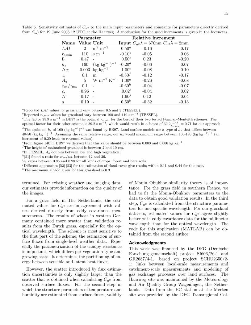
To investigate which parameters have the largestinfluence on the derived Cn2 , we performed a sensi-tivity analysis. In Table 6 we list the parameters ofstep a, and show for one midday summer situationthe relative increase of Cn2 for a realistic increaseof the parameters. We see that the dependency onthe parameters in fdq are very strong. Furthermore,our scheme is very sensitive to the estimated LAI,canopy height and albedo. This indicates that forthe first step of our method, a good estimate of thevegetation characteristics is the most crucial part.The increase of the parameters that lead to an in-crease or decrease of Cn2 for both wavelengths (e.g.N , a and Ag) are related to the available energy. Ifa certain increment leads to a decrease of Cn2 forone wavelength and an increase for the other wave-length, then the parameter is mainly related to thepartitioning of energy between latent and sensibleheat (e.g. LAI, rs,min and fr).
Next to the values given for the TESSEL land-surface scheme, we tested our method with vegeta-tion parameters from the Noah land-surface model(not shown). However, the flux and structure pa-rameter validation results are much worse using val-ues from Noah. It seems that the definition of LAIand rs,min cannot be separated from their appear-ance in the land-surface schemes. We did not imple-ment the dependency of rc on the type of carbonfixation the vegetation uses (C3 or C4). Addingsuch a plant-physiological process requires a clear

14
10−18
10−16
10−14
10−12
10−1010
−18
10−16
10−14
10−12
10−10
Cn
2 from obs CT
2, Cq
2 and CTq
[m−2/3]
Cn2
from
obs
T*, q
* and
rT
q [m−
2/3 ]
λ = 670nm y=0.94xλ = 2mm y=0.93x
Fig. 9. Validation of derivations of Cn2 from measuredvalues for CT 2 , Cq2 , CTq and rTq, with derivations fromflux measurements (T∗ and q∗) at a grass field in theNetherlands in 2005. Dark markers indicate an opticalwavelength, light markers indicate a millimeter wave-length.
separation between transpiration and evaporationprocesses. If Cn2 estimates are needed for partlywet vegetated surfaces, our method is empiricallysolid. However, we actually need a more realistictreatment to capture interception and soil evapora-tion. For that, a SVAT (soil vegetation atmosphere)could be used.
In step b, the uncertainties in the scheme are thevalidity of Monin-Obukhov similarity theory, andthe value for rTq. Furthermore, the derivations ofstructure parameters using EC-pack might intro-duce validation errors. Therefore, we also testedour scheme while by-passing step a: we determinedstructure parameters from observed fluxes (scaledas T∗ and q∗) rather than modeled fluxes. In Fig.9 we show that if measured fluxes are used, an al-most 1:1 fit is visible (for both wavelengths), withsome scatter for the lowest values. This means thateven if the flux estimation in the first step wouldbe perfect, Cn2 results will still be scattered.
Values for Cn2 calculated from measured fluxesusing Monin-Obukhov similarity theory are some-what smaller than Cn2 values derived from the ob-served structure parameters of Ta and q (see theslopes of the regression in the legend). This holdsfor both wavelengths for this data (GC), whichindicates that here, the Monin-Obukhov similar-ity functions for both temperature and humidityshould have a slightly larger c1 or smaller c2 (seeEqs. 7a and 7b). In the previous section we wrotethat, indeed, we found a slightly larger value for c1
for q for the GC data.
We found that for the GS dataset, we shouldcertainly change the coefficients in the Monin-Obukhov relations. In the previous section, we cal-culated c1 that fitted the data with a c2 that waskept constant. However, we would like to point outthat if we fit the GS data to the function withoutkeeping c2, we obtain for temperature c1 = 4.2 andc2 = 10.8, and for humidity c1 = 2.5 and c2 = 4.7.These values are very unusual compared to reportedvalues for several datasets [54], especially for hu-midity. However, more data in the neutral rangewould be needed for a good fit of c2.
Considering a fixed value for rTq, we cannot omitthis assumption when only weather data is avail-able, because rTq cannot be derived from low fre-quency temperature and humidity data. One wouldexpect a value close to one because temperatureand humidity are assumed to behave similar duringdaytime. We found in our datasets that the day-time values differ, with a median of ≈ 0.6 taking allscales together, which indicates that our datasetssuffered from non-local effects. However, this doesnot necessarily affect the correlation in the inertialsubrange. Therefore, the introduced error in thecalculation of CTq and therefore also in Cn2 by us-ing a fixed rTq of 0.8 is unknown.
Step c is the most straightforward part of ourmethod, because that part is based on establishedphysics theories. Only the dependency on the wave-length of interest influences the performance ofour method. For the tested datasets, our methodgenerally performs better for λ = 2mm than forλ = 670nm, due to a better defined humidity flux(microwaves are more sensitive to humidity fluctua-tions than to temperature fluctuations). Note thata more elaborated Cn2 scheme would also includethe scattering effect of aerosols on the wave propa-gation equation and thus on Cn2 .
7. Conclusions
A good estimation of the optical turbulence pro-vides knowledge on the performance of communi-cation and imaging systems. Often, weather datais available at only one level, precluding the use ofmethods based on vertical gradients [55]. There-fore, we here present an approach to estimate thestructure parameter of the refractive index of air(Cn2), based on single-level weather station data.Our estimates of Cn2 are accurate enough to help inthe development of systems based on the propaga-tion of electromagnetic waves (e.g. radio wave com-munication and ground-based telescopy). Based onlong time series of weather station data, the clima-tology of Cn2 for arbitrary wavelengths could be de-
15
Table 6. Sensitivity estimates of Cn2 to the main input parameters and constants (or parameters directly derivedfrom Sin) for 19 June 2005 12 UTC at the Haarweg. A motivation for the used increments is given in the footnotes.
Parameter Relative incrementName Value Unit Input Cn2λ = 670nm Cn2λ = 2mmLAI 2 m2 m−2 0.50a -0.16 0.17rs,min 110 s m−1 -0.10b -0.05 0.06fr 0.47 - 0.50c 0.23 -0.20hs 160 (kg kg−1)−1 -0.20d -0.06 0.07∆q0 0.003 kg kg−1 1.00e -0.08 0.10zc 0.1 m -0.80f -0.12 -0.17Ag 5 W m−2 K−1 1.00g -0.26 -0.08z0h/z0m 0.1 - -0.60h -0.04 -0.07εs 0.96 - 0.02i -0.04 0.02N 0.17 - 1.60j 0.12 0.04a 0.19 - 0.60k -0.32 -0.13
aReported LAI values for grassland vary between 0.5 and 3 (TESSEL).bReported rs,min values for grassland vary between 100 and 110 s m−1 (TESSEL).cThe factor 25.9 s m−1 in BB97 is the optimal rs,min for the best of their two tested Penman-Monteith schemes. Theoptimal factor for their other scheme is 39.2 s m−1, which would result in a factor of 39.2 LAI
rs,min= 0.71 for our approach.
dThe optimum hs of 160 (kg kg−1)−1 was found by BB97. Land-surface models use a type of hs that differs between40-50 (kg kg−1)−1. Assuming the same relative range, our hs would maximum range between 130-190 (kg kg−1)−1 (anincrement of 0.20 leads to reversed values).eFrom figure 14b in BB97 we derived that this value should be between 0.003 and 0.006 kg kg−1.fThe height of maintained grassland is between 2 and 10 cm.gIn TESSEL, Ag doubles between low and high vegetation.h[51] found a ratio for z0m/z0h between 12 and 26.iεs varies between 0.95 and 0.98 for all kinds of crops, forest and bare soils.jDifferent approaches [52] [53] for the estimation of cloud cover give results within 0.11 and 0.44 for this case.kThe maximum albedo given for this grassland is 0.3.
termined. For existing weather and imaging data,our estimates provide information on the quality ofthe images.
For a grass field in The Netherlands, the esti-mated values for Cn2 are in agreement with val-ues derived directly from eddy covariance mea-surements. The results of wheat in western Ger-many contained more scatter than validation re-sults from the Dutch grass, especially for the op-tical wavelength. The scheme is most sensitive tothe first part of the scheme; the estimation of sur-face fluxes from single-level weather data. Espe-cially the parametrization of the canopy resistanceis important, which differs per vegetation type andgrowing state. It determines the partitioning of en-ergy between sensible and latent heat fluxes.
However, the scatter introduced by flux estima-tion uncertainties is only slightly larger than thescatter that is obtained when calculating Cn2 fromobserved surface fluxes. For the second step inwhich the structure parameters of temperature andhumidity are estimated from surface fluxes, validity
of Monin Obukhov similarity theory is of impor-tance. For the grass field in southern France, wehad to fit the Monin-Obukhov parameters to thedata to obtain good validation results. In the thirdstep, Cn2 is calculated from the structure parame-ters for one specific wavelength. For our grasslanddatasets, estimated values for Cn2 agree slightlybetter with eddy covariance data for the millimeterwavelength than for the optical wavelength. Thecode for this application (MATLAB) can be ob-tained from the second author.
Acknowledgments
This work was financed by the DFG (DeutscheForschungsgemeinschaft) project SI606/26-1 andGR2687/4-1, based on project SCHU2350/2-1; links between local-scale measurements andcatchment-scale measurements and modeling ofgas exchange processes over land surfaces. TheHaarweg site was maintained by the Meteorologyand Air Quality Group Wageningen, the Nether-lands. Data from the EC station at the Merkensite was provided by the DFG Transregional Col-

16
laborative Research Center 32, TR32, Germany.The BLLAST field experiment was hosted by theinstrumented site of Centre de Recherches At-mospheriques, Lannemezan, France (ObservatoireMidi-Pyrenees, Laboratoire dAerologie). We thankthe anonymous reviewers for their positive feed-back.
Appendix A; Scheme to estimate fluxes fromweather data
The scheme to compute the surface fluxes consistsof four blocks. In the first block all variables thatcan be determined directly from the meteorologicalinput data are computed (Eqs. 12a-13g). The sec-ond block defines the dependence of the surface en-ergy balance on the surface temperature (Eqs. 14a-14i). The third block describes the iteration that isneeded to deal with the stability dependence (andhence surface-flux dependence) of the aerodynamicresistance (Eqs. 15a-15e). The final block describeshow, after convergence of the iteration, the variousenergy fluxes can be determined (Eqs. 16e-16a).
First, our scheme that is adapted from dRH99 di-rectly estimates air density ρ, air heat capacity cp(= 1004 (1 + 0.84q)), water vapor pressure ea andsaturated water vapor pressure esat (both in Pa)from air temperature (Ta), specific humidity (q) andpressure (p). The slope of the saturated vapor pres-sure curve is s(T ) = desat/dT , and the psychromet-ric constant is γ = cppRv/(LvRd), where Rd is thespecific gas constant for dry air (287 Jkg−1K−1),and Rv is the specific gas constant for water vapor(462 Jkg−1K−1). The temperature dependency ofesat, s and Lv can be found in [56], page 355.
After that, the surface resistance can be calcu-lated following
rc = frrs,min
LAIfdqfrad (12a)
where the scaling factor fr = 0.47, and fdq is calcu-lated following BB97:
fdq = 1 + hs (∆q − ∆q0) , (12b)
in which ∆q is the specific humidity deficit inkg kg−1 (calculated as qsat − q), hs =160 kg−1 kg,∆q0 = 0.003 kg−1 kg), and where
frad =1000Sin + 230 (1000 − 2Sin)
Sin (1000 − 230). (12c)
Then, most of the radiation components can becalculated. Outgoing shortwave radiation (Sout) is
calculated following
Sout = aSin, (13a)
where a is the surface albedo that depends on thesolar elevation angle α and the effective cloud coverfraction N as
a = amax − (1 −N) sin (α) (amax − amin)
−N (amax − acloud) .(13b)
amax, amin, and acloud are the surface albedo’s forrespectively a minimum solar elevation and a clearsky (the highest a), a maximum solar elevation anda clear sky (the lowest a), and a very cloudy sky(see Table 7 for the constants). We calculated N as
N =
Sin,0−Sin
Sin,0− 0.2
0.8, (13c)
where Sin,0 is the solar constant I0 (≈ 1365 W2m−2)multiplied with the cosine of the zenith angle θz ofthe specific location and time and corrected for theorbital eccentricity via the difference in distance (d)to the sun,
Sin,0 = I0
(dsun
dsun
)2
cosθz. (13d)
Incoming long-wave (L) radiation is calculated as
Lin = εaσT4a , (13e)
where εa is the air emissivity, and σ is the StefanBoltzmann constant (5.67 ×10⁻⁸). We used the fol-lowing expressions for the emissivity of air, adaptedfrom [25]
εa,clear = 0.63 + 5.95 × 10⁻⁷eae1500/Ta , (13f)
and [26]
εa = N + (1 −N) εa,clear. (13g)
Secondly, H is calculated from the energy balanceequation, which we can write as
H = Qn,0 +Qn,T (Ts − Ta) −G0 −GT (Ts − Ta)
−LvE0 − LvET (Ts − Ta),(14a)
where all energy terms consist of an isothermal termthat is calculated using Ta instead of Ts (indicatedwith the subscript 0), and a correction term thatcorrects for that assumption of an isothermal atmo-

17
sphere. This correction term therefore depends on(Ts−Ta) (indicated with the subscript T ). Thereby,the correction terms depend on H, via
Ts − Ta =Hra
ρcp. (14b)
Because ra depends on the atmospheric stabilitywhich is unknown, an iteration loop is needed tocalculate H. Inserting the H-dependent correctionterms in Eq. 14a results in
H =Qn,0 −G0 − LvE0
1 +Qn,T +GT + LvET, (14c)
where the isothermal terms are calculated following
Qn,0 = (1 − a)Sin + (εa − 1)εeσT4a , (14d)
G0 = Ag (Ta − T24h) . (14e)
Here, Ag is the soil heat transfer coefficient (seeTable 7), and T24h is the temperature history of thelast 24 h that represents the deep-soil temperature,and
LvE0 =ρcpγ
esat − e
ra + rc. (14f)
Note that LvE0 depends on ra too, which meansthat the calculation of LvE0 is part of the iterationloop that is used for the calculation of H.
The correction terms are all part of the itera-tion loop, because via H, we introduced an ra-dependency. The iteration loop for the energy bal-ance components (Eqs. 14c − 15e) is initiated withneutral conditions, and is stopped when the sensi-ble heat flux converged within 1 Wm−2 (3 iterationsare usually enough):
Qn,T =ra
ρcpεsσ4T 3
a , (14g)
where εs is the surface emissivity (see Table 7),
GT =ra
ρcpAg, (14h)
and
LvET =ra
γ
s (Ta)
ra + rc. (14i)
The loop starts with neutral conditions (ΨT =Ψu = 0) for a first estimate of the atmospheric-stability dependent ra and u∗. The aerodynamic
resistance is calculated as
ra =1
κu∗
(ln
z
z0h− ΨT
( zL
)+ ΨT
(z0h
L
)).
(15a)κ is the Von Karman constant (0.4), z the height(z = zm − d, d = 2
3zc is the displacement height),z0h is the roughness length for heat, calculated as0.1z0m (z0m = 0.4 (zc − d), the roughness length formomentum). ΨT is the Businger-Dyer integratedMonin-Obukhov flux profile relation function fortemperature gradients as described in [57]. L isthe Obukhov length calculated following Eq. 15c,and the friction velocity u∗ is calculated as
u∗ =uκ
ln(
zz0m
)− Ψu
(zL
)+ Ψu
(z0mL
) , (15b)
where u is the wind speed, Ψu is the Businger-Dyer integrated Monin-Obukhov flux profile re-lation function for wind speed gradients. TheObukhov length L is calculated within the loop as
L =Tau
2∗
κgTv∗, (15c)
where the temperature scale Tv∗ is a scaled buoy-ancy flux. The scalar scales are calculated as
Tv∗ =−Hv
ρcpu∗, T∗ =
−Hρcpu∗
, q∗ =−LvE
Lvρu∗(15d)
where the buoyancy flux
Hv = H (1 + 0.61q) + 0.61cpTaLvE0
Lv(15e)
and g is the acceleration due to gravity (9.81m s−2).
After H converged to one value, the followingvariables are extracted explicitly for diagnosis:
Ts = Ta +Hra
ρcp+ zΓd, (16a)
where Γd is the dry adiabatic lapse rate of 0.01Km−1. If Ts is known, the long-wave outgoing ra-diation, net radiation, and soil and latent heat fluxcan be calculated following
Lout = εsσT4s + (1 − εs)Lin, (16b)
Qn = Sin−Sout+Lin−Lout = Q0−εsσ4T 3a (Ts − Ta) .
(16c)

18
G = −Ag (T24h − Ts) = G0 +Ag (Ts − Ta) , (16d)
and
LvE =s (Qn −G) +
ρcpra
(esat − ea)
s+ γ(
1 + rcra
)= LvE0 +
ρcpγ
s (Ta) (Ts − Ta)
ra + rc.
(16e)
Appendix B; Land-surface input
Table 7. Land-surface input variables used for all sites(kept constant in our study although they can be sitedependent). The albedo’s amax, amin, and acloud areused for shortwave radiation calculations in Eq. 13b, andεs is the surface emissivity used for long-wave radiationcalculations. Ag determines the heat transfer betweenthe vegetation top and the soil in W m−2 K−1.
Parameter Valueamax 0.3amin 0.17acloud 0.21εs 0.96Ag 5rTq 0.8
Appendix C; Coefficients capturing the wave-length dependency of Cn2
For λ < 1 mm
b1 = 10−6
(0.237134 + 68.39397
130 − λ−2+
0.45473
38.9 − λ−2
),
(17a)
b2 = 10−6(0.648731 + 5.8058 × 10⁻³λ−2
−7.115 × 10⁻⁵λ−4 + 8.851 × 10⁻⁶λ−6 − b1,(17b)
bq2 = b2, (17c)
and for λ > 1 mm
b1 = 0.776 × 10⁻⁶, (17d)
b2 = 10−6
(7500
Ta− 0.056
), (17e)
bq2 = 10−6
(3750
Ta− 0.056
). (17f)
References
[1] A. Tunick, “A critical assessment of selected past re-search on optical turbulence information in diversemicroclimates,” Tech rep, Army Research Labora-tory (2002).
[2] J. C. Wyngaard, O. R. Cote, and Y. Izumi, “Localfree convection, similarity, and the budgets of shearstress and heat flux,” J Atmos Sci 28, 1171–1182(1971).
[3] M. L. Wesely, “The Combined Effect of Tempera-ture and Humidity Fluctuations on Refractive In-dex,” J Appl Meteor 15, 43–49 (1976).
[4] C. A. Friehe, “Estimation of the refractive-indextemperature structure parameter over the ocean.”Appl Opt 16, 334–340 (1977).
[5] K. L. Davidson, T. M. Houlihan, C. W. Fairall,and G. E. Schacher, “Observation of the temper-ature structure function parameter, C T 2, over theocean,” Bound-Layer Meteor 15, 507–523 (1978).
[6] E. L. Andreas, “Estimating Cn2 over snow and seaice from meteorological data,” JOSA A 5, 481–495(1988).
[7] A. S. Monin and A. M. Obukhov, “Basic laws ofturbulent mixing in the surface layer of the atmo-sphere,” Tr Geofiz Inst, Akad Nauk SSSR 24, 163–187 (1954).
[8] D. Sadot and N. S. Kopeika, “Forecasting opticalturbulence strength on the basis of macroscale mete-orology and aerosols : models and validation,” OptEng 31, 200–212 (1992).
[9] H. Rachele and A. Tunick, “Energy balance modelfor imagery and electromagnetic propagation,” JAppl Meteor 33, 964–976 (1994).
[10] S. Bendersky, N. S. Kopeika, and N. Blaunstein,“Atmospheric optical turbulence over land in mid-dle east coastal environments: prediction model-ing and measurements.” Appl Opt 43, 4070–4079(2004).
[11] T. T. Leclerc, R. L. Phillips, L. C. Andrews, D. T.Wayne, P. Sauer, and R. Crabbs, “Prediction ofthe ground-level refractive index structure param-eter from the measurement of atmospheric condi-tions,” Proc SPIE 7685, 76850A-76850A-8 (2010).
[12] S. Cheinet, A. Beljaars, K. Weiss-Wrana andY. Hurthaud, “The Use of Weather Forecaststo Characterise Near-Surface Optical Turbulence,”Bound-Layer Meteor 138, 453–473 (2011).
[13] A. A. M. Holtslag and A. P. Van Ulden, “A SimpleScheme for Daytime Estimates of the Surface Fluxesfrom Routine Weather Data,” J Climate Appl Me-teor 22, 517–529 (1983).
[14] W. C. de Rooy and A. A. M. Holtslag, “Estimationof surface radiation and energy flux densities fromsingle-level weather data,” J Appl Meteor 38, 526–540 (1999).

19
[15] H. C. Ward, J. G. Evans, O. K. Hartogensis, A. F.Moene, H. A. R. De Bruin, and C. S. B. Grim-mond, “A critical revision of the estimation of thelatent heat flux from two-wavelength scintillome-try,” Quart J Roy Meteor Soc (2013).
[16] A. Beljaars, and F. C. Bosveld, “Cabauw Data forthe Validation of Land Surface ParameterizationSchemes,” J Climate 10, 11721193 (1997).
[17] P. G. Jarvis, “The interpretation of the variationsin leaf water potential and stomatal conductancefound in canopies in the field,” Phil Trans 273, 593–610 (1976).
[18] J. B. Stewart, “Modelling surface conductance ofpine forest,” Agric Forest Meteor 43, 19–35 (1988).
[19] F. Chen, K. Mitchell, J. Schaake, Y. Xue, H. L. Pan,V. Koren, Q. Y. Duan, M. Ek, and A. Betts, “Mod-eling of land surface evaporation by four schemesand comparison with FIFE observations,” J Geo-phys Res 101 D3, 7251–7268 (1996).
[20] F. Chen and J. Dudhia, “Coupling an advancedland surface-hydrology model with the Penn State-NCAR MM5 modeling system. Part I: Model im-plementation and sensitivity,” Mon Wea Rev 129,569–585 (2001).
[21] J. Stewart and L. Gay, “Preliminary modelling oftranspiration from the fife site in Kansas,” AgricForest Meteor 48, 305–315 (1989).
[22] R. J. Ronda, H. A. R. de Bruin, A. A. M. Holtslag,“Representation of the canopy conductance in mod-eling the surface energy budget for low vegetation,”J. Appl. Meteor. 40, 1431-1444 (2001).
[23] B.J.J.M. van den Hurk, P. Viterbo, A.C.M. Bel-jaars, and A.K. Betts, “Offline validation of theERA40 surface scheme,” Technical report ECMWF,43p (2000).
[24] G. W. Paltridge and C. M. R. Platt, Radiative pro-cesses in meteorology and climatology (Amsterdam-Oxford-New York, Elsevier Scientific PublishingCompany, 1976).
[25] S. B. Idso, “A set of equations for full spectrum and8 to 14 µm and 10.5 to 12.5 µm thermal radiationfrom cloudless skies,” Water Resour Res 17, 295–304 (1981).
[26] T. M. Crawford and C. E. Duchon, “An ImprovedParameterization for Estimating Effective Atmo-spheric Emissivity for Use in Calculating DaytimeDownwelling Longwave Radiation,” J Appl Meteor38, 474–480 (1999).
[27] R. J. Hill, “Review of optical scintillation methodsof measuring the refractive-index spectrum, innerscale and surface fluxes,” Wave Random Media 2,179–201 (1992).
[28] V. Thiermann and H. Grassl, “The measurementof turbulent surface-layer fluxes by use of bichro-matic scintillation,” Bound-Layer Meteor 58, 367–389 (1992).
[29] H. A. R. De Bruin, W. Kohsiek, and J. J. M. van denHurk, “A verification of some methods to deter-mine the fluxes of momentum, sensible heat, andwater vapour using standard deviation and struc-ture parameter of scalar meteorological quantities,”Bound-Layer Meteor 63, 231–257 (1993).
[30] D. Li, E. Bou-Zeid, and H. A. R. De Bruin, “Monin–Obukhov similarity functions for the structure pa-rameters of temperature and humidity,” Bound-Layer Meteor 145, 45–67 (2012).
[31] B. Maronga, “Monin-Obukhov similarity functionsfor the structure parameters of temperature and hu-midity in the unstable surface layer: results fromhigh-resolution large-eddy simulations,” J AtmosSci (2013).
[32] A. van de Boer, A. F. Moene, A. Graf,D. Schuttemeyer, and C. Simmer, “Detection of en-trainment influences on surface-layer measurementsand extension of Monin-Obukhov similarity the-ory,” Bound-Layer Meteor (2014).
[33] A. M. Obukhov, “Turbulence in an Atmospherewith a Non-uniform Temperature,” Tr Geofiz Inst,Akad Nauk SSSR 1, 95–115 (1946).
[34] A. F. Moene, “Effects of water vapour on the struc-ture parameter of the refractive index for near-infrared radiation,” Bound-Layer Meteor 107, 635–653 (2003).
[35] R. J. Hill and S. F. Clifford, “Modified spectrum ofatmospheric temperature fluctuations and its appli-cation to optical propagation,” JOSA 68, 892–899(1978).
[36] A. Graf, D. Schuttemeyer, H. Geiß, A. Knaps,M. Mollmann-Coers, J. H. Schween, S. Kol-let, B. Neininger, M. Herbst, and H. Vereecken,“Boundedness of Turbulent Temperature Probabil-ity Distributions, and their Relation to the VerticalProfile in the Convective Boundary Layer,” Bound-Layer Meteor 134, 459–486 (2010).
[37] A. van de Boer, A. F. Moene, and D. Schuettemeyer,“Sensitivity and uncertainty of analytical footprintmodels according to a combined natural tracer andensemble approach,” Agric Forest Meteor 169, 1–11(2013).
[38] M. Lothon, F. Lohou, D. Pino, F. Couvreux,E. R. Pardyjak, J. Reuder, J. Vila-Guerau deArellano, P. Durand, O. Hartogensis, D. Legain,P. Augustin, B. Gioli, I. Faloona, C. Yague,D. C. Alexander, W. M. Angevine, E. Bargain,J. Barrie, E. Bazile, Y. Bezombes, E. Blay-Carreras, A. van de Boer, J. L. Boichard, A. Bour-don, A. Butet, B. Campistron, O. de Coster,J. Cuxart, A. Dabas, C. Darbieu, K. Deboudt,H. Delbarre, S. Derrien, P. Flament, M. Four-mentin, A. Garai, F. Gibert, A. Graf, J. Groebner,F. Guichard, M. A. Jimenez Cortes, M. Jonassen,A. van den Kroonenberg, D. H. Lenschow, V. Magli-

20
ulo, S. Martin, D. Martinez, L. Mastrorillo, A. F.Moene, F. Molinos, E. Moulin, H. P. Pietersen,B. Piguet, E. Pique, C. Roman-Cascon, C. Rufin-Soler, F. Saıd, M. Sastre-Marugan, Y. Seity, G. J.Steeneveld, P. Toscano, O. Traulle, D. Tzanos,S. Wacker, N. Wildmann, and A. Zaldei, “Thebllast field experiment: Boundary-layer late after-noon and sunset turbulence,” Atmos Chem PhysDiscuss 14, 10789–10852 (2014).
[39] W. R. Rouse, “Microclimate at Arctic Tree Line 3.The Effects of Regional Advection on the SurfaceEnergy Balance of Upland Tundra,” Water ResourRes 20, 74–78 (1984).
[40] A. van Dijk, A. F. Moene, and H. A. R. de Bruin,“The principles of surface flux physics : theory ,practice and description of the ECPACK library,”Internal Report 2004/1, Meteorology and Air Qual-ity Group, Wageningen University, Wageningen, theNetherlands p. 99 pp. (2004).
[41] J. M. Wilczak, S. P. Oncley, and S. A. Stage, “Sonicanemometer tilt correction algorithms,” Bound-Layer Meteor 99, 127–150 (2001).
[42] E. Webb, G. Pearman, and R. Leuning, “Correctionof flux measurements for density effects due to heatand water vapour transfer,” Quart J Roy MeteorSoc 106, 85–100 (1980).
[43] P. Schotanus, F. Nieuwstadt, and H. de Bruin,“Temperature measurement with a sonic anemome-ter and its application to heat and moisture fluxes,”Bound-Layer Meteor 26, 81–93 (1983).
[44] T. E. Twine, W. P. Kustas, J. M. Norman, D. R.Cook, P. Houser, T. P. Meyers, J. H. Prueger,P. J. Starks, and M. L. Wesely, “Correcting eddy-covariance flux underestimates over a grassland,”Agric Forest Meteor 103, 279–300 (2000).
[45] M. Braam, F. C. Bosveld, and A. F. Moene, “OnMoninObukhov Scaling in and Above the Atmo-spheric Surface Layer: The Complexities of Ele-vated Scintillometer Measurements,” Bound-LayerMeteor 144, 157–177 (2012).
[46] F. C. Bosveld, “The KNMI Garderen experiment:
micro-meteorological observations 19881989,”(1999).
[47] J. C. Wyngaard and S. F. Clifford, “Taylor’s Hy-pothesis and High-Frequency Turbulence Spectra,”J Atmos Sci 34, 922–928 (1977).
[48] C. M. J. Jacobs and H. A. R. De Bruin, “The Sen-sitivity of Regional Transpiration to Land-SurfaceCharacteristics: Significance of Feedback,” J Cli-mate 5, 683–698 (1992).
[49] N. S. Kopeika, “A System Engineering Approach toImaging,” SPIE Optical Engineering Press, ISBN9780819423771 (1998).
[50] A. A. M. Holtslag, H. A. R. De Bruin, “Appliedmodeling of the nighttime surface energy balanceover land,” J Appl Meteor 27, 689704 (1988).
[51] A. K. Betts and A. C. Beljaars, “Estimation of effec-tive roughness length for heat and momentum fromFIFE data,” Atmos Res 30, 251–261 (1993).
[52] F. Kasten and G. Czeplak, “Solar and terrestrialradiation dependent on the amount and type ofcloud,” Solar Energ 24, 177–189 (1980).
[53] A. Spena, G. DAngiolini, and C. Strati, “FirstCorrelations for Solar Radiation on Cloudy Daysin Italy,” in “ASME-ATI-UIT 2010 Conference onThermal and Environmental Issues in Energy Sys-tems, Sorrento, Italy, may 2010,” (2010).
[54] L. M. J. Kooijmans, “Testing the universality ofMonin-Obukhov similarity functions,” (2013).
[55] M. Sivasligil, C. B. Erol, O. M. Polat, and H. Sari,“Validation of refractive index structure parameterestimation for certain infrared bands,” Appl Opt52, 3127–3133 (2013).
[56] A. F. Moene and J. C. van Dam, Transport in theatmosphere-vegetation-soil continuum (CambridgeUniversity Press, New York, USA, 2014).
[57] C. A. Paulson, “The Mathematical Representationof Wind Speed and Temperature Profiles in the Un-stable Atmospheric Surface Layer,” J Appl Meteor9, 857–861 (1970).
Recommended