Flow modelling in casting processes

Paul Cleary a,*, Joseph Ha a, Vladimir Alguine b, Thang Nguyen b

a CSIRO Mathematical and Information Sciences, Private Bag 10, Clayton South MDC, Vic. 3169, Australiab CSIRO Manufacturing Science and Technology, Preston, Vic., Australia

Received 1 December 1999; received in revised form 1 November 2000; accepted 24 April 2001

Abstract

Advances in modelling of casting processes using smoothed particle hydrodynamics (SPH) are described.Three-dimensional simulations of high pressure die casting are presented for two realistic dies. Develop-ments needed for both visualisation of these systems and for their simulation are described. Comparison ofSPH and MAGMAsoft simulations with experimental results from water analogue modelling are made forgravity die casting. The SPH comparisons are particularly good, with the method able to capture the finedetails of the free surface motion, including plume shape, frequency and phase of oscillation and the correctrelative heights of all the free surfaces. � 2002 Elsevier Science Inc. All rights reserved.

1. Introduction

Two important casting processes are high pressure die casting (HPDC) and gravity die casting(GDC). HPDC is an important process for manufacturing high volume and low cost automotivecomponents, such as automatic transmission housings and gear box components. Liquid metal(generally aluminium) is injected at high speed (50–100 m/s) and under very high pressuresthrough complex gate and runner systems and into the die. The geometric complexity of the diesleads to strongly three-dimensional fluid flow with significant free surface fragmentation. Crucialto forming homogeneous cast components with minimal entrapped voids is the order in which thevarious parts of the die fill and the positioning of the air vents. This is determined by the design ofthe gating system and the geometry of the die.

www.elsevier.com/locate/apm

Applied Mathematical Modelling 26 (2002) 171–190

*Corresponding author. Fax: +61-3-9545-8080.

E-mail address: paul.cleary@cmis.csiro.au (P. Cleary).

0307-904X/02/$ - see front matter � 2002 Elsevier Science Inc. All rights reserved.

PII: S0307-904X(01)00054-3

Conversely, GDC processes offer a much slower production rate but are capable of makingcomplicated, high-integrity components, such as wheels, cylinder heads, engine blocks and brakecallipers. The GDC process competes with other casting processes such as sand casting, but haslower cost and shorter cycle times, leading to larger quantities of castings produced per unit time.Surface finish and internal quality (particularly pertaining to porosity) are also better using theGDC process.

For both these key casting processes, improvements to both product quality and processproductivity can be brought about through improved die design. These include developingmore effective control of the die filling and die thermal performance. Numerical simulation offersa powerful and cost effective way to study the effectiveness of different die designs and fillingprocesses. There are a number of available methods and software packages for casting simulationand analysis. These packages are grid-based and generally employ the volume-of-fluid method totrack the free surfaces.

Among the Eulerian techniques for modelling interfacial flows are the marker and volume offluid (VOF) methods. A basic background to these techniques has been presented by Hwang andStoehr [11] in the ASM Metals Handbook and by Kothe et al. [14]. The marker method includesthe marker and cell (MAC) of Welch and Harlow [25] and its more recent counterparts. In thismethod, Lagrangian markers are placed on the interface at the initial time. As the interface movesand deforms, markers are added, deleted and reconnected as necessary. The movement of themarkers in the velocity field tracks the evolution of the surface between the different fluids. Themarker technique gives accurate results in two-dimensional but it has two main drawbacks. It isdifficult to maintain mass conservation and to determine a good surface interpolation in three-dimensional. However, one good feature of marker method is that it does not suffer from nu-merical diffusion.

The VOF method of Hirt and Nichols [10], on the other hand, employs a colour function(typically a Heaviside function) to represent the volume of each fluid in each computational cell.The interfaces occur in the cells with fractional volumes. The volume fractions are updated duringthe calculation according to the appropriate advection equations. For each time step, the interfaceis reconstructed from the cell volume fraction and its nearest neighbours. This reconstruction canbe difficult in three-dimensional. As the interfaces are represented by the discontinuities of thecolour function, they can be prone to suffer from numerical diffusion and numerical oscillations.They can also have difficulty with fragmentation and coalescence of complex interfacial pheno-mena. The VOF method though remains the most popular and widely used method for mouldfilling simulation (see, for example [15,24,27]). The reasons for this state of affairs are its relativeease of implementation and its basis in volume fractions which lends itself well to incorporation ofother physics. The VOF technique is used in some commercial software packages for castingsimulation and analysis, such as MAGMAsoft and Flow-3D. Both the marker and VOF methodsare undergoing continuous development by various researchers.

Validation of numerical predictions of casting is also important. The experiments of Schmidand Klein [23] are commonly used for comparison [7,12]. Other validation tests include Scheppeet al. [22] and Schneider et al. [24].

Smoothed particle hydrodynamics (SPH) is a Lagrangian method [17] and does not need a gridto compute the spatial derivatives. The particles are the computational framework on which thefluid equations are solved. SPH automatically follow complex flows. The Lagrangian nature of

172 P. Cleary et al. / Appl. Math. Modelling 26 (2002) 171–190

SPH means that numerical diffusion across interfaces (where particles change identity) is absent.This makes the method particularly suited for fluid flows that involve droplet formation, splashingand complex free surface motion. Although the SPH method is particularly well suited for highspeed compressible flows, it is able to model low-speed incompressible flow [5,20]. Recently,Cleary and Ha [2], Ha et al. [8] and Ha and Cleary [7] reported on the application of SPH in twodimensions to high pressure die casting and the favourable comparisons of these SPH results withexperiments. Morris [21] reported on simulating surface tension with SPH which could be in-cluded in casting simulations but is not expected to be important.

Here we report the results of applying three-dimensional SPH to the filling of two realisticdies for HPDC. The methodology used to construct the simulation configuration starting fromCAD input for the cast component through mesh generation to the SPH initial conditions willalso be described. The accuracy of SPH and MAGMAsoft in simulating GDC is also examined.The SPH methodology, the MAGMAsoft model and the experimental set-up for simulating GDCusing the water analogue technique are described. Simulation results for two GDC configurations,using both SPH and MAGMAsoft, are compared with experimental results from the corre-sponding water analogue models. The validation of numerical simulations is commonly doneusing water analogue models because of the relative difficulties of visualising the flow of hotmolten metal in a die. Nevertheless, the water analogue modelling technique was successfullyused to highlight flow features in the die cavity in several die casting processes (see, for exam-ple [6]).

2. The SPH method

SPH is a Lagrangian method that uses an interpolation kernel of compact support to representany field quantity in terms of its values at a set of disordered points (the particles). The fluid isdiscretised, and the properties of each of these elements are associated with its centre, which isthen interpreted as a particle. A particle b has mass mb, position rb, density qb and velocity vb. InSPH, the interpolated value of any field A at position r is approximated by

AðrÞ ¼Xb

mbAb

qbW ðr� rb; hÞ; ð1Þ

where W is an interpolating kernel, h is the interpolation length and the value of A at rb is denotedby Ab. The sum is over all particles b within a radius 2h of rb. W ðr; hÞ is a spline-based interpo-lation kernel of radius 2h. It is a C2 function that approximates the shape of a Gaussian functionand has compact support. This allows smoothed approximations to the physical properties of thefluid to be calculated from the particle information. The smoothing formalism also provides a wayto find gradients of fluid properties. The gradient of the function A is then given by

rAðrÞ ¼Xb

mbAb

qbrW ðr� rb; hÞ: ð2Þ

In this way, the SPH representation of the hydrodynamic governing equations can be built fromthe Navier–Stokes equations.

P. Cleary et al. / Appl. Math. Modelling 26 (2002) 171–190 173

2.1. Continuity equation

From [17,18], our preferred form of SPH continuity equation is

dqa

dt¼

Xb

mbðva � vbÞ rWab; ð3Þ

where qa is the density of particle a with velocity va and mb is the mass of particle b. We denote theposition vector from particle b to particle a by rab ¼ ra � rb and let Wab ¼ W ðrab; hÞ be the inter-polation kernel with smoothing length h evaluated for the distance jrabj.

This form of the continuity equation is Galilean invariant (since the positions and velocitiesappear only as differences), has good numerical conservation properties and is not affected by freesurfaces or density discontinuities. The use of this form of the continuity equation is very im-portant for predicting free surface flows such as those occurring in various forms of die castingand resin transfer moulding.

As two particles approach each other, their relative velocity is negative (as is the gradient of thekernel) so that there is a positive contribution to dqa=dt. If this rate of change is positive then thedensity of particle a rises leading to a positive pressure that pushes the particles apart again. If twoparticles move apart then their densities decrease creating a negative pressure that pulls theparticles back towards each other. This interplay of velocity and density/pressure ensures thatthe particles remain ‘on average’ equally spaced and that the density is close to uniform so that thefluid is close to incompressible.

2.2. Momentum equation

A new form of the SPH momentum equation has been recently developed in [1]. It is

dva

dt¼ �

Xb

mbPbq2b

��þ Pa

q2a

�� n

qaqb

4la lb

ðla þ lbÞvabrabr2ab þ g2

�raWab þ g; ð4Þ

where Pa and la are pressure and viscosity of particle a and vab ¼ va � vb. Here g is a smallparameter used to smooth out the singularity at rab ¼ 0 and g is the gravity vector.

The first two terms involving the pressure correspond to the pressure gradient term of theNavier–Stokes equation. The next term involving viscosities is the Newtonian viscous stress term.This form ensures that stress is automatically continuous across material interfaces and allows theviscosity to be variable or discontinuous. Multiple materials with viscosities varying by up to fiveorders of magnitude can be accurately simulated.

The time step for the explicit integration used in these simulations is limited by the Courantcondition modified for the presence of viscosity

Dt ¼ mina

0:5h cs

���þ 2nla

hqa

��; ð5Þ

where cs is the local speed of sound.

174 P. Cleary et al. / Appl. Math. Modelling 26 (2002) 171–190

2.3. Equation of state

This version of SPH is a compressible method which is used near the incompressible limit byusing a sound speed that is much larger than the velocity scales in the flow. This quasi-incom-pressible limit is actually what happens with real fluids. The equation of state, giving a rela-tionship between particle density and fluid pressure is

P ¼ P0qq0

� �c�� 1

�; ð6Þ

where P0 is the magnitude of the pressure and q0 is the reference density. For water or liquidmetals the exponent c ¼ 7 is used. This pressure is then used in the SPH momentum equation (4)to give the particle motion.

The pressure scale factor P0 is given by

cP0q0

¼ 100V 2 ¼ c2s ; ð7Þ

where V is the characteristic or maximum fluid velocity. This ensures that the density variation isless than 1% and the flow can be regarded as incompressible. For complex flow with wide jets evenlower levels of compressibility are required.

The simulation progresses by explicitly integrating this system of ordinary differential equations(3) and (4). The form of these equations are the same regardless of the dimensionality of thegoverning equations. There is no reference to any computational grid. The particle position is theonly geometric term in the equations. The computation of the sums in the equations requires onlythe identification of the particles’ neighbouring particles.

In summary, the SPH method requires no computational grid. The SPH particles carry all thecomputational information and they are free to move. The Lagrangian nature of SPH means thatthe particles will automatically follow complex flows. This makes the method particularly suitedfor fluid flows involving complex free surface motion. It is relatively easy to apply the method tomulti-dimensional problems.

2.4. Boundary conditions

To simulate confined fluid flow, such as die filling in high pressure die casting, it is necessary toprevent the fluid penetrating the physical boundary. One approach that has proved to be flexibleand applicable to many problems is to replace the boundaries by boundary particles, which in-teract with the fluid by forces that are dependent on the orthogonal distance of the particle fromthe boundary. Arbitrary boundary surfaces can be readily represented by boundary particles.They have a further advantage that it is easy to simulate the motion of boundary particles.

To work with boundary particles, it is necessary to find a way to ensure the fluid particles feel acontinuous boundary when two straight/curved boundaries are joined at edges or corners. If theboundary force is not continuous then nearby particle motions are unphysical and generallycatastrophic for the simulation. The present implementation of the normal boundary force isdescribed in [19] and involves the use of a repulsive Lennard–Jones potential force field that

P. Cleary et al. / Appl. Math. Modelling 26 (2002) 171–190 175

connects the adjacent boundary particles and repels the fluid particles. As fluid particles approachthe boundary, the repulsive force rises rapidly and prevents them from penetrating the bound-aries. This approach is very flexible allowing arbitrary, smoothly varying boundary shapes. In thetangential direction, the particles are included in the summation for the shear force to give non-slip boundary conditions for the walls. Details are contained in [4].

2.5. Neighbour search

The summations in the SPH equations are over all particles b within a radius 2h of rb (theposition of particle b). One of the basic requirements of a SPH computer code is the identificationof neighbouring particles of a given particle. In contrast to a grid-based method, where the lo-cations of neighbouring grid-cells are found directly, SPH is dependent on fast techniques forfinding the neighbouring particles that contribute to SPH summations. Without an efficientmethod, it will degrade into a direct summation and computational time will scale as N 2, where Nis the number of particles. One approach is to use a searching grid with linked lists. This methodworks well when constant smoothing length is used and is described in detail in [9].

3. Initial set-up of SPH configurations in three-dimensional

In an SPH calculation, one needs to initially specify particle masses, positions, velocities andother necessary quantities. All of these except the positions and masses are usually straight for-ward to specify according to the PDE initial conditions. In three dimensions, our strategy is totake the geometric description of a casting component from industry as input, to feed it through acommercial mesh generator and to then produce the initial set-up for SPH simulation using an in-house pre-processor operating on the FEM mesh produced by the mesh generator. This geometricdescription of the die is usually in the form of a computer-aided design (CAD) file. This file isparsed by the mesh generator (such as FEMAP) to produce the surface mesh of the die andvolume meshes for the die volume and for the liquid metal. The nodes of the mesh become thepositions of the SPH boundary particles. For the surface meshes, the boundary normals arecalculated. For all particles, masses are calculated, material properties and other state variablesare set to give the complete initial set-up for SPH simulation. The boundary normals are requiredfor computing the boundary force described above. If it is required, the mesh generator will alsoproduce a volume mesh in the selected region of the three-dimensional object. The nodes of thevolume mesh are positions of the initial fluid particles.

4. Three-dimensional simulation of filling in high pressure die casting

Two different dies are used here for modelling three-dimensional HPDC. These are:

• a C-shaped mould (see Fig. 1) and• a die cast object (see Fig. 3) chosen to exhibit typical features of cast objects.

176 P. Cleary et al. / Appl. Math. Modelling 26 (2002) 171–190

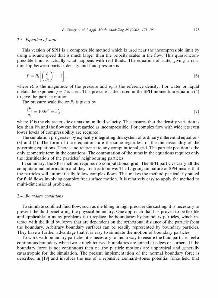
The C-shaped mould is geometrically simple, enabling its initial set-up to be built by hand. Thesimple geometry also allows any programming problem that is associated with the geometry to beidentified relatively more readily. Furthermore, it allows easier capture of ‘‘clean’’ experimentalimages from water analogue modelling. The second die is more representative of industrial andengineering casting objects. It is a testing example for our methodology for constructing the initialset-up for a SPH simulation.

4.1. C-shaped mould

Fig. 1 shows the geometry of the die used in previous experimental and numerical simulations[3,8]. It was 50 mm long, 20.9 mm high and 20 mm deep. It is connected to the runner by a gate ofwidth 2.9 mm. The width of the vertical sections was 4 mm and the width of the connectinghorizontal section was 4.9 mm.

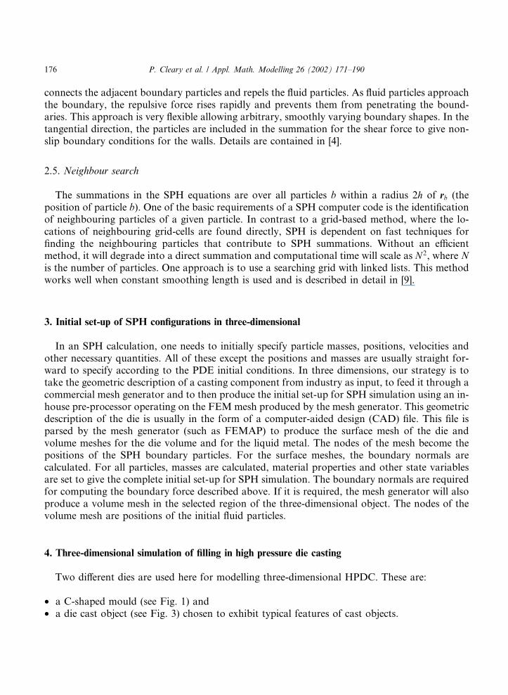
A resolution of 2.6 particles per millimetre was used giving a total of 208,054 particles forthe simulation. This resolution is chosen based on our two-dimensional studies on the effects ofresolution on die filling [3]. Lower and higher resolutions do not change the filling pattern. Thefluid speed through the gate was 0.62 m/s. Two perspective views of the filling pattern at sixdifferent times are shown in Fig. 2. The fluid particles are shown coloured by their speed.

The flow in the xy-plane was broadly similar to that predicted by the two-dimensional SPHsimulation and observed in the matching experiments [8]. In particular, the separation from theright angle bends and the back filling down the left side of the first vertical section are reproduced.

Concentrating on the flow after 28 ms when the horizontal section of the die cavity was be-ginning to be filled, the two views show the highly fragmented nature of the fluid and the three-dimensionality of the fluid flow pattern. These features continue as the die cavity is increasinglyfilled, with many voids in the fluid. These voids move in an irregular and complex pattern andwould lead to significant porosity in the final cast component.

4.2. Die cast object

The geometry of the die, the gate, the runner and the cylindrical plunger section is shown in Fig.3. In real die casting, the cylinder orientation would be horizontal and the part vertical but for themodelling we use a reference orientation as shown here. The fluid initially fills the cylindricalcolumn and was pushed downward by a plunger at the top of the fluid moving at 15 m/s. In thesimulation, a resolution of 1 particle per millimetre was used giving a total of 243,576 particles.These SPH simulations took about 3.5 days on a single 677 MHz processor of an Alpha ES40.

Fig. 1. Cross-section of the three-dimensional C-shaped HPDC die.

P. Cleary et al. / Appl. Math. Modelling 26 (2002) 171–190 177

Fig. 2. Two perspective views of the filling of the C-shaped mould. The particles are coloured by velocity with red being

60 m/s and dark blue being stationary. Left: xy-plane. Right: xz-plane.

178 P. Cleary et al. / Appl. Math. Modelling 26 (2002) 171–190

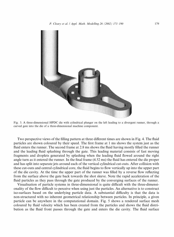
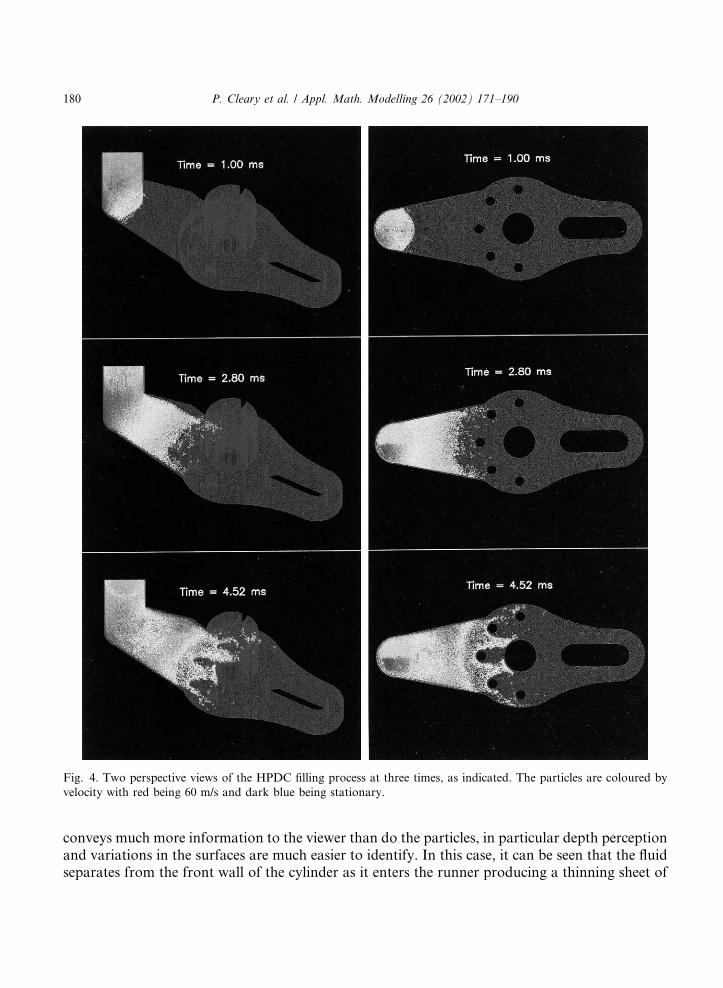
Two perspective views of the filling pattern at three different times are shown in Fig. 4. The fluidparticles are shown coloured by their speed. The first frame at 1 ms shows the system just as thefluid enters the runner. The second frame at 2.8 ms shows the fluid having mostly filled the runnerand the leading fluid splashing through the gate. This leading material consists of fast movingfragments and droplets generated by splashing when the leading fluid flowed around the rightangle turn as it entered the runner. In the final frame (4.52 ms) the fluid has entered the die properand has split into separate jets around each of the vertical cylindrical cut-outs. After collision withthese cut-outs and central cylindrical core, the fluid begins to flow vertically up into the upper partof the die cavity. At the time the upper part of the runner was filled by a reverse flow reflectingfrom the surface above the gate back towards the shot sleeve. Note the rapid acceleration of thefluid particles as they pass through the gate produced by the converging surfaces of the runner.

Visualisation of particle systems in three-dimensional is quite difficult with the three-dimensi-onality of the flow difficult to perceive when using just the particles. An alternative is to constructiso-surfaces based on the underlying particle data. A substantial difficulty is that the data isnon-structured with no inherent geometrical relationship between particles. In principle, a givenparticle can be anywhere in the computational domain. Fig. 5 shows a rendered surface meshcoloured by fluid velocity which has been created from the particles and shows the fluid distri-bution as the fluid front passes through the gate and enters the die cavity. The fluid surface

Fig. 3. A three-dimensional HPDC die with cylindrical plunger on the left leading to a divergent runner, through a

curved gate into the die of a three-dimensional machine component.

P. Cleary et al. / Appl. Math. Modelling 26 (2002) 171–190 179

conveys much more information to the viewer than do the particles, in particular depth perceptionand variations in the surfaces are much easier to identify. In this case, it can be seen that the fluidseparates from the front wall of the cylinder as it enters the runner producing a thinning sheet of

Fig. 4. Two perspective views of the HPDC filling process at three times, as indicated. The particles are coloured by

velocity with red being 60 m/s and dark blue being stationary.

180 P. Cleary et al. / Appl. Math. Modelling 26 (2002) 171–190

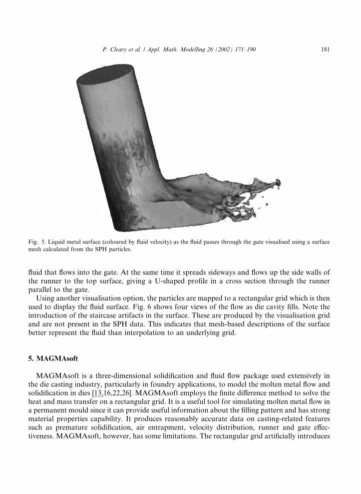
fluid that flows into the gate. At the same time it spreads sideways and flows up the side walls ofthe runner to the top surface, giving a U-shaped profile in a cross section through the runnerparallel to the gate.

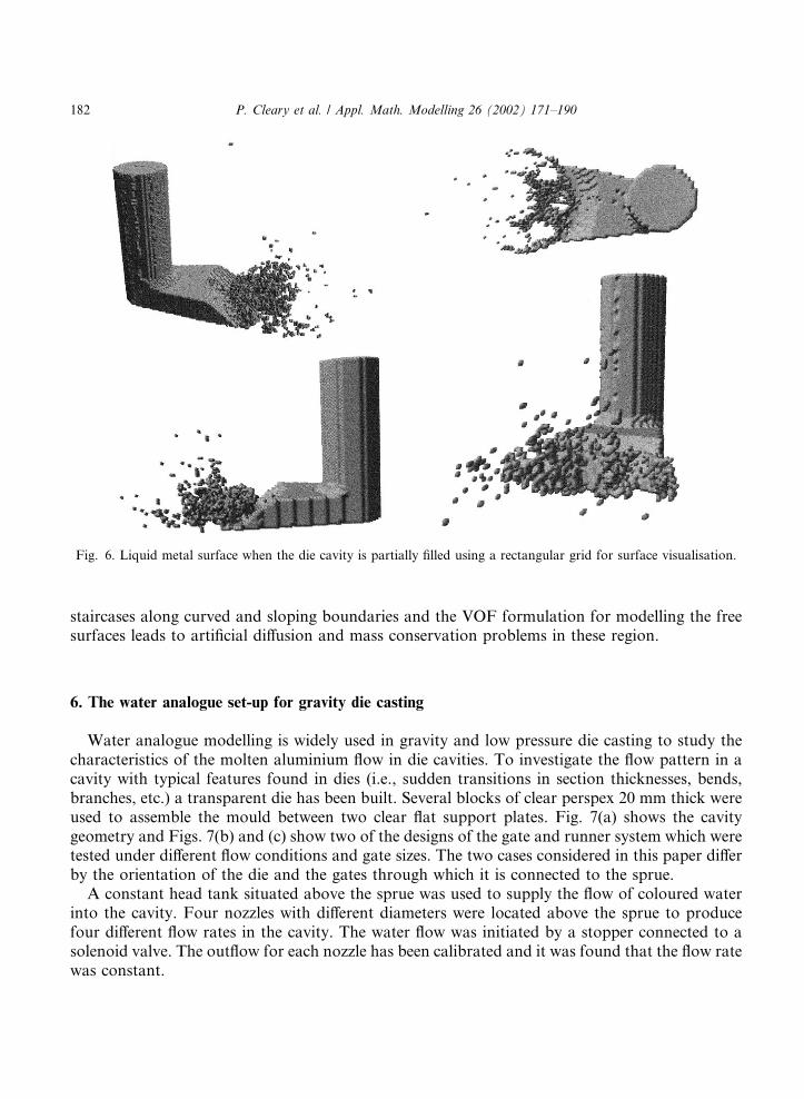
Using another visualisation option, the particles are mapped to a rectangular grid which is thenused to display the fluid surface. Fig. 6 shows four views of the flow as die cavity fills. Note theintroduction of the staircase artifacts in the surface. These are produced by the visualisation gridand are not present in the SPH data. This indicates that mesh-based descriptions of the surfacebetter represent the fluid than interpolation to an underlying grid.

5. MAGMAsoft

MAGMAsoft is a three-dimensional solidification and fluid flow package used extensively inthe die casting industry, particularly in foundry applications, to model the molten metal flow andsolidification in dies [13,16,22,26]. MAGMAsoft employs the finite difference method to solve theheat and mass transfer on a rectangular grid. It is a useful tool for simulating molten metal flow ina permanent mould since it can provide useful information about the filling pattern and has strongmaterial properties capability. It produces reasonably accurate data on casting-related featuressuch as premature solidification, air entrapment, velocity distribution, runner and gate effec-tiveness. MAGMAsoft, however, has some limitations. The rectangular grid artificially introduces

Fig. 5. Liquid metal surface (coloured by fluid velocity) as the fluid passes through the gate visualised using a surface

mesh calculated from the SPH particles.

P. Cleary et al. / Appl. Math. Modelling 26 (2002) 171–190 181

staircases along curved and sloping boundaries and the VOF formulation for modelling the freesurfaces leads to artificial diffusion and mass conservation problems in these region.

6. The water analogue set-up for gravity die casting

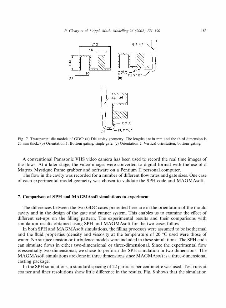
Water analogue modelling is widely used in gravity and low pressure die casting to study thecharacteristics of the molten aluminium flow in die cavities. To investigate the flow pattern in acavity with typical features found in dies (i.e., sudden transitions in section thicknesses, bends,branches, etc.) a transparent die has been built. Several blocks of clear perspex 20 mm thick wereused to assemble the mould between two clear flat support plates. Fig. 7(a) shows the cavitygeometry and Figs. 7(b) and (c) show two of the designs of the gate and runner system which weretested under different flow conditions and gate sizes. The two cases considered in this paper differby the orientation of the die and the gates through which it is connected to the sprue.

A constant head tank situated above the sprue was used to supply the flow of coloured waterinto the cavity. Four nozzles with different diameters were located above the sprue to producefour different flow rates in the cavity. The water flow was initiated by a stopper connected to asolenoid valve. The outflow for each nozzle has been calibrated and it was found that the flow ratewas constant.

Fig. 6. Liquid metal surface when the die cavity is partially filled using a rectangular grid for surface visualisation.

182 P. Cleary et al. / Appl. Math. Modelling 26 (2002) 171–190

A conventional Panasonic VHS video camera has been used to record the real time images ofthe flows. At a later stage, the video images were converted to digital format with the use of aMatrox Mystique frame grabber and software on a Pentium II personal computer.

The flow in the cavity was recorded for a number of different flow rates and gate sizes. One caseof each experimental model geometry was chosen to validate the SPH code and MAGMAsoft.

7. Comparison of SPH and MAGMAsoft simulations to experiment

The differences between the two GDC cases presented here are in the orientation of the mouldcavity and in the design of the gate and runner system. This enables us to examine the effect ofdifferent set-ups on the filling pattern. The experimental results and their comparisons withsimulation results obtained using SPH and MAGMAsoft for the two cases follow.

In both SPH and MAGMAsoft simulations, the filling processes were assumed to be isothermaland the fluid properties (density and viscosity at the temperature of 20 �C used were those ofwater. No surface tension or turbulence models were included in these simulations. The SPH codecan simulate flows in either two-dimensional or three-dimensional. Since the experimental flowis essentially two-dimensional, we chose to perform the SPH simulation in two dimensions. TheMAGMAsoft simulations are done in three dimensions since MAGMAsoft is a three-dimensionalcasting package.

In the SPH simulations, a standard spacing of 22 particles per centimetre was used. Test runs atcoarser and finer resolutions show little difference in the results. Fig. 8 shows that the simulation

Fig. 7. Transparent die models of GDC: (a) Die cavity geometry. The lengths are in mm and the third dimension is

20 mm thick. (b) Orientation 1: Bottom gating, single gate. (c) Orientation 2: Vertical orientation, bottom gating.

P. Cleary et al. / Appl. Math. Modelling 26 (2002) 171–190 183

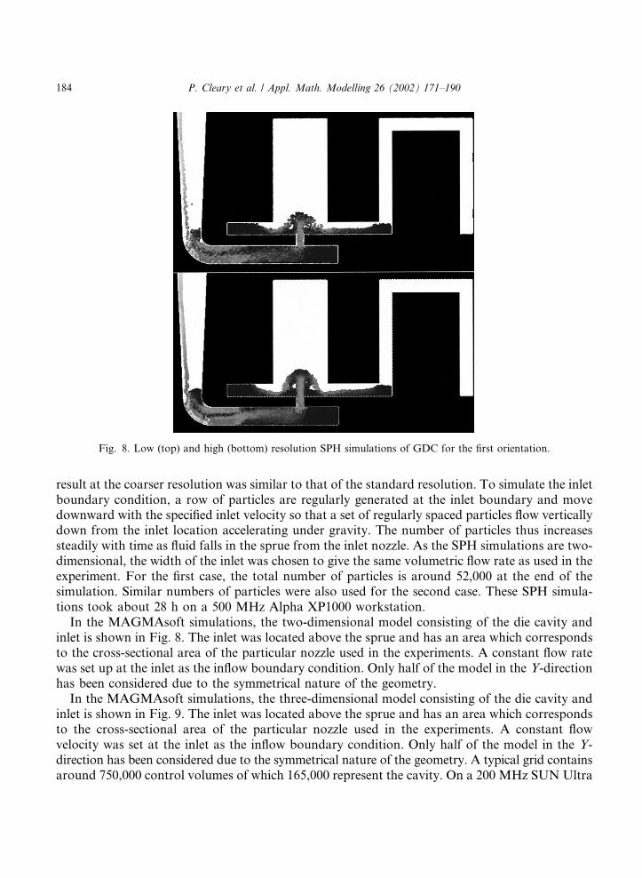
result at the coarser resolution was similar to that of the standard resolution. To simulate the inletboundary condition, a row of particles are regularly generated at the inlet boundary and movedownward with the specified inlet velocity so that a set of regularly spaced particles flow verticallydown from the inlet location accelerating under gravity. The number of particles thus increasessteadily with time as fluid falls in the sprue from the inlet nozzle. As the SPH simulations are two-dimensional, the width of the inlet was chosen to give the same volumetric flow rate as used in theexperiment. For the first case, the total number of particles is around 52,000 at the end of thesimulation. Similar numbers of particles were also used for the second case. These SPH simula-tions took about 28 h on a 500 MHz Alpha XP1000 workstation.

In the MAGMAsoft simulations, the two-dimensional model consisting of the die cavity andinlet is shown in Fig. 8. The inlet was located above the sprue and has an area which correspondsto the cross-sectional area of the particular nozzle used in the experiments. A constant flow ratewas set up at the inlet as the inflow boundary condition. Only half of the model in the Y-directionhas been considered due to the symmetrical nature of the geometry.

In the MAGMAsoft simulations, the three-dimensional model consisting of the die cavity andinlet is shown in Fig. 9. The inlet was located above the sprue and has an area which correspondsto the cross-sectional area of the particular nozzle used in the experiments. A constant flowvelocity was set at the inlet as the inflow boundary condition. Only half of the model in the Y-direction has been considered due to the symmetrical nature of the geometry. A typical grid containsaround 750,000 control volumes of which 165,000 represent the cavity. On a 200 MHz SUN Ultra

Fig. 8. Low (top) and high (bottom) resolution SPH simulations of GDC for the first orientation.

184 P. Cleary et al. / Appl. Math. Modelling 26 (2002) 171–190

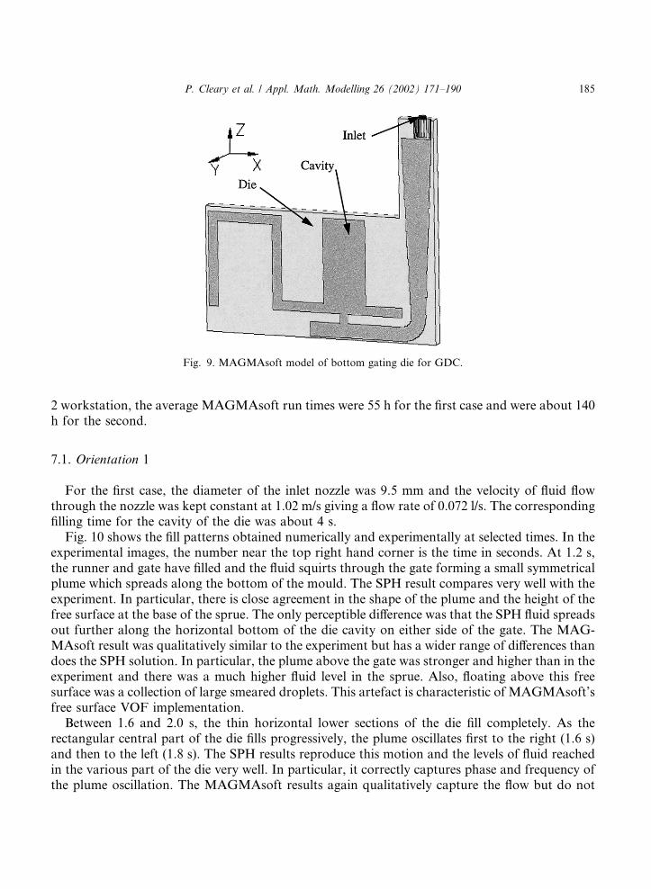
2 workstation, the average MAGMAsoft run times were 55 h for the first case and were about 140h for the second.

7.1. Orientation 1

For the first case, the diameter of the inlet nozzle was 9.5 mm and the velocity of fluid flowthrough the nozzle was kept constant at 1.02 m/s giving a flow rate of 0.072 l/s. The correspondingfilling time for the cavity of the die was about 4 s.

Fig. 10 shows the fill patterns obtained numerically and experimentally at selected times. In theexperimental images, the number near the top right hand corner is the time in seconds. At 1.2 s,the runner and gate have filled and the fluid squirts through the gate forming a small symmetricalplume which spreads along the bottom of the mould. The SPH result compares very well with theexperiment. In particular, there is close agreement in the shape of the plume and the height of thefree surface at the base of the sprue. The only perceptible difference was that the SPH fluid spreadsout further along the horizontal bottom of the die cavity on either side of the gate. The MAG-MAsoft result was qualitatively similar to the experiment but has a wider range of differences thandoes the SPH solution. In particular, the plume above the gate was stronger and higher than in theexperiment and there was a much higher fluid level in the sprue. Also, floating above this freesurface was a collection of large smeared droplets. This artefact is characteristic of MAGMAsoft’sfree surface VOF implementation.

Between 1.6 and 2.0 s, the thin horizontal lower sections of the die fill completely. As therectangular central part of the die fills progressively, the plume oscillates first to the right (1.6 s)and then to the left (1.8 s). The SPH results reproduce this motion and the levels of fluid reachedin the various part of the die very well. In particular, it correctly captures phase and frequency ofthe plume oscillation. The MAGMAsoft results again qualitatively capture the flow but do not

Fig. 9. MAGMAsoft model of bottom gating die for GDC.

P. Cleary et al. / Appl. Math. Modelling 26 (2002) 171–190 185

quite capture the complete filling of the horizontal sections (1.6 and 1.8 s). The fine details of theplume structure and motion are also not quite captured.

Fig. 10. Filling of GDC die in the first orientation: MAGMAsoft (left), water analogue (middle) and SPH (right).

186 P. Cleary et al. / Appl. Math. Modelling 26 (2002) 171–190

As the amount of fill increases, the sloshing motion in the rectangular section of the cavity wasincreasingly dampened down and the free surfaces become increasingly flat. Both the SPH andMAGMAsoft simulation results reproduce the later stages of the filling well. However, theMAGMAsoft result shows a lower fluid level in the sprue than the experiment. By 3.4 s, therectangular section above the gate was completely filled and the horizontal section of the C-shaped cavity to the right was beginning to fill. This was reproduced very nicely by both SPH andMAGMAsoft solutions. The SPH simulation slightly over-predicts the height of water in thesprue whereas the MAGMAsoft result slightly under-predicts this level.

7.2. Orientation 2

Fig. 7(c) shows the geometry for the second die orientation. The diameter of the inlet nozzlewas 6.9 mm and the velocity of fluid flow through the nozzle was kept constant at 1.12 m/s givinga flow rate of 0.042 l/s. The filling time for the cavity of the die was about 8.5 s.

In Fig. 11, the fill patterns obtained numerically and experimentally at selected time instancesare compared. In the experimental images, the number at the bottom left corner is the time inseconds. The filling process for the second case was somewhat similar to that of the first in that theearly part of die filling was dominated by sloshing free surface wave motion. This sloshing motionwas damped after a certain time. We thus restrict our discussion to the early part of the die fillingwhen the process was much more dynamic.

At 1.6 s, the large rectangular section of the cavity was just starting to fill. Both the MAG-MAsoft and SPH simulation results reproduce this well. The shape of the fluid front was wellpredicted by the SPH simulation but less well by the MAGMAsoft simulation. The MAGMAsoftresult shows a lower fluid level in the sprue than that of the experimental result, while the SPHresult shows a marginally higher level than the experiment. Both methods have some minorproblems with jet stability near the free surface in the sprue at this stage.

At 2.1 s, the front of the fluid almost reaches the left wall of the rectangular section of the diecavity. The SPH simulation predicts the overall height of the fluid and the closeness of the fluidfront to the left wall very well. In particular, it was able to capture the fine details of the shape ofthe free surface where the upward jet entering the die slumps under gravity to give the steppedprofile observed. The MAGMAsoft simulation under-predicts the level of fill and the closeness ofthe fluid front to the left wall. MAGMAsoft qualitatively reproduces the elevation of the fluidsurface near the right wall of the rectangular section. The simulation results show the slight underprediction by MAGMAsoft and over prediction by SPH of the fluid level in the sprue.

At 2.2 s, the fluid shows a surface wave having just reflected off the left wall of the rectangularsection of the cavity. The wave was the result of the original wave of fluid travelling to the lefthitting the left wall and returning to the right. The upward motion of the fluid from the verticalsection above the gate still has sufficient momentum to maintain the elevated surface mentionedabove. The SPH solution captures this free surface remarkably well, while the MAGMAsoft resultshows the fluid has just reached the left wall.

At 2.4 s, the left half of the free surface in the rectangular section has become flat as the freesurface wave from the left moves further back to the right. SPH again reproduces the shape of thefree surface of the fluid very well. The MAGMAsoft result was just beginning to show motion ofthe wave from the left at this stage. However, it predicts the fluid level in the sprue better than

P. Cleary et al. / Appl. Math. Modelling 26 (2002) 171–190 187

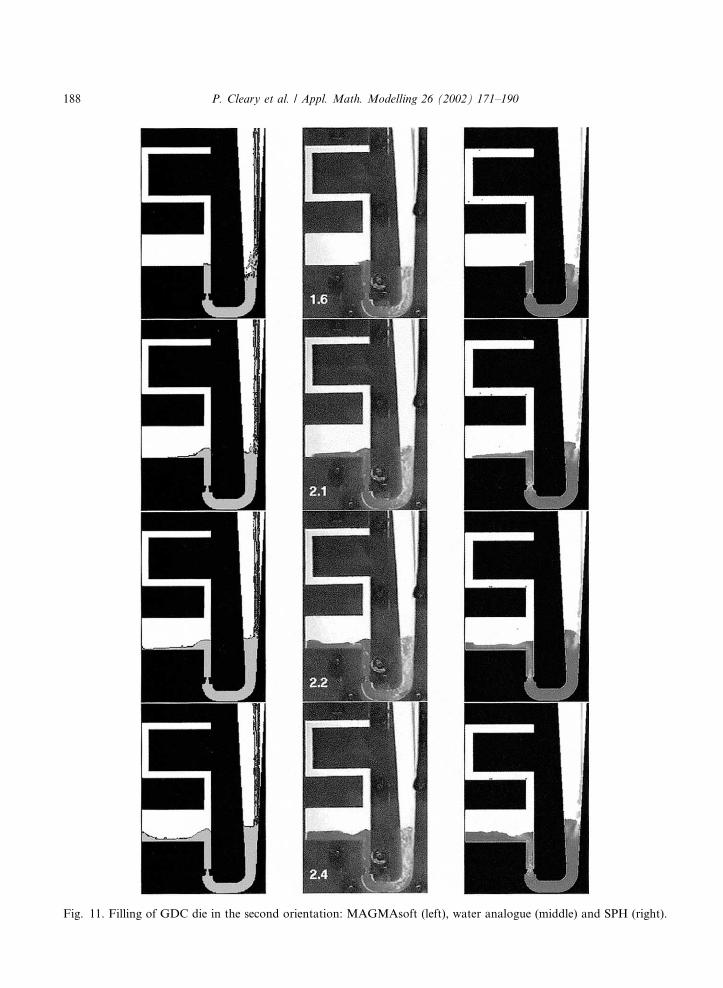
Fig. 11. Filling of GDC die in the second orientation: MAGMAsoft (left), water analogue (middle) and SPH (right).

188 P. Cleary et al. / Appl. Math. Modelling 26 (2002) 171–190

SPH does. Soon after 2.4 s, the fluid surface loses its wave-like structure and flattens out. BothMAGMAsoft and SPH simulations reproduce this feature well.

8. Conclusion

In this paper, we have described the SPH method and the application of SPH to simulate thethree-dimensional die filling in high pressure die casting. The methodology for three-dimensionalindustrial SPH modelling involves the CAD specification of die geometry, the construction ofFEM meshes using commercial mesh generators and the conversion of this to SPH input data.The difficulty associated with visualisation of complex three-dimensional free surface flows usingnon-structured particle data were also highlighted.

Two examples demonstrate the complex three-dimensional flow patterns in the HPDC fillingprocess. The complex free surface behaviour including splashing and surface breakup is handlednaturally by SPH. This results from the Lagrangian nature of SPH and the superior mass con-servation properties of this particle method. This is due to the ease of advection of small dropletsthrough space by SPH which is automatic and fully conservative whereas such advection throughan Eulerian grid can be numerically diffusive.

SPH and MAGMAsoft simulations of GDC for a complex die with two different orientationshas also been presented. These were compared to matching experiments. The agreement withGDC experiment is good for both numerical methods, with each being able to predict theoverall structure of the filling process. In general, the natural free surface capability of SPH allowsit to better capture the free surface wave behaviour and the fine details of the flow. Conversely,MAGMAsoft generally predicts the level of the fluid in the sprue slightly better.

Acknowledgements

This project is funded by the Cooperative Research Centre for Cast Metals Manufacturing(CAST).

References

[1] P.W. Cleary, Modelling confined multi-material heat and mass flows using SPH, Appl. Math. Modell. 22 (1998)

981–993.

[2] P.W. Cleary, J. Ha, SPH modelling of isothermal high pressure die casting, in: Proceedings of the 13th Australasian

Fluid Mechanics Conference, Melbourne, Australia, December 1998, pp. 663–666.

[3] P.W. Cleary, J. Ha, V. Ahuja, High pressure die casting using smoothed particle hydrodynamics, Int. J. Cast Metal

Res. (2000) 335–355.

[4] P.W. Cleary, J.J. Monaghan, Boundary interactions and transition to turbulence for standard CFD problems using

SPH, in: D. Stewart, H. Gardener, D. Singleton (Eds.), Proceedings of the 6th International Computational

Techniques and Applications Conference, Canberra, ACT, 1993, p. 157.

[5] S.J. Cummins, M. Rudman, An SPH projection method, J. Comp. Phys. 152 (1999) 584–607.

[6] A.J. Davis, S.J. Asquith, Water analogue studies of fluid flow in the die casting process, in: Trans. 13th Congress,

Milwaukee, USA, Paper G-T85-063, 1985.

P. Cleary et al. / Appl. Math. Modelling 26 (2002) 171–190 189

[7] J. Ha, P. Cleary, Comparison of SPH simulations of high pressure die casting with the experiments and VOF

simulations of Schmid and Klein, Int. J. Cast Metals Res. (2000), in press.

[8] J. Ha, P. Cleary, V. Ahuja, Comparison of SPH simulation of high speed die filling with experiment, in:

Proceedings of the 13th Australasian Fluid Mechanics Conference, Melbourne, Australia, December 1998, pp.

901–904.

[9] R.W. Hockney, J.W. Eastwood, Computer Simulation Using Particles, Institute of Physics Publishing Ltd, 1988.

[10] C.W. Hirt, B.D. Nichols, Volume of fluid method for the dynamics of free boundaries, J. Comp. Phys. 39 (1981)

201–225.

[11] W-S. Hwang, R.A. Stoehr, Modelling fluid flow, Metals Handbook, Casting, ASM Int. 15 (1988) 867–876.

[12] L.R. Jai, S.M. Xiong, B.C. Lui, Mold filling and heat transfer simulation of die casting process, in: P.R. Sahm,

P.N. Hansen, J.G. Conley (Eds.), Modeling of Casting, Welding and Advanced Solidification Processes IX,

Aachen, Germany, 1998, pp. 303–310.

[13] M.R. Jolly, H.S.H. Lo, M. Turan, X. Yang, J. Campbell, Development of practical quiescent running systems

without foam filters for use in aluminium castings using computer modelling, in: P.R. Sahm, P.N. Hansen, J.G.

Conley (Eds.), Modeling of Casting, Welding and Advanced Solidification Processes IX, Aachen, Germany, 2000,

pp. 311–318.

[14] D. Kothe, D. Juric, K. Lam, B. Lally, Numerical recipes for mold filling simulation, in: B.G. Thomas, C.

Beckermann (Eds.), Modeling of Casting, Welding and Advanced Solidification Processes VIII, San Diego, CA,

1998, pp. 17–28.

[15] Y.C. Lee, H.Y. Hwang, J.K. Choi, A study on the application of solidification and fluid flow simulation to die

design in gravity die casting, in: P.R. Sahm, P.N. Hansen, J.G. Conley (Eds.), Modeling of Casting, Welding and

Advanced Solidification Processes IX, Aachen, Germany, 2000, pp. 349–356.

[16] MAGMAsoft User Manual MAGMA GmbH, Kackertstrasse 11, D-52072, Aachen, Germany, 1996.

[17] J.J. Monaghan, Smoothed particle hydrodynamics, Ann. Rev. Astron. Astrophys. 30 (1992) 543–574.

[18] J.J. Monaghan, Simulating free surface flows with SPH, J. Comp. Phys. 110 (1994) 399–406.

[19] J.J. Monaghan, Improved modelling of boundaries, SPH Technical Note #2, CSIRO Division of Mathematics and

Statistics, Technical Report DMS – C 95/86, 1995.

[20] J.P. Morris, P.J. Fox, Y. Zhu, Modeling low Reynolds number incompressible flows using SPH, J. Comput. Phys.

136 (1997) 214–226.

[21] J.P. Morris, Simulating surface tension with smoothed particle hydrodynamics, Int. J. Numer. Meth. Fluids 33

(2000) 333–353.

[22] F. Scheppe, P.R. Sahm, W. Hermann, U. Paul, J. Preuhs, Comparison of the numerical simulation and the cast

process of nickel aluminides, in: P.R. Sahm, P.N. Hansen, J.G. Conley (Eds.), Modeling of Casting, Welding and

Advanced Solidification Processes IX, Aachen, Germany, 2000, pp. 207–214.

[23] M. Schmid, F. Klein, Experimental investigation of mold filling in high pressure die casting, in: B.G. Thomas, C.

Beckermann (Eds.), Modeling of Casting, Welding and Advanced Solidification Processes VIII, San Diego, CA,

1998, pp. 1131–1136.

[24] M.C. Schneider, C. Beckermann, D.M. Lipinski, W. Schaefer, Macrosegregation formation during solidification of

complex steel castings: three-dimensional numerical simulation and experimental comparison, in: P.R. Sahm, P.N.

Hansen, J.G. Conley (Eds.), Modeling of Casting, Welding and Advanced Solidification Processes IX, Aachen,

Germany, 2000, pp. 257–264.

[25] J.E. Welch, F.H. Harlow, The MAC method, a computing technique for solving incompressible, transient fluid

flow problems involving free surface, Phys. Fluids 9 (1966) 842–851.

[26] M. Wu, M. Augthun, I. Wagner, J. Sch€aadlich-Stubenrauch, P.R. Sahm, Integration of numerical simulation and

rapid prototyping for investment castings, in: P.R. Sahm, P.N. Hansen, J.G. Conley (Eds.), Modeling of Casting,

Welding and Advanced Solidification Processes IX, Aachen, Germany, 2000, pp. 278–285.

[27] Z.A. Xu, Using a dynamic domain decomposition algorithm to parallelize a mould filling calculation, in: P.R.

Sahm, P.N. Hansen, J.G. Conley (Eds.), Modeling of Casting, Welding and Advanced Solidification Processes IX,

Aachen, Germany, 2000, pp. 312–319.

190 P. Cleary et al. / Appl. Math. Modelling 26 (2002) 171–190