Research Article

GD-RDA:

A New Regularized Discriminant

Analysis for High-Dimensional Data

YAN ZHOU,1 BAOXUE ZHANG,2 GAORONG LI,3 TIEJUN TONG,4 and XIANG WAN5

ABSTRACT

High-throughput techniques bring novel tools and also statistical challenges to genomicresearch. Identification of which type of diseases a new patient belongs to has been recog-nized as an important problem. For high-dimensional small sample size data, the classicaldiscriminant methods suffer from the singularity problem and are, therefore, no longerapplicable in practice. In this article, we propose a geometric diagonalization method for theregularized discriminant analysis. We then consider a bias correction to further improve theproposed method. Simulation studies show that the proposed method performs better than,or at least as well as, the existing methods in a wide range of settings. A microarray datasetand an RNA-seq dataset are also analyzed and they demonstrate the superiority of theproposed method over the existing competitors, especially when the number of samplesis small or the number of genes is large. Finally, we have developed an R package called‘‘GDRDA’’ which is available upon request.

Keywords: bias correction, classification, diagonalization, discriminant, geometric, microarray,

RNA-seq.

1. INTRODUCTION

H igh-throughput techniques allow us to acquire thousands of or more gene expression values

simultaneously, which introduces novel approaches to genomic research. One important goal of ana-

lyzing gene expression microarray data is to identify which type of diseases a new patient belongs to. The

same problem also applies to the RNA-seq data, which are getting more popular in genomic research and that

use next-generation sequencing to quantify gene expression levels (Mardis, 2008; Morozova et al., 2009;

Wang et al., 2009). For such classification problems, the discriminant methods are often popular in practice,

including the linear discriminant analysis (LDA) and the quadratic discriminant analysis (QDA). These

methods perform well when the number of samples, n, is large and the number of genes, p, is small.

For microarray data, the number of samples is usually small compared with the number of genes. It is not

even uncommon to see microarray data with less than ten samples (Kaur et al., 2012; Mokry et al., 2012;

1College of Mathematics and Statistics, Institute of Statistical Sciences, Shenzhen University, ShenZhen, China.2School of Statistics, Capital University of Economics and Business, Beijing, China.3Beijing Institute for Scientific and Engineering Computing, Beijing University of Technology, Beijing, China.Departments of 4Mathematics and 5Computer Science, Hong Kong Baptist University, Hong Kong, China.

JOURNAL OF COMPUTATIONAL BIOLOGY

Volume 24, Number 0, 2017

# Mary Ann Liebert, Inc.

Pp. 1–13

DOI: 10.1089/cmb.2017.0029

1

Searcy et al., 2012). In such situations, the classical LDA and QDA are no longer applicable in practice

since the sample covariance matrices are singular. Guo et al. (2007) proposed a regularized LDA for high-

dimensional small sample size data. We note, however, that this approach is often unstable when n is

relatively small or the ratio of p=n is relatively large.

In 2002, Dudoit et al. introduced a diagonalization method for LDA and QDA, which leads to the well-

known diagonal linear discriminant analysis (DLDA) and the diagonal quadratic discriminant analysis

(DQDA), respectively. By simulation studies, they demonstrated the superiority of DLDA and DQDA over

more sophisticated methods for classification of microarray data. Bickel and Levina (2004) also pointed out

that if the estimated correlations are all very noisy, then it is better off without estimating them. In addition,

Lee et al. (2005) observed that the discriminant rules with an inverse generalized matrix may not perform

as well as the diagonal discriminant rules for microarray data. Thereafter, the diagonal covariance matrix

assumption has been widely applied for high-dimensional small sample size data. Apart from this direction,

Friedman (1989) has proposed a regularization method to further improve the performance of LDA and

QDA when the sample size is not sufficiently large compared with the dimension. Specifically, they shrunk

the individual sample covariance matrix toward the pooled sample covariance matrix, and referred to the

final rule as the regularized discriminant analysis (RDA).

To our knowledge, there is little work in the literature that is specifically designed for a diagonalization

method for RDA, in cases when n is relatively small or p is relatively large so that RDA may not perform

well by itself. Following the spirit of diagonalization, in this article, we propose a diagonalized version for

RDA. The new method consists of two main steps: the diagonalization step and the bias correction step. For

the diagonalization step, instead of the arithmetic mean, we apply the geometric mean to form a geometric

diagonalization (GD) method for RDA. For the bias correction step, we propose an unbiased estimator for

the diagonalized discriminant score to further improve the performance in the unbalanced designs. In

addition, we apply the class-weighted accuracy (CWA) criterion, which was introduced in Cohen et al.

(2006), to measure the prediction accuracy of the proposed method. Simulation results show that our

proposed method performs better than, or at least as well as, the existing competitors in a wide range of

settings. A microarray dataset and an RNA-seq dataset are also analyzed, and they all demonstrate the

advantage of the proposed GD method for RDA.

The remainder of the article is organized as follows. In Section 2, we first give a brief description of

RDA and then propose our GD method for RDA. In Section 3, we propose a bias correction method for the

proposed discriminant score and also introduce the CWA criterion for assessment. Simulation studies and

real-data analysis are conducted and analyzed in Sections 4 and 5, respectively. Finally, we conclude the

article in Section 6 and provide the technical proofs in the Appendix.

2. METHODS

2.1. Regularized discriminant analysis

Let K be the number of classes, and the samples be randomly drawn from a p-dimensional multivari-

ate normal distribution with mean vector lk = (lk1‚ . . . ‚ lkp)T and covariance matrix Sk for each class, where

k = 1‚ . . . ‚ K. Specifically, there are nk independent and identically distributed (i.i.d.) samples in the kth class,

xk‚ 1‚ . . . ‚ xk‚ nk*i:i:d:MVN(lk‚Sk): (2:1)

Let n =PK

k = 1 nk be the total number of samples for all classes. Given a new observation, y, the goal of

classification is to predict which class label the observed y belongs to. Let also pk be the proportion of

observing a sample from the kth class. Throughout the article, we set pk = nk=n so thatPK

k = 1 pk = 1.

The QDA decision rule is to assign y to the class with label arg minkdQk (y), where dQ

k (y) is the dis-

criminant score defined as

dQk (y) = (y - lk)TS - 1

k (y - lk) + ln jSkj - 2 ln pk:

Note that the population parameters in the score just provided are unknown and need to be estimated

from the sample data. Let �xk =Pnk

i = 1 xk‚ i=nk be the sample means, and Sk =Pnk

i = 1 (xk‚ i - �xk)(xk‚ i - �xk)T=(nk - 1) be the sample covariance matrices. By replacing the unknown parameters (lk‚Sk) with their sample

estimates (�xk‚ Sk), we have the sample version of dQk (y) as

2 ZHOU ET AL.

dQk (y) = (y - �xk)T S - 1

k (y - �xk) + ln jSkj - 2 ln pk: (2:2)

If we further assume that the covariance matrices are all the same, that is, Sk =S for all k, and estimate

the common S by the pooled sample covariance matrix Spool =PK

k = 1 (nk - 1)Sk=(n - K), then it leads to the

sample version of LDA with the discriminant score defined as

dLk (y) = (y - �xk)T S - 1

pool(y - �xk) - 2 ln pk: (2:3)

As shown in Friedman (1989), QDA and LDA usually perform well when the data follow a multivariate

normal distribution and when the sample size is large compared with the dimension. In particular, QDA

requires nk � p to ensure Sk are nonsingular, and LDA requires n � p to ensure Spool is nonsingular. These

requirements have largely limited the application of QDA and LDA for classifying high-dimensional small

sample size data.

To improve the existing literature, Friedman (1989) considered a regularization method for the dis-

criminant analysis. Specifically, he proposed to estimate Sk by

Sk(k) = (1 - k)Sk + kSpool‚ (2:4)

where k is a regularization parameter with 0 � k � 1. It controls the degree of shrinkage of the class-specific

sample covariance matrix toward the pooled sample covariance matrix. When k = 0, it provides no shrinkage

and yields QDA. When k = 1, it shrinks fully to the pooled sample covariance matrix and yields LDA. Noting

that the regularized estimator (in 2.4) may not provide enough regularization, Friedman (1989) had also

considered a second-step regularization that shrinks Sk(k) (in 2.4) toward a multiple of the identity matrix:

Sk(k‚ c) = (1 - c)Sk(k) + c[tr(Sk(k))=p]I‚ (2:5)

where tr(�) is the trace of the matrix, I is the identity matrix, and c is an additional regularization parameter

with 0 � c � 1.

Given the value of k, the additional parameter c controls the degree of shrinkage toward the multiple of

the identity matrix. Recall that the multiplier tr(Sk(k))=p is the same as the average eigenvalue of Sk(k).

The second-step regularization, therefore, has the effect of decreasing the possibly over-estimated large

eigenvalues and increasing the possibly under-estimated small eigenvalues. The regularized estimator

Sk(k‚ c) provides a two-parameter family of estimators for the class-specific covariance matrix. With this

estimator, the regularized discriminant score is

dRk (y) = (y - �xk)T [Sk(k‚ c)] - 1(y - �xk) + ln jSk(k‚ c)j - 2 ln pk: (2:6)

Accordingly, we refer to this classification method as RDA. Owing to the two parameters (k‚ c)‚ RDA

provides a fairly rich class of regularization alternative rules. For instance, the lower left corner with

(k = 0‚ c = 0) represents QDA, the lower right corner with (k = 1‚ c = 0) represents LDA, and the upper right

corner with (k = 1‚ c = 1)represents the nearest neighbor classifier. In addition, fixing c at 0 and varying kproduces a discriminant rule between QDA and LDA; fixing k at 0 and varying c yields a ridge-type analog

of QDA; and fixing k at 1 and varying c yields a ridge-type analog of LDA.

2.2. A diagonalization method for RDA

For high-dimensional data such as microarrays, the dimension can be much larger than the sample size.

In such situations, QDA and LDA are no longer applicable since the sample covariance matrices are

singular. In contrast, the regularized discriminant methods, including RDA and its variants, may still work

if the parameters k and c are taken appropriately. For instance, Guo et al. (2007) proposed a regularized

LDA for high-dimensional small sample size data, which is essentially a special case of RDA with k fixed

at 1. Nevertheless, these approaches are usually unstable when n is relatively small or the ratio of p=n is

relatively large.

To overcome the singularity problem in discriminant analysis, Dudoit et al. (2002) introduced a diag-

onalization method for LDA and QDA. Let Dk = diag(s2k1‚ . . . ‚ s2

kp) be the diagonal matrix of the sample

covariance matrix Sk, and Dpool = diag(s21‚ . . . ‚ s2

p) be the diagonal matrix of the pooled covariance matrix

Spool. Given that a diagonal matrix is always invertible, Dudoit et al. (2002) replaced Sk by Dk (in 2.2) and

formed the DQDA, with the discriminant score defined as

GD-RDA 3

dQk (y) =

Xp

i = 1

(yi - �xki)2=s2

ki +Xp

i = 1

ln s2ki - 2 ln pk: (2:7)

Similarly, DLDA was formed by replacing Spool by Dpool (in 2.3), with the discriminant score given as

dLk (y) =

Xp

i = 1

(yi - �xki)2=s2

i - 2 ln pk: (2:8)

To propose a diagonalization method for RDA, following the same spirit as in DLDA and DQDA, one

direct approach is to estimate the covariance matrices by the respective diagonal matrix (of 3), that is,

Dk(k) = (1 - k)Dk + kDpool. Or equivalently, we estimate the sample variances by r2ki = (1 - k)s2

ki + ks2i . This

results in the diagonalized discriminant score as

dRk (y) =

Xp

i = 1

(yi - �xki)2

(1 - k)s2ki + ks2

i

+Xp

i = 1

ln [(1 - k)s2ki + ks2

i ] - 2 ln pk: (2:9)

Nevertheless, a form of (1 - k)s2ki + ks2

i does not follow a chi-square distribution or a scaled chi-square

distribution. It is also not easy in mathematics to deal with the term ln [(1 - k)s2ki + ks2

i ], that is, the log-

transform of an arithmetic mean. In addition, it does not sound feasible to perform the bias correction for

the arithmetic version of the diagonalization method cited earlier. Note also that, if the shrinkage estimator

(2.5) is employed for diagonalization instead of (3), then the resulting discriminant score will be even more

complicated so that the proposed method may not be applicable in practice.

To avoid the problems mentioned earlier that were associated with the arithmetic mean, in Section 2.2,

we propose a geometric method for diagonalization, form a new rule of RDA, and perform a bias correction

to the proposed method for further improvement in Section 3.

2.3. Geometric diagonalization

Let s2pool‚ i =

QKk = 1 s2

ki

� �1=Kbe the geometric mean of the sample variances across all K classes. We now

propose to estimate the individual variances r2ki by

~r2ki = (s2

ki)1 - k(s2

pool‚ i)k‚ i = 1‚ � � � ‚ p‚ k = 1‚ � � � ‚ K‚ (2:10)

where k is a shrinkage parameter with 0 � k � 1. In essence, the estimator (2.10) is a geometric mean

between the class-specific sample variance s2ki and the pooled sample variance s2

pool‚ i. When k = 0, there is

no shrinkage and we estimate each individual variance by their respective sample variance. When k = 1, we

assume that r2ki = r2

i for all k and estimate all of them by the pooled geometric mean s2pool‚ i. The shrinkage

estimation by the geometric mean structure has been considered in, for example, Cohen et al. (2005) and

Tong and Wang (2007). It is also noteworthy that the estimator (2.10) is different from the shrinkage

estimator in Pang et al. (2009), in which our estimator borrows information across the K classes whereas

their estimator borrows information across the genes within the individual class.

By (2.10), we define the new regularized discriminant score as

~dRk (y) =

Xp

i = 1

(yi - �xki)2

(s2ki)

1 - k(s2

pool‚ i)k +

Xp

i = 1

ln (s2ki)

1 - k(s2

pool‚ i)k

h i- 2 ln pk: (2:11)

The new rule of RDA is then defined as follows: Assign y to class k that minimizes the discriminant score~dR

k (x) among all K classes. When k = 0, the new RDA reduces to DQDA (in 2.7). When k = 1‚ the new RDA

reduces to DLDA (in 2.8). Noting that ln [(s2ki)

1 - k(s2pool‚ i)

k] = (1 - k) ln s2ki + k ln s2

pool‚ i, the proposed new

variance estimator can also be regarded as an arithmetic mean between the logarithmic transformed

variances of s2ki and s2

pool‚ i. In the next section, we will show that ln [(s2ki)

1 - k(s2pool‚ i)

k] is a form that is much

easier to work with compared with the form of ln [(1 - k)s2ki + ks2

i ]. In addition, for the purpose of bias

correction for the proposed discriminant score (2.11), the expected value of [(s2ki)

1 - k(s2pool‚ i)

k] - 1 can be

computed readily whereas there is no closed form for the expected value of [(1 - k)s2ki + ks2

i ] - 1. A dis-

criminant rule based on the geometric mean can also be more robust to outliers than that with the arithmetic

mean, especially when the sample size of a particular individual class (i.e., nk) is extremely small so that the

sample variance estimates s2ki are very unstable.

4 ZHOU ET AL.

2.4. Bias correction for GD-RDA

2.4.1. Bias correction. In this section, we apply the bias correction technique to the proposed dis-

criminant score (in 2.11). Bias correction for discriminant analysis is not entirely new and has attracted

attention since the 1970s (McLachlan, 1992). To name a few, Moran et al. (1979) proposed some bias

correction methods for LDA and QDA under the assumption of minfn1‚ . . . ‚ nkg > p so that none of the

sample covariance matrix is singular. Recently, Huang et al. (2010) proposed two bias-corrected rules for

DLDA and DQDA. They further pointed out that for high-dimensional data, since the ratio p=nk can be

very large, the bias correction technique may significantly improve the prediction accuracy when the design

is largely unbalanced.

To start with, we define the true discriminant score for the regularized discriminant rule as dRk (y) =

Lk1 + Lk2 - 2 ln pk, where r2pool‚ i =

QKk = 1 r2

ki

� �1=Kand

Lk1 =Xp

i = 1

(yi - lki)2

(r2ki)

1 - k(r2

pool‚ i)k ‚

Lk2 =Xp

i = 1

ln (r2ki)

1 - k(r2

pool‚ i)k

h i:

Note that Lk1 and Lk2 are unknown and need to be estimated in practice. If we propose to estimate Lk1 and

Lk2 by their respective plug-in versions:

~Lk1 =Xp

i = 1

(yi - �xki)2

(s2ki)

1 - k(s2

pool‚ i)k ‚

~Lk2 =Xp

i = 1

ln (s2ki)

1 - k(s2

pool‚ i)k

h i‚

the resulting discriminant score will be ~dRk (y) = ~Lk1 + ~Lk2 - 2 ln pk, which is exactly the same (as in 2.11). In

the Appendix, we show that both ~Lk1 and ~Lk2 are biased estimators of Lk1 and Lk2. Inspired by this, in what

follows, we propose their respective unbiased estimators and, consequently, form the final version of RDA

for practical implementation.

Theorem 2.1 Let G( � ) be the gamma function and h(m‚ b) = (m - 1)=2ð ÞbG((m - 1)=2)= G((m - 1)=2 + b).

The unbiased estimators of Lk1 and Lk2 are, respectively,

�Lk1 = Bk

Xp

i = 1

(yi - �xki)2

(s2ki)

1 - k(s2

pool‚ i)k

-Dk

nk

Xp

i = 1

s2ki

s2pool‚ i

!k

‚

�Lk2 =Xp

i = 1

ln (s2ki)

1 - k(s2

pool‚ i)k

h i- Ek‚

where Bk = (h(nk‚ k - 1 - kK

)=h(nk‚ - kK

))QK

j = 1 h(nj‚ - kK

), Dk = h(nk‚ k - kK

)h(nk‚ kK

)=QK

j = 1 h(nj‚kK

), and Ek =(1 - k)p(C(nk - 1

2) - ln (nk - 1

2)) + kp

K

PKj = 1 (C(

nj - 1

2) - ln (

nj - 1

2)). Finally, we estimate the true discriminant score

dRk (y) by

d^

Rk (y) = L

^

k1 + L^

k2 - 2 ln pk‚ (2:12)

and assign the new observation, y, to class k that minimizes the discriminant score �dRk (y) among all K

classes. We refer to the final decision rule as the geometric diagonalization method for regularized dis-

criminant analysis (GD-RDA).

The proof of Theorem 1 is given in the Appendix. Furthermore, if we assume that the ratios

r2k1=r

2pool‚ 1‚ . . . ‚ r2

kp=r2pool‚ p are i.i.d. random variables from a common distribution with a finite second

moment, then it can be shown that, under the quadratic loss function, the discriminant score �dRk asymp-

totically dominates the discriminant score ~dRk when minfn1‚ . . . ‚ nKg > 5. When the design is balanced, the

plug-in discriminant score ~dRk (x) and the bias-corrected discriminant score �dR

k (x) perform similarly, even

GD-RDA 5

though �dRk (x) provides a more accurate estimation for the true discriminant score. In simulation studies (not

shown due to the page limit), we observe that the decision rule using d^

Rk (x) may significantly improve the

prediction accuracy than that using ~dRk (x) when the design is relatively unbalanced.

Finally, we recall that the principle of shrinkage estimation is to obtain a possible ‘‘significant de-

crease’’ in the estimation variance by enlarging the estimation bias a little bit ( James et al., 1961;

Radchenko and James, 2008). The diagonalized RDA (in 2.11), which in case it outperforms DLDA and

DQDA, is mainly owing to the reduced estimation variance and, hence, provides a more reliable estimate

for the true discriminant score. However, a serious drawback still remains in the regularized discriminant

rule as the bias term is not corrected, and more likely, the impact due to the bias term will be even more

severe than those in DLDA and DQDA. This demonstrates, from another perspective, that the bias-

corrected rule in Theorem 2.1 may provide an improved performance compared with the biased rule in

Theorem 2.11.

2.4.2. The CWA criterion. The prediction accuracy is a commonly used measure for assessing the

performance of a discriminant rule. It is defined as the proportion of samples that are classified correctly in

the test set, and it usually acts well for the balanced designs. When the design is unbalanced, however, a

classification method in favor of the majority class may have a high prediction accuracy (Qiao and Liu,

2009; Huang et al., 2010). There are many evaluation criteria in the literature designed for unbalanced

designs, including G-mean, F-measure, and the CWA (Cohen et al., 2006). The performance metrics cited

earlier can be viewed as functions of the confusion matrix of true/false positive/negative rates, with

respective advantages and limitations. In this study, we apply the CWA criterion in Cohen et al. (2006),

which is defined as

CWA =XK

k = 1

wkak‚

where ak are the per-class predication accuracies and wk are the non-negative weights withPK

k = 1 wk = 1.

For simplicity, we assume equal weights, that is, wk = 1=K. Note that the CWA is also similar to the ‘‘mean

within group error with one-step fixed weights’’ criterion in Qiao and Liu (2009).

3. RESULTS

3.1. Simulation Studies

3.1.1. Simulation design. In this section, we assess the performance of the proposed GD-RDA by a

number of simulation studies. To evaluate the overall effectiveness of GD-RDA, we also compare it with

existing methods, including DQDA and DLDA in Dudoit et al. (2002), BQDA (bias-corrected DQDA) and

BLDA (bias-corrected DLDA) in Huang et al. (2010), the support vector machines (SVM) classifier in

Meyer (2014), and the k nearest neighbors (k NN) classifier in Ripley (1996). SVM is a popular classifi-

cation method for high-dimensional data with small sample sizes, and k NN assigns a new sample by the

majority voting of its neighbors. Here, we use the newest SVM package named ‘‘e1071’’, which can be

installed from https://cran.r-project.org/web/packages/e1071/index.html, and set k = 3 for k NN.

We consider K classes of multivariate normal distributions such that xk‚ ik*MVN(lk‚Sk) for k = 1‚ � � � ‚ K

and ik = 1‚ � � � ‚ nk: The covariance matrices are assumed to follow a block diagonal structure:

Sk =

r2k‚ 1Sq 0 � � � 0

0 r2k‚ 2Sq � � � 0

..

. ... . .

. ...

0 0 � � � r2k‚ dSq

0BBB@

1CCCA

p · p

‚

where d = p=r is the number of blocks (we set p = 1000 and r = 50 throughout the simulations). We further

assume that the common block Sq follows an auto-regressive structure:

6 ZHOU ET AL.

Sq =

1 q q2 � � � qr - 1

q 1 q � � � qr - 2

..

. ... ..

. . .. ..

.

qr - 1 qr - 2 qr - 3 � � � 1

0BBB@

1CCCA

r · r

‚

where q = 0, 0.4, or 0.8 is the correlation coefficient of the kth class.

Let n1 = 15, 30, 45, 60, 90, or 120 be the number of samples in the first class. Although for nk in other

classes, we will specify them in the respective study. To differentiate the K classes, the first G = 30

components of l1‚ . . . ‚ lK are different and the remaining (p - G) components are all the same. For each

class k, we randomly pick 30% of the nk samples without replacement as the training set and the rest as the

test set. We use cross-validation to choose the optimal shrinkage parameter k within [0‚ 1] through a grid

search with a step size of 0.01.

We first consider the binary classification with K = 2. Let l1g = 0 and l2g = 1 for 1 � g � G, and

l2g = l1g = 0 for G < g � p. Let also n2 = 2n1 for each value of n1. In Study 1, we consider the case where

the two covariance matrices are equal, that is, S1 =S2. Specifically, r21‚ j are randomly drawn from v2

10=5

and r22‚ j = r2

1‚ j for j = 1‚ . . . ‚ d. In Study 2, we investigate two unequal covariance matrices, that is, S1 6¼ S2.

We generate r21‚ j the same way as in Study 1 and let r2

2‚ j = ujr21‚ j, where the discrepancy between the two

variances is determined by uj. To specify uj, we first draw a random value . from Uniform(1=3‚ 1) and

draw another random value n from a Bernoulli distribution with probability 0.5. We then set uj = . if n = 0

and otherwise, uj = 1=..

Next, we consider the multiple classification with K = 3. To differentiate the first G genes among the K

groups, we first construct a G · G orthogonal matrix by using the ‘‘qr.Q’’ function in the R software, in

which each pair of columns is orthogonal and has an equal distance atffiffiffiffiGp

= 5:47. We then take the first

three columns of the matrix as the means of the three classes, respectively. For the sample sizes, we let

n2 = 2n1 and n3 = 3n1. In Study 3, we consider a common covariance matrix for all three classes such that

S1 =S2 =S3. Specifically, r21‚ j are randomly drawn from v2

10=5 and r23‚ j = r2

2‚ j = r21‚ j for j = 1‚ . . . ‚ d. In

Study 4, we follow the same design as in Study 3 except that we now consider unequal covariance matrices.

We generate r21‚ j the same way as earlier and let r2

k‚ j = skjr21‚ j, where s2j and s3j are two independent copies

of uj as simulated in Study 2.

3.1.2. Simulation results. For each simulated dataset, we use the training samples to perform a gene

selection procedure and then use the selected genes to build the classifier. Specifically, we select the top 50

differently expressed genes according to the ratio of between-group to within-group sums of squares for

gene selection. For more details, see Section 5.1. Finally, to apply the CWA criterion for evaluation, we

compute the CWAs by repeating the simulation 1000 times and taking an average over all the simulations.

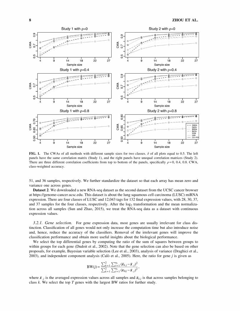
We report the CWAs along with various parameters in Figure 1 for the first two studies, and in Figure 2 for

the last two studies, respectively.

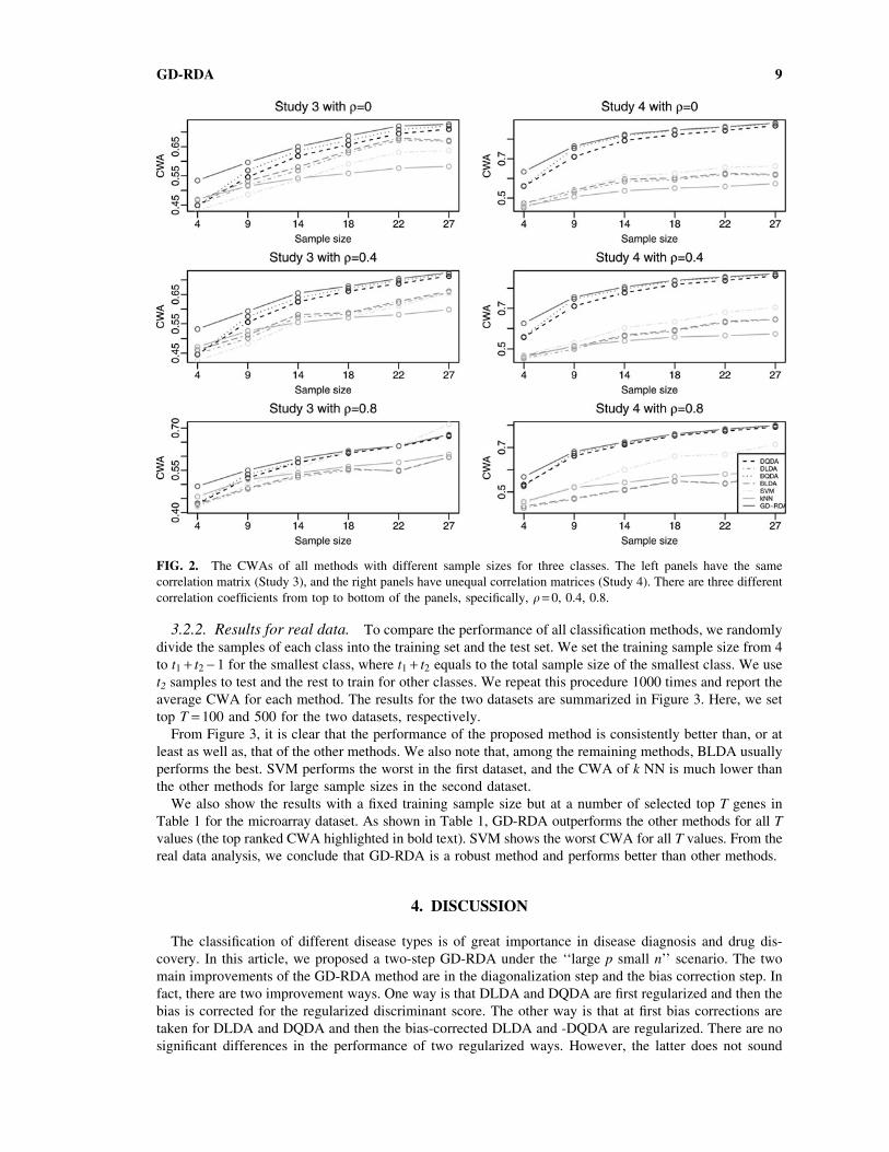
Figures 1 and 2 show that GD-RDA performs significantly better than the other methods in all settings,

especially for small sample sizes. We also note that, among the remaining methods, BQDA usually

performs the best except for the results in Study 1, and SVM and kNN perform the worst in most studies. The

CWAs of all methods increase with increasing the sample size and are related to the different choices of the

correlation coefficient. The CWAs of all methods for q = 0:8 are obviously lower than those for q = 0. In Study

1 (the left panels of Fig. 1), it is evident that BLDA performs a little better than BQDA and is much better than

SVM and k NN. However, in Study 2 (the right panels of Fig. 1), we note that BQDA is much better than

BLDA and is even comparable to GD-RDA when the sample size is large. Relative to Study 2 and Study 4,

the CWAs of GD-RDA are much higher than the second performance method in Study 1 and Study 3.

3.2. Application to real data

We apply the proposed method to two real datasets, including a microarray dataset and an RNA-seq

dataset, and compare it with some existing methods. We first give a brief introduction to the two datasets.

Dataset 1. The microarray dataset is about the breast cancer gene expression, which is available on the

Broad institute http://portals.broadinstitute.org/cgi-bin/cancer/datasets.cgi. As described in Hoshida et al.

(2007), the dataset consists of 1213 genes for 98 final expression values from three classes, including 11,

GD-RDA 7

51, and 36 samples, respectively. We further standardize the dataset so that each array has mean zero and

variance one across genes.

Dataset 2. We downloaded a new RNA-seq dataset as the second dataset from the UCSC cancer browser

at https://genome-cancer.ucsc.edu. This dataset is about the lung squamous cell carcinoma (LUSC) miRNA

expression. There are four classes of LUSC and 12,043 tags for 132 final expression values, with 28, 30, 37,

and 37 samples for the four classes, respectively. After the log2 transformation and the mean normaliza-

tion across all samples (Sun and Zhao, 2015), we treat the RNA-seq data as a dataset with continuous

expression values.

3.2.1. Gene selection. For gene expression data, most genes are usually irrelevant for class dis-

tinction. Classification of all genes would not only increase the computation time but also introduce noise

and, hence, reduce the accuracy of the classifiers. Removal of the irrelevant genes will improve the

classification performance and obtain more useful insights about the biological performance.

We select the top differential genes by computing the ratio of the sum of squares between groups to

within groups for each gene (Dudoit et al., 2002). Note that the gene selection can also be based on other

proposals, for example, Bayesian variable selection (Lee et al., 2003), analysis of variance (Draghici et al.,

2003), and independent component analysis (Calo et al., 2005). Here, the ratio for gene j is given as

BW(j) =P2

k = 1

Pnk

i = 1 (�xk:j - �x::j)2P2

k = 1

Pnk

i = 1 (xkij - �x::j)2

‚

where �x::j is the averaged expression values across all samples and �xk:j is that across samples belonging to

class k. We select the top T genes with the largest BW ratios for further study.

FIG. 1. The CWAs of all methods with different sample sizes for two classes. d of all plots equal to 0.5. The left

panels have the same correlation matrix (Study 1), and the right panels have unequal correlation matrices (Study 2).

There are three different correlation coefficients from top to bottom of the panels, specifically q = 0, 0.4, 0.8. CWA,

class-weighted accuracy.

8 ZHOU ET AL.

3.2.2. Results for real data. To compare the performance of all classification methods, we randomly

divide the samples of each class into the training set and the test set. We set the training sample size from 4

to t1 + t2 - 1 for the smallest class, where t1 + t2 equals to the total sample size of the smallest class. We use

t2 samples to test and the rest to train for other classes. We repeat this procedure 1000 times and report the

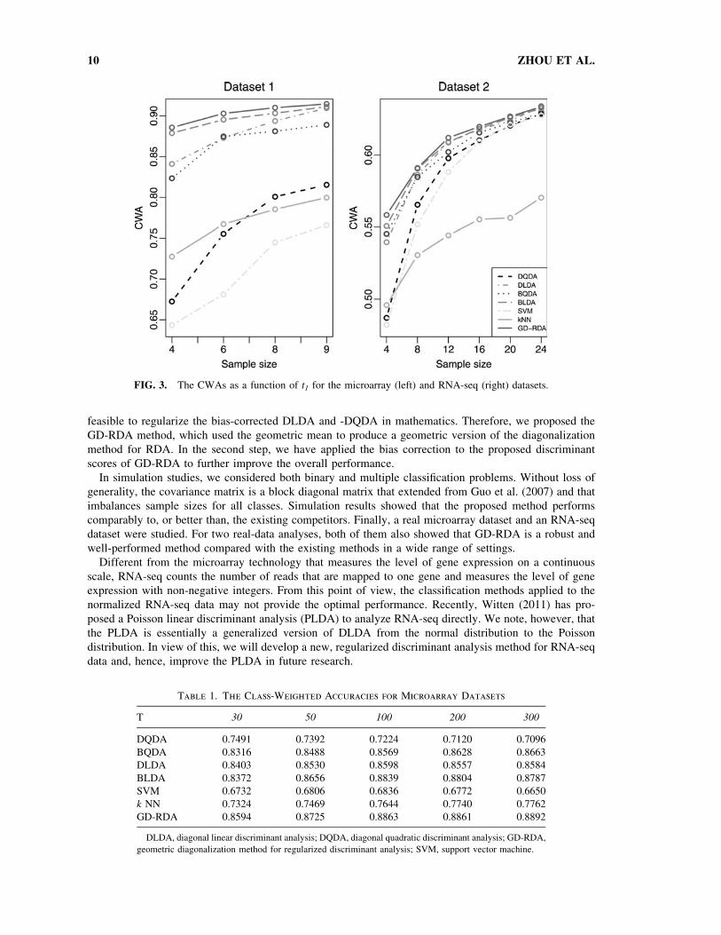
average CWA for each method. The results for the two datasets are summarized in Figure 3. Here, we set

top T = 100 and 500 for the two datasets, respectively.

From Figure 3, it is clear that the performance of the proposed method is consistently better than, or at

least as well as, that of the other methods. We also note that, among the remaining methods, BLDA usually

performs the best. SVM performs the worst in the first dataset, and the CWA of k NN is much lower than

the other methods for large sample sizes in the second dataset.

We also show the results with a fixed training sample size but at a number of selected top T genes in

Table 1 for the microarray dataset. As shown in Table 1, GD-RDA outperforms the other methods for all T

values (the top ranked CWA highlighted in bold text). SVM shows the worst CWA for all T values. From the

real data analysis, we conclude that GD-RDA is a robust method and performs better than other methods.

4. DISCUSSION

The classification of different disease types is of great importance in disease diagnosis and drug dis-

covery. In this article, we proposed a two-step GD-RDA under the ‘‘large p small n’’ scenario. The two

main improvements of the GD-RDA method are in the diagonalization step and the bias correction step. In

fact, there are two improvement ways. One way is that DLDA and DQDA are first regularized and then the

bias is corrected for the regularized discriminant score. The other way is that at first bias corrections are

taken for DLDA and DQDA and then the bias-corrected DLDA and -DQDA are regularized. There are no

significant differences in the performance of two regularized ways. However, the latter does not sound

FIG. 2. The CWAs of all methods with different sample sizes for three classes. The left panels have the same

correlation matrix (Study 3), and the right panels have unequal correlation matrices (Study 4). There are three different

correlation coefficients from top to bottom of the panels, specifically, q = 0, 0.4, 0.8.

GD-RDA 9

feasible to regularize the bias-corrected DLDA and -DQDA in mathematics. Therefore, we proposed the

GD-RDA method, which used the geometric mean to produce a geometric version of the diagonalization

method for RDA. In the second step, we have applied the bias correction to the proposed discriminant

scores of GD-RDA to further improve the overall performance.

In simulation studies, we considered both binary and multiple classification problems. Without loss of

generality, the covariance matrix is a block diagonal matrix that extended from Guo et al. (2007) and that

imbalances sample sizes for all classes. Simulation results showed that the proposed method performs

comparably to, or better than, the existing competitors. Finally, a real microarray dataset and an RNA-seq

dataset were studied. For two real-data analyses, both of them also showed that GD-RDA is a robust and

well-performed method compared with the existing methods in a wide range of settings.

Different from the microarray technology that measures the level of gene expression on a continuous

scale, RNA-seq counts the number of reads that are mapped to one gene and measures the level of gene

expression with non-negative integers. From this point of view, the classification methods applied to the

normalized RNA-seq data may not provide the optimal performance. Recently, Witten (2011) has pro-

posed a Poisson linear discriminant analysis (PLDA) to analyze RNA-seq directly. We note, however, that

the PLDA is essentially a generalized version of DLDA from the normal distribution to the Poisson

distribution. In view of this, we will develop a new, regularized discriminant analysis method for RNA-seq

data and, hence, improve the PLDA in future research.

Table 1. The Class-Weighted Accuracies for Microarray Datasets

T 30 50 100 200 300

DQDA 0.7491 0.7392 0.7224 0.7120 0.7096

BQDA 0.8316 0.8488 0.8569 0.8628 0.8663

DLDA 0.8403 0.8530 0.8598 0.8557 0.8584

BLDA 0.8372 0.8656 0.8839 0.8804 0.8787

SVM 0.6732 0.6806 0.6836 0.6772 0.6650

k NN 0.7324 0.7469 0.7644 0.7740 0.7762

GD-RDA 0.8594 0.8725 0.8863 0.8861 0.8892

DLDA, diagonal linear discriminant analysis; DQDA, diagonal quadratic discriminant analysis; GD-RDA,

geometric diagonalization method for regularized discriminant analysis; SVM, support vector machine.

FIG. 3. The CWAs as a function of t1 for the microarray (left) and RNA-seq (right) datasets.

10 ZHOU ET AL.

5. APPENDIX

Proof of Theorem 1

To correct the bias for the discriminant score ~dRk (y) (2.11), the plug-in estimates ~Lk1 and ~Lk2 are used for

estimating Lk1 and Lk2, respectively. In what follows, we show that both ~Lk1 and ~Lk2 are biased estimators

for any fixed k. We then purpose two unbiased estimators for these two quantities and use them to form a

bias-corrected rule for regularized discriminant analysis.

By (2.1), we have �xki*N(lki‚ r2ki=nk) and s2

ki*r2kiv

2nk - 1=(nk - 1) for any i = 1‚ . . . ‚ p and k = 1‚ . . . ‚ K, where

v2� is the chi-square distribution with � degrees of freedom. Then, by s2

pool‚ i =QK

k = 1 s2ki

� �1=Kand the fact that

s21i‚ . . . ‚ s2

ki and �xki are mutually independent, for the plug-in estimator ~Lk1 we have

E(~Lk1) =Xp

i = 1

E(yi - �xki)2E (s2

ki)k - 1

(s2pool‚ i)

- kh i

=Xp

i = 1

E(yi - �xki)2E(s2

1i)- k

K � � �

E(s2ki)

k - 1 - kK � � �E(s2

Ki)- k

K

=Xp

i = 1

(yi - lki)2 +

r2ki

nk

� �(r2

1i)- k

K

h(n1‚ - kK

)

� � � (r2ki)

k - 1 - kK

h(nk‚ k - 1 - kK

)� � � (r2

Ki)- k

K

h(nK‚ - kK

)

=1

Bk

Xp

i = 1

(yi - lki)2 +

r2ki

nk

� �(r2

ki)k - 1(r2

pool‚ i)- k

=1

Bk

Lk1 +pCk

nkBk

‚

(5:13)

where Bk = (h(nk‚ k - 1 - kK

)=h(nk‚ - kK

))QK

j = 1 h(nj‚ - kK

) and

Ck =1

p

Xp

i = 1

r2ki

r2pool‚ i

!k

:

Note that Ck is unknown in practice since it involves the unknown variances. We propose to estimate Ck by

Ck =Dk

p

Xp

i = 1

s2ki

s2pool‚ i

!k

‚ (5:14)

where Dk = h(nk‚ k - kK

)h(nk‚ kK

)=QK

j = 1 h(nj‚kK

). To investigate the asymptotic properties of Ck‚ we consider

the ratios r2ki=r

2pool‚ i as a random sample of size p from a common distribution F with a finite second

moment. Then, by the strong law of large numbers, it is easy to verify that Ck - Ck!a:s:

0 as p!1, where!a:s:

represents almost sure convergence. Finally, by (5.13) and (5.14), we propose the following asymptotically

unbiased estimator for Lk1:

L^

k1 = Bk

Xp

i = 1

(yi - �xki)2

(s2ki)

1 - k(s2

pool‚ i)k

-Dk

nk

Xp

i = 1

s2ki

s2pool‚ i

!k

: (5:15)

Now for the plug-in estimator ~Lk2, to calculate its expectation, we need to apply the formula that

E( ln v2�) =C(�=2) + ln 2, where C(�) is the so-called digamma function proposed by Abramowitz and

Stegun (1972). Then by the facts that s2pool‚ i =

QKk = 1 s2

ki

� �1=Kand s2

ki*r2kiv

2nk - 1=(nk - 1), we have

GD-RDA 11

E(~Lk2) = (1 - k)Xp

i = 1

E( ln s2ki) +

kK

Xp

i = 1

XK

j = 1

E( ln s2ji)

= (1 - k)Xp

i = 1

C(nk - 1

2) + ln 2 + ln

r2ki

nk - 1

� �� �

+kK

Xp

i = 1

XK

j = 1

C(nj - 1

2) + ln 2 + ln

r2ji

nj - 1

!" #

= Lk2 + Ek‚

(5:16)

where Ek = (1 - k)p(C(nk - 12

) - ln (nk - 12

)) + kpK

PKj = 1 (C(

nj - 1

2) - ln (

nj - 1

2)). By (5.16), we propose the following

unbiased estimator for Lk2:

�Lk2 =Xp

i = 1

ln (s2ki)

1 - k(s2

pool‚ i)k

h i- Ek: (5:17)

Finally, by the proposed bias-corrected estimators (5.15) and (5.17), we get the bias-corrected discriminant

score as follows:

�dRk (y) = �Lk1 + �Lk2 - 2 ln pk‚

This completes the proof of the theorem.

ACKNOWLEDGMENTS

The authors thank the editor, the associate editor, and the referees for their constructive comments that

led to a substantial improvement of the paper. Xiang Wan’s research was supported by Hong Kong RGC

grant HKBU12202114 and the National Natural Science Foundation of China (Grant No. 61501389).

Tiejun Tong’s research was supported by the Hong Kong Baptist University grants FRG1/14-15/084,

FRG2/15-16/019 and FRG2/15-16/038, and the National Natural Science Foundation of China (Grant No.

11671338). Yan Zhou’s research was supported by Tianyuan fund for Mathematics (Grant No. 11526143),

Doctor start fund of Guangdong Province [No. 2016A030310062 (85118-000043)], and The Natural

Science Foundation of SZU (Grant No. 836-00008303). Gaorong Li’s research was supported by the

National Natural Science Foundation of China (Grant No. 11471029), the Beijing Natural Science Foun-

dation (Grant No. 1142002), and the Science and Technology Project of Beijing Municipal Education

Commission (Grant No. KM201410005010). Baoxue Zhang’s research was supported by the National

Science Foundation of China (Grant No. 11671268). The ‘‘GDRDA’’ package is made in the form of an R

code, and the complete documentation is available on request from the corresponding author.

AUTHOR DISCLOSURE STATEMENT

No competing financial interests exist.

REFERENCES

Abramowitz, M., and Stegun, I.A. 1972. Handbook of Mathematical Functions. Dover, New York.

Bickel, P.J., and Levina, E. 2004. Some theory of Fisher’s linear discriminant function, naive Bayes, and some

alternatives when there are many more variables than observations. Bernoulli. 10, 989–1010.

Calo, D.G., Galimberti, G., Pillati, M., et al. 2005. Variable selection in classification problems: A strategy based on

independent component analysis, 21–30. In Vichi, M. et al., eds. New Developments in Classification and Data

Analysis. Studies in Classification, Data Analysis, and Knowledge Organization. Springer, Berlin.

Cohen, G., Hilario, M., Sax, H., et al. 2006. Learning from imbalanced data in surveillance of nosocomial infection.

Artif. Intell. Med. 37, 7–18.

12 ZHOU ET AL.

Draghici, S., Olga, K., Hoff, B., et al. 2003. Noise sampling method: An ANOVA approach allowing robust selection of

differentially regulated genes measured by DNA microarrays. Bioinformatics. 19, 1348–1359.

Dudoit, S., Fridlyand, J., and Speed, T.P. 2002. Comparison of discrimination methods for the classification of tumors

using gene expression data. J. Am. Stat. Assoc. 97, 77–87.

Friedman, J.H. 1989. Regularized discriminant analysis. J. Am. Stat. Assoc. 84, 165–175.

Guo, Y., Hastie, T., and Tibshirani, R. (007. Regularized linear discriminant analysis and its application in microarrays.

Biostatistics. 8, 86–100.

Hoshida, Y.J., Brunet, J.P., Tamayo, P., et al. 2007. Subclass mapping: Identifying common subtypes in independent

disease data sets. PLoS One. 2, e1195.

Huang, S., Tong, T., and Zhao, H. 2010. Bias-corrected diagonal discriminant rules for high-dimensional classification.

Biometrics. 66, 1096–1106.

James, W., and Stein, C. 1961. Estimation with quadratic loss, 361–379. In Proceedings of the Fourth Berkeley

Symposium on Mathematical Statistics and Probability, Vol. 1. Publisher: University of California, Berkley.

Kaur, S., Archer, K.J., Devi, M.G., et al. 2012. Differential gene expression in granulosa cells from polycystic ovary

syndrome patients with and without insulin resistance: Identification of susceptibility gene sets through network

analysis. J. Clin. Endocrinol. Metab. 97, E2016–E2021.

Lee, J.W., Lee, J.B., Park, M., et al. 2005. An extensive comparison of recent classification tools applied to microarray

data. Comput. Stat. Data Anal. 48, 869–885.

Lee, K.E., Sha, N.J., Dougherty, E.R., et al. 2003. Gene selection: A Bayesian variable selection approach. Bioin-

formatics. 19, 90–97.

Mardis, E.R. 2008. Next-generation DNA sequencing methods. Annu. Rev. Genomics Hum. Genet. 9, 387–402.

McLachlan, G.J. 1992. Discriminant Analysis and Statistical Pattern Recognition. Wiley, New York.

Mokry, M., Hatzis, P., Schuijers, J., et al. 2012. Integrated genome-wide analysis of transcription factor occupancy,

RNA polymerase II binding and steady-state RNA levels identify differentially regulated functional gene classes.

Nucleic Acids Res. 40, 148–158.

Moran, M.A., and Murphy, B.J. 1979. A closer look at two alternative methods of statistical discrimination. Appl. Stat.

28, 223–232.

Morozova, O., Hirst, M., and Marra, M.A. 2009. Applications of new sequencing technologies for transcriptome

analysis. Annu. Rev. Genomics Hum. Genet. 10, 135–151.

Pang, H., Tong, T., and Zhao, H. 2009. Shrinkage-based diagonal discriminant analysis and its applications in high-

dimensional data. Biometrics. 65, 1021–1029.

Qiao, X., and Liu, Y. 2009. Adaptive weighted learning for unbalanced multicategory classification. Biometrics. 65,

159–168.

Radchenko, R., and James, G.M. 2008. Variable inclusion and shrinkage algorithms. J. Am. Stat. Assoc. 103, 1304–

1315.

Ripley, B.D. 1996. Pattern Recognition and Neural Networks. Cambridge, Cambridge University Press.

Searcy, J.L., Phelps, J.T., Pancani, T., et al. 2012. Long-term pioglitazone treatment improves learning and attenuates

pathological markers in a mouse model of Alzheimer’s disease. J. Alzheimers Dis. 30, 943–961.

Sun, J.H., and Zhao, H. 2015. The application of sparse estimation of covariance matrix to quadratic discriminant

analysis. BMC Bioinformatics. 16, 48.

Tong, T., and Wang, Y. 2007. Optimal shrinkage estimation of variances with applications to microarray data analysis.

J. Am. Stat. Assoc. 102, 113–122.

Wang, Z., Gerstein, M., and Snyder, M. 2009. RNA-Seq: A revolutionary tool for transcriptomics. Nat. Rev. Genet. 10,

57–63.

Address correspondence to:

Dr. Xiang Wan

Department of Computer Science

Hong Kong Baptist University

Kowloon Tong

Hong Kong, China

E-mail: xwan@comp.hkbu.edu.hk

GD-RDA 13