Joint Effects of Extrinsic Biophysical Fluxes and IntrinsicHydrodynamics on the Formation of HypoxiaWest off the Pearl River EstuaryZhongming Lu1,2 , Jianping Gan3,4,5 , Minhan Dai6 , Hongbin Liu3,5,7, and Xiaozheng Zhao1

1Division of Environment and Sustainability, Hong Kong University of Science and Technology, Hong Kong, 2Institute forAdvanced Study, Hong Kong University of Science and Technology, Hong Kong, 3Department of Ocean Science,Hong Kong University of Science and Technology, Hong Kong, 4Department of Mathematics, Hong Kong University ofScience and Technology, Hong Kong, 5State Key Laboratory in Marine Pollution, Hong Kong, 6State Key Laboratory ofMarine Environment, Xiamen University, Xiamen, China, 7Division of Life Science, Hong Kong University of Science andTechnology, Hong Kong

Abstract Using fieldmeasurements and a process-oriented three-dimensional coupled physical-biogeochemicalnumerical model, we investigated the physical and biogeochemical processes governing the bottom hypoxiczone west off the Pearl River estuary. The intensity and area of the hypoxia grew with increasing totalnutrient input from the Pearl River that has increased continuously in recent decades. The hypoxic zone wasformed and maintained largely associated with the stable water column where the stability was providedsimultaneously by wind stress and freshwater discharge, favorable local hydrodynamics for flow convergence,and westward organic matter transport. Wind stress altered the stratification, while freshwater dischargechanged the stratification and baroclinic velocity shear simultaneously. Two-layered flow with a cyclonicallyrotating current around a coastal salient edge of the western shelf off the estuary hydrodynamically enhancedthe local convergence, allowing sufficient residence time in the bottom for the remineralization of organicmatter produced in the hypoxic zone and organic matter transported into the region. Our results suggestthat a combination of unique local hydrodynamic feature and decomposition of organic matter in watercolumn (and possibly in the sediment) are the cause of the formation andmaintenance of the bottom hypoxiaon the western shelf of the estuary during summer.

Plain Language Summary Hypoxia results in dead zones in the ocean. It often occurs in the bottomwaters below surface eutrophication due to decomposition of organic matter in the water column andalso possibly in sediment. Both physical and biogeochemical processes in the ocean control the formation ofthe eutrophication and hypoxia. This study investigates these processes for an observed strong hypoxia zoneoff Pearl River estuary using a numerical model and field measurement data. Through comprehensiveanalyses, we found that the intensity and area of the hypoxia grew with increasing total nutrient input fromPearl River. The hydrodynamic conditions of ocean flow field such as stability of the water column associatedwith wind forcing and freshwater buoyancy discharge, local flow convergence, and external organicmatter input provide favorable conditions for the formation of hypoxia.

1. Introduction

Hypoxia occurs when oxygen consumption in the water column cannot be replenished by supply. When thelevel of dissolved oxygen (DO) falls below 2–3mg/L, hypoxia appears (Chu et al., 2005; Dai et al., 2006; Rabalaiset al., 2002). Both natural processes and anthropogenic activities can lead to hypoxia in a marine environment.Hypoxia occurs naturally in upwelling zones with high productivity or in restricted basins and fjords wherewater exchanges are limited (Helly & Levin, 2004; Rabalais et al., 2010; F. Zhang, 2001). Hypoxia due to anthro-pogenic activities is a consequence of eutrophication driven by the increasing human input of nutrients andorganic matter (Cai et al., 2011). Hypoxia has been spreading rapidly in frequency and extent in coastal andestuarine areas, which has important environmental consequence (Breitburg et al., 2018).

Many studies indicate that the remineralization of organic matter in the hypoxic zone is associated with auto-chthonous organic carbon production fueled by excessive terrestrial nutrient input (Rabalais et al., 2014;Turner & Rabalais, 1994; H. J. Wang et al., 2016; J. Zhang et al., 2010). Hypoxia generally has a positive

LU ET AL. 1

Journal of Geophysical Research: Oceans

RESEARCH ARTICLE10.1029/2018JC014199

Key Points:• The hypoxia west off Pearl River

estuary is extrinsically controlled bybiophysical fluxes and intrinsically bylocal hydrodynamics

• Remineralization of organic matter inthe water column and sediment andlocal unique hydrodynamics formedand maintained the bottom hypoxia

• Water column stability was providedby wind and freshwater dischargewhile local rotating current providedfavorable residence time

Supporting Information:• Supporting Information S1• Data Set S1

Correspondence to:J. Gan,magan@ust.hk

Citation:Lu, Z., Gan, J., Dai, M., Liu, H., & Zhao, X.(2018). Joint effects of extrinsicbiophysical fluxes and intrinsichydrodynamics on the formation ofhypoxia west off the Pearl River estuary.Journal of Geophysical Research: Oceans,123. https://doi.org/10.1029/2018JC014199

Received 22 MAY 2018Accepted 26 JUL 2018Accepted article online 8 AUG 2018

©2018. American Geophysical Union.All Rights Reserved.

correlation with nutrient loading (Hagy et al., 2004). Other studies suggest that oxygen is consumed in thewater column through the aerobic respiration of allochthonous organic matter coming from wastewaterdischarge and nitrification (Dagg et al., 2007; He et al., 2014; Swarzenski et al., 2008). In addition to thebiogeochemical controls in generating hypoxic zones, hydrodynamics plays a critically important role. Forexample, stratification can inhibit ventilation and reduce oxygen replenishment in the bottom layer.Stratification can be regulated by freshwater discharge from large rivers (Bianchi et al., 2010; Wisemanet al., 1997) due to the buoyancy flux. Local wind forcing also affects vertical circulation and mixing (L. X.Wang & Justic, 2009).

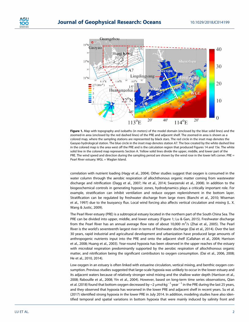
The Pearl River estuary (PRE) is a subtropical estuary located in the northern part of the South China Sea. ThePRE can be divided into upper, middle, and lower estuary (Figure 1; Lu & Gan, 2015). Freshwater dischargefrom the Pearl River has an annual average flow rate of about 10,000 m3/s (Zhai et al., 2005). The PearlRiver is the world’s seventeenth largest river in terms of freshwater discharge (Dai et al., 2014). Over the last30 years, rapid industrial and agricultural development and urbanization have produced large amounts ofanthropogenic nutrients input into the PRE and onto the adjacent shelf (Callahan et al., 2004; Harrisonet al., 2008; Huang et al., 2003). Year-round hypoxia has been observed in the upper reaches of the estuarywith microbial respiration predominantly supported by the aerobic respiration of allochthonous organicmatter, and nitrification being the significant contributors to oxygen consumption. (Dai et al., 2006, 2008;He et al., 2010, 2014).

Low oxygen in an estuary is often linked with estuarine circulation, vertical mixing, and benthic oxygen con-sumption. Previous studies suggested that large-scale hypoxia was unlikely to occur in the lower estuary andits adjacent waters because of relatively stronger wind mixing and the shallow water depth (Harrison et al.,2008; Rabouille et al., 2008; Yin et al., 2004). However, based on long-term time series observations, Qianet al. (2018) found that bottom oxygen decreased by ~2 μmol·kg�1·year�1 in the PRE during the last 25 years,and they observed that hypoxia has worsened in the lower PRE and adjacent shelf in recent years. Su et al.(2017) identified strong hypoxia in the lower PRE in July 2014. In addition, modeling studies have also iden-tified temporal and spatial variations in bottom hypoxia that were mainly induced by salinity front and

Figure 1. Map with topography and isobaths (in meters) of the model domain (enclosed by the blue solid lines) and thezoomed-in area (enclosed by the red dashed lines) of the PRE and adjacent shelf. The zoomed-in area is shown as acolored map, where the sampling stations are represented by black stars. The red circle in the inset map denotes theGaoyao hydrological station. The blue circle in the inset map denotes station A7. The box created by the white dashed linein the colored map is the area west off the PRE and is the calculation region that produced Figures 14 and 15e. The whitesolid line in the colored map represents Section A. Yellow solid lines divide the upper, middle, and lower part of thePRE. The wind speed and direction during the sampling period are shown by the wind rose in the lower left corner. PRE =Pearl River estuary; WGL = Waglan Island.

10.1029/2018JC014199Journal of Geophysical Research: Oceans

LU ET AL. 2

stratification (Luo et al., 2009). H. Zhang and Li (2010) investigated the sources and sinks of oxygen in the PREand found that sediment oxygen demand played the dominant role in hypoxia generation because of theshallow topography and high deposition rate of particulate organic matters. Wei et al. (2016) explored theeffects of wind and river discharge on hypoxia on the eastern side of the lower PRE during summer. They indi-cated that the hypoxic zone responded differently to changes of river discharge at different inlets and thatthe wind speed had a stronger effect on hypoxia than the wind direction. B. Wang et al. (2017) investigatedthe oxygen dynamics in the PRE and found that re-aeration and sediment oxygen demands were the twomajor processes controlling the bottom hypoxia in this region.

Despite themany observational andmodeling efforts, there remain numerous uncertainties on the formationprocess of hypoxia or the role of spatiotemporally varying coupled physical-biogeochemical processes onhypoxia generation in the PRE. Furthermore, hypoxia studies in the PRE have mainly focused on axial transectof PRE and the eastern side of the lower PRE when Pearl River plume was advected eastward by the south-westerly wind-driven coastal current during summer (Gan, Li, et al., 2009). Few studies have investigatedhypoxia occurring west off the PRE. We know little about hypoxia on the western side of the PRE and adjacentcoastal waters so far. Furthermore, nutrient loading in the PRE increased more than sevenfold during the lastthree decades (Ma et al., 2009), and a much stronger hypoxia as compared to those observed in the previousstudies can be expected nowadays.

In this study, we investigated the time-dependent, three-dimensional evolution of hypoxia on the westernshelf off the PRE under various control factors by elucidating the biogeochemical processes. We usedprocess-oriented numerical experiments to reveal the fundamental processes that controlled the intensityand location of bottom hypoxia in the region.

2. Materials and Methods2.1. Observational Data

We used field measurements from 5 to 17 July 2015. The measurements helped identify the characteristics ofhypoxia on the western shelf off the PRE and informed themodeling study. The field survey occurred during atypical summer southwesterly monsoon (Figure 1).

We measured salinity and temperature using a Seabird 911 plus conductivity-temperature-depth profiler(Sea Bird Electronics, Inc.) with a precision of ±0.0005 S/m and ± 0.005 °C. The conductivity-tempera-ture-depth was raised and lowered at ~0.2 m/s. We collected the discrete samples of nitrate (NO3) andphosphate (PO4) using a Rosette sampler with GO-FLO bottles (General Oceanics Co.). We determinedNO3 and PO4 colorimetrically using a flow injection analyzer (QuAAtro nutrient analyzer, Seal Analytical,Inc.) with the detection limits of 0.04 and 0.08 μM, respectively. We determined chlorophyll-a using thestandard fluorometric method (Parsons et al., 1984) and a Trilogy laboratory fluorometer (TurnerDesigns, Inc.) with a detection limit of 0.025 μg/L. We measured DO using the Winkler titration method(Bryan et al., 1976) with a precision of ±0.06 mg/L. We obtained long-term wind speed at Waglan Island(WGL) and river discharge data at Gaoyao station from the Hong Kong Observatory (http://www.weather.gov.hk/wxinfo/ts/display_element_ff_e.htm) and the Information Center of Water Resources, Bureau ofHydrology, the Ministry of Water Resources of P. R. China (http://xxfb.hydroinfo.gov.cn/ssIndex.html),respectively. The wind speed and discharge served as references for setting up the sensitivity cases inour numerical study.

2.2. Ocean Model and Implementation

We developed a coupled physical-biological model for the PRE based on a validated physical model by Zuand Gan (2015). The physical model adopts the hydrostatic primitive Regional Ocean Modeling System(ROMS; Shchepetkin & McWilliams, 2005). Our computational domain extends from 20.9°N, 112.7°E in thesouthwest corner to 23.3°N, 115.0°E in the northeast corner (Figure 1). The curvilinear grid with a (400,200)-dimensional array for the horizontal coordinates (x, y) has a horizontal resolution of ~0.8 km.Vertically, we adopted a 30-level stretched generalized terrain-following coordinate system with higherresolution in the surface and bottom layers. Other relevant details about the numerical techniques and imple-mentations can be found in Zu and Gan (2015).

10.1029/2018JC014199Journal of Geophysical Research: Oceans

LU ET AL. 3

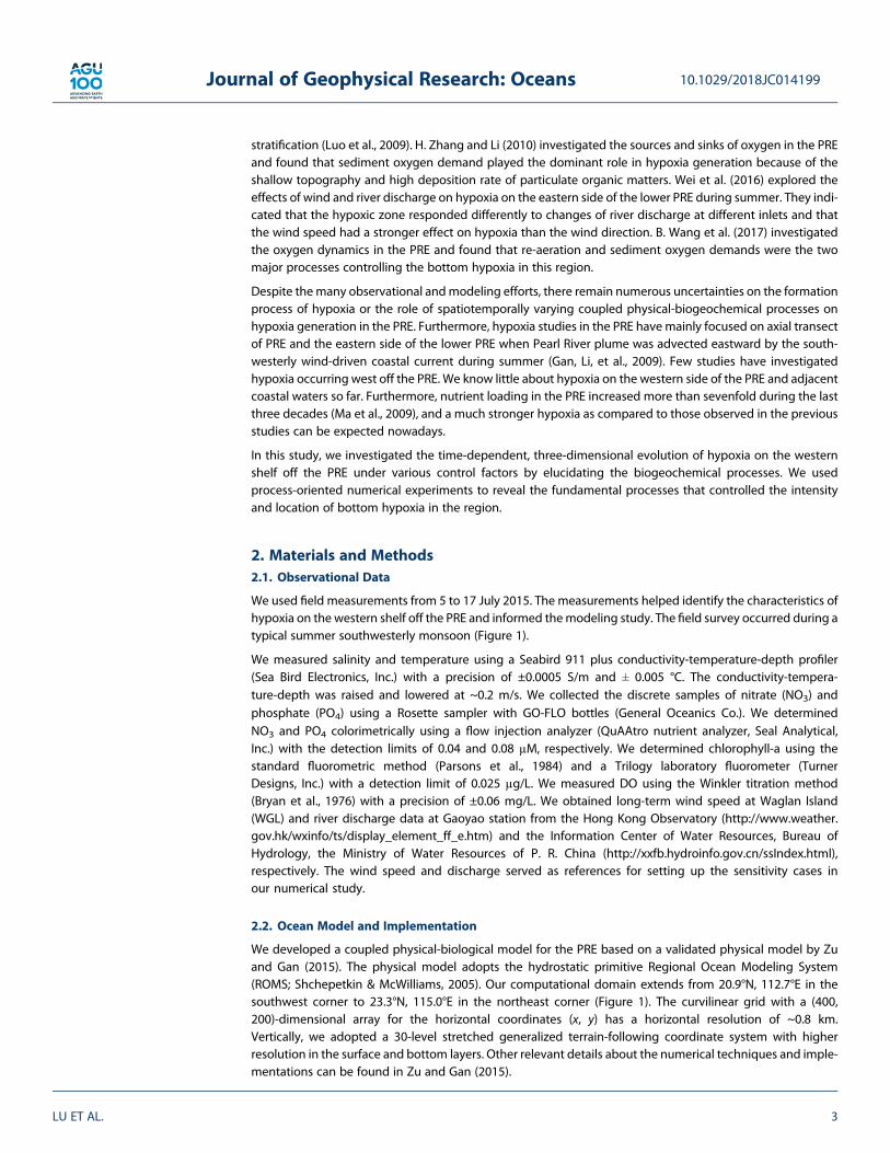
The biological model was coupled with the physical model at identical temporal and spatial resolutions. It is anitrogen, phosphorus, phytoplankton, zooplankton, and detritus (NPPZD) model (Figure 2) that Gan et al.(2014) developed. The model is based on the ROMS biological module to reflect the P limitation status thatwidely exists in estuarine and coastal waters (Gan et al., 2014). The biological parameters (Table 1) adopted inthe NPPZD model were set based on previous studies in this region and on studies of other oceans aroundthe world (Fennel et al., 2006; Gan et al., 2014; Spitz et al., 2005). We adopted the oxygen model of Fennelet al. (2006), in which oxygen was consumed by remmineralization of organic matter, biological matabolism,and nitritification of ammonium to nitrate in both water column and sediment (Figure 2 and equation (A4) inAppendix A).

We conducted a process-oriented modeling study by forcing the model with a typical southwesterly windstress equal to 0.025 Pa (Gan, Cheung, et al., 2009) over the entire computational domain. The underlying pro-cessesandmechanismsofhypoxiadevelopment involvemultiforcing in thecomplexcoupledphysical andbio-geochemical system.We adopt process-orientedmodeling based on the simplified but representative forcingin order to better isolate the processes, which otherwise may not be able to resolve solidly (Zu & Gan, 2015).

We initialized the model with horizontally uniform salinity, temperature, NO3, PO4, DO, and chlorophyllprofiles obtained from the field measurements at Station A7 (Figure 1). We calculated the initial values ofphytoplankton, zooplankton, and detritus from chlorophyll data by assuming the ratios of 1.59, 0.3, and 0.7for chlorophyll/phytoplankton, zooplankton/phytoplankton, and detritus/phytoplankton, respectively (Ganet al., 2014).

To investigate the impact of external forcing, we applied an active open boundary condition (OBC; Gan &Allen, 2005) to the open boundaries of our computational domain (Figure 1). The active OBC is able to inte-grate the effect of external forcing along the open boundaries into the simulation. In our case, the summer(June to August) mean variables obtained from a model that covered the entire northern South China Seashelf (Gan, Li, et al., 2009; Gan et al., 2014) provided the external physical and biogeochemical fluxes. Inour sensitivity experiments, in order to investigate the impacts of local forcing (e.g., river discharge and wind)on hypoxia, we excluded the effects from external biogeochemical forcing by applying a passive OBC for allbiogeochemical variables.

Figure 2. Schematic of the biogeochemical model. The boxes represent the biogeochemical variables. The boxes aboveand below the gray dashed line represent variables in the water column and sediment, respectively. The black arrowsindicate the biogeochemical processes of the aquatic ecosystem. The green arrows represent the processes in the sedi-ment. The dashed arrows represent the air-sea oxygen exchange.

10.1029/2018JC014199Journal of Geophysical Research: Oceans

LU ET AL. 4

We set the river discharge to 18,400 m3/s and the daily average solar radiation to 195 W/m2 with a diurnalcycle distribution. We made the salinity, temperature, NO3, and PO4 of the river water equal to 3 practicalsalinity units, 28.6 °C, 60 μM, and 1 μM (Cai et al., 2004), respectively. We neglected contribution of riverineinput of organic matter to the hypoxia, because most of the phytoplankton from the river discharge are inac-tive (Dai et al., 2008; Lu & Gan, 2015), and most of the oxygen-consuming organic matter were derived frommarine sources (Qian et al., 2018; Su et al., 2017). The model was run for 50 days.

3. Observational Features and Model Results

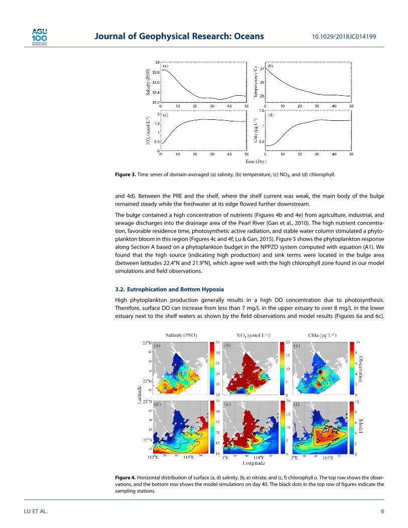
The field observations and model simulations illustrate the biogeochemical features of the PRE and the adja-cent shelf for typical summer conditions. Figure 3 shows the time series of model-simulated domain-averaged salinity, temperature, NO3, and chlorophyll. The model was run for 50 days, and it reached the phy-sical and biogeochemical quasi steady state in about 30 days. We analyzed the quasi-steady model outputson day 40.

3.1. River Plume and Ecosystem Responses

Figure 4 shows the observed and simulated horizontal distributions of surface salinity, NO3, and chlorophyll(Chl-a). The observed and the modeled distributions exhibit qualitatively similar biophysical features.Phytoplankton biomass began to appear in the middle of the estuary several days after the freshwater input,thenmoved downstream as freshwater gradually filled the whole estuary. It reached equilibrium at about day20. In the upper andmiddle estuaries, phytoplankton levels remained very low although the nutrient concen-tration was high, likely due to the strong flushing of river discharge and high water turbidity (Lu & Gan, 2015).The freshwater veered westward inside the PRE but advected eastward over the shelf because of the upwel-ling shelf current (Gan, Li, et al., 2009). When the freshwater input from the Pearl River exited themouth of thePRE, a southeastward-expanding freshwater bulge formed outside the entrance of the estuary (Figures 4a

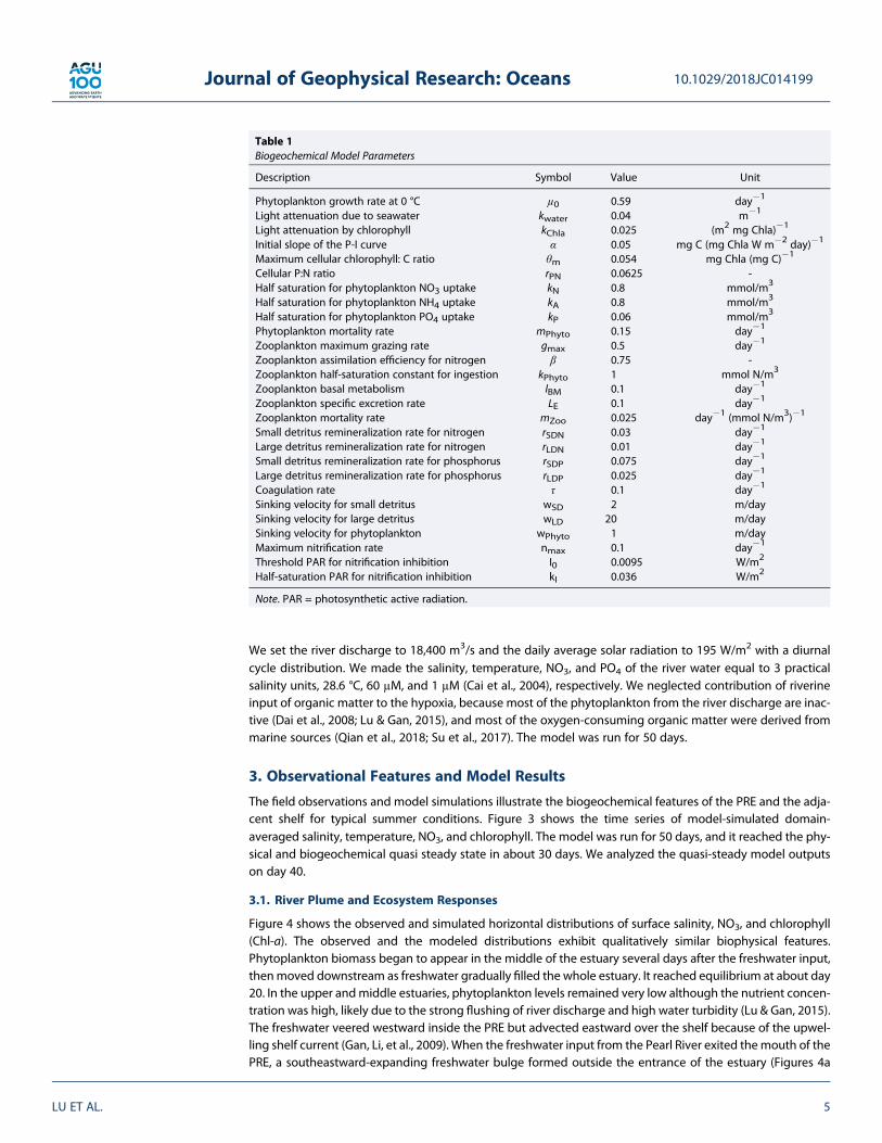
Table 1Biogeochemical Model Parameters

Description Symbol Value Unit

Phytoplankton growth rate at 0 °C μ0 0.59 day�1

Light attenuation due to seawater kwater 0.04 m�1

Light attenuation by chlorophyll kChla 0.025 (m2 mg Chla)�1

Initial slope of the P-I curve α 0.05 mg C (mg Chla W m�2 day)�1

Maximum cellular chlorophyll: C ratio θm 0.054 mg Chla (mg C)�1

Cellular P:N ratio rPN 0.0625 -Half saturation for phytoplankton NO3 uptake kN 0.8 mmol/m3

Half saturation for phytoplankton NH4 uptake kA 0.8 mmol/m3

Half saturation for phytoplankton PO4 uptake kP 0.06 mmol/m3

Phytoplankton mortality rate mPhyto 0.15 day�1

Zooplankton maximum grazing rate gmax 0.5 day�1

Zooplankton assimilation efficiency for nitrogen β 0.75 -Zooplankton half-saturation constant for ingestion kPhyto 1 mmol N/m3

Zooplankton basal metabolism lBM 0.1 day�1

Zooplankton specific excretion rate LE 0.1 day�1

Zooplankton mortality rate mZoo 0.025 day�1 (mmol N/m3)�1

Small detritus remineralization rate for nitrogen rSDN 0.03 day�1

Large detritus remineralization rate for nitrogen rLDN 0.01 day�1

Small detritus remineralization rate for phosphorus rSDP 0.075 day�1

Large detritus remineralization rate for phosphorus rLDP 0.025 day�1

Coagulation rate τ 0.1 day�1

Sinking velocity for small detritus wSD 2 m/daySinking velocity for large detritus wLD 20 m/daySinking velocity for phytoplankton wPhyto 1 m/dayMaximum nitrification rate nmax 0.1 day�1

Threshold PAR for nitrification inhibition I0 0.0095 W/m2

Half-saturation PAR for nitrification inhibition kI 0.036 W/m2

Note. PAR = photosynthetic active radiation.

10.1029/2018JC014199Journal of Geophysical Research: Oceans

LU ET AL. 5

and 4d). Between the PRE and the shelf, where the shelf current was weak, the main body of the bulgeremained steady while the freshwater at its edge flowed further downstream.

The bulge contained a high concentration of nutrients (Figures 4b and 4e) from agriculture, industrial, andsewage discharges into the drainage area of the Pearl River (Gan et al., 2010). The high nutrient concentra-tion, favorable residence time, photosynthetic active radiation, and stable water column stimulated a phyto-plankton bloom in this region (Figures 4c and 4f; Lu & Gan, 2015). Figure 5 shows the phytoplankton responsealong Section A based on a phytoplankton budget in the NPPZD system computed with equation (A1). Wefound that the high source (indicating high production) and sink terms were located in the bulge area(between latitudes 22.4°N and 21.9°N), which agree well with the high chlorophyll zone found in our modelsimulations and field observations.

3.2. Eutrophication and Bottom Hypoxia

High phytoplankton production generally results in a high DO concentration due to photosynthesis.Therefore, surface DO can increase from less than 7 mg/L in the upper estuary to over 8 mg/L in the lowerestuary next to the shelf waters as shown by the field observations and model results (Figures 6a and 6c).

Figure 3. Time series of domain-averaged (a) salinity, (b) temperature, (c) NO3, and (d) chlorophyll.

Figure 4. Horizontal distribution of surface (a, d) salinity, (b, e) nitrate, and (c, f) chlorophyll a. The top row shows the obser-vations, and the bottom row shows the model simulations on day 40. The black dots in the top row of figures indicate thesampling stations.

10.1029/2018JC014199Journal of Geophysical Research: Oceans

LU ET AL. 6

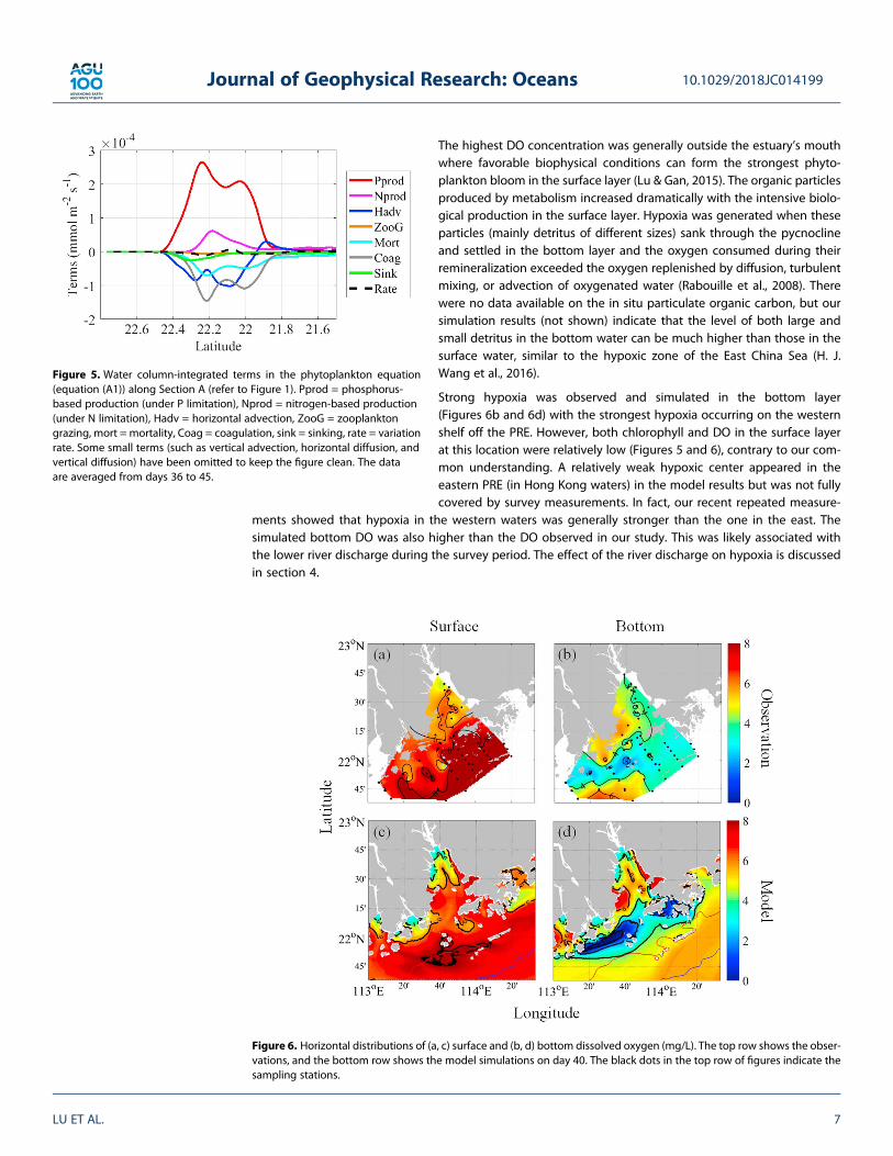
The highest DO concentration was generally outside the estuary’s mouthwhere favorable biophysical conditions can form the strongest phyto-plankton bloom in the surface layer (Lu & Gan, 2015). The organic particlesproduced by metabolism increased dramatically with the intensive biolo-gical production in the surface layer. Hypoxia was generated when theseparticles (mainly detritus of different sizes) sank through the pycnoclineand settled in the bottom layer and the oxygen consumed during theirremineralization exceeded the oxygen replenished by diffusion, turbulentmixing, or advection of oxygenated water (Rabouille et al., 2008). Therewere no data available on the in situ particulate organic carbon, but oursimulation results (not shown) indicate that the level of both large andsmall detritus in the bottom water can be much higher than those in thesurface water, similar to the hypoxic zone of the East China Sea (H. J.Wang et al., 2016).

Strong hypoxia was observed and simulated in the bottom layer(Figures 6b and 6d) with the strongest hypoxia occurring on the westernshelf off the PRE. However, both chlorophyll and DO in the surface layerat this location were relatively low (Figures 5 and 6), contrary to our com-mon understanding. A relatively weak hypoxic center appeared in theeastern PRE (in Hong Kong waters) in the model results but was not fullycovered by survey measurements. In fact, our recent repeated measure-

ments showed that hypoxia in the western waters was generally stronger than the one in the east. Thesimulated bottom DO was also higher than the DO observed in our study. This was likely associated withthe lower river discharge during the survey period. The effect of the river discharge on hypoxia is discussedin section 4.

Figure 5. Water column-integrated terms in the phytoplankton equation(equation (A1)) along Section A (refer to Figure 1). Pprod = phosphorus-based production (under P limitation), Nprod = nitrogen-based production(under N limitation), Hadv = horizontal advection, ZooG = zooplanktongrazing, mort = mortality, Coag = coagulation, sink = sinking, rate = variationrate. Some small terms (such as vertical advection, horizontal diffusion, andvertical diffusion) have been omitted to keep the figure clean. The dataare averaged from days 36 to 45.

Figure 6. Horizontal distributions of (a, c) surface and (b, d) bottom dissolved oxygen (mg/L). The top row shows the obser-vations, and the bottom row shows the model simulations on day 40. The black dots in the top row of figures indicate thesampling stations.

10.1029/2018JC014199Journal of Geophysical Research: Oceans

LU ET AL. 7

Overall, the model captured the observed physical circulation, ecosystem response, and the bottom hypoxiawell. The model reproduced the observed large hypoxic zone on the western shelf off the estuary. This moti-vated us to conduct process-oriented investigations of the characteristics and formation mechanism ofhypoxia in response to external and local biophysical conditions.

4. Analysis and Discussion

The regional hypoxia was a synergistic product of a suite of physical and biogeochemical factors. It couldhave been externally imported or locally generated. Eutrophication and water column stability arebelieved to be the two most important causes. Understanding the unique controlling factors for thehypoxia on the western shelf off the PRE is key to understanding the formation and maintenancemechanism.

4.1. External Contributors4.1.1. Input From the Upper EstuaryAs we indicated in section 3.2, there was low DO in the upper reaches of the PRE in the observed andsimulated results. The formation mechanisms of hypoxia in the upper reaches of the PRE are known tobe quite different from eutrophication-induced hypoxia in the coastal area. The degradation (aerobicrespiration) of huge amounts of anthropogenic organic matter results in strong DO consumption (Zhaiet al., 2005). At the same time, nitrification also contributes significantly to hypoxia (up to ~30%; Daiet al., 2008).

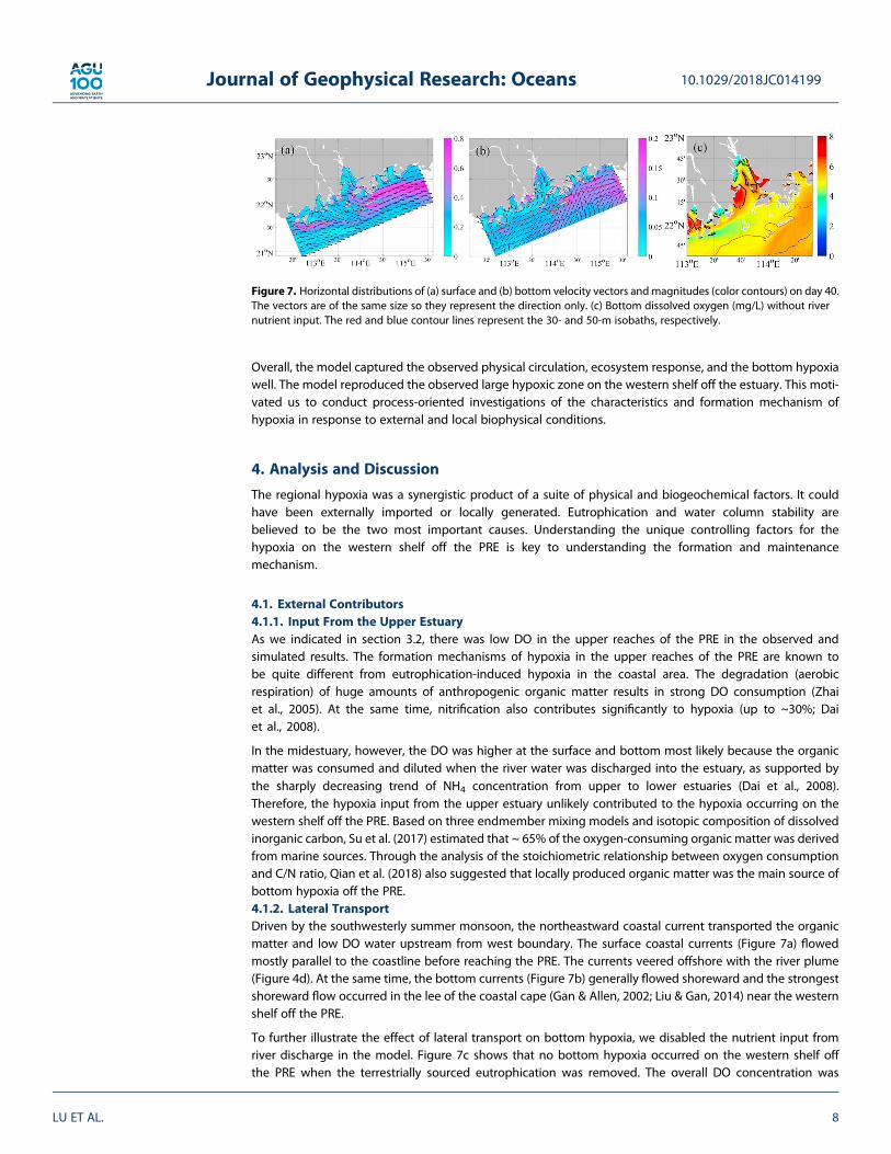
In the midestuary, however, the DO was higher at the surface and bottom most likely because the organicmatter was consumed and diluted when the river water was discharged into the estuary, as supported bythe sharply decreasing trend of NH4 concentration from upper to lower estuaries (Dai et al., 2008).Therefore, the hypoxia input from the upper estuary unlikely contributed to the hypoxia occurring on thewestern shelf off the PRE. Based on three endmember mixing models and isotopic composition of dissolvedinorganic carbon, Su et al. (2017) estimated that ~ 65% of the oxygen-consuming organic matter was derivedfrom marine sources. Through the analysis of the stoichiometric relationship between oxygen consumptionand C/N ratio, Qian et al. (2018) also suggested that locally produced organic matter was the main source ofbottom hypoxia off the PRE.4.1.2. Lateral TransportDriven by the southwesterly summer monsoon, the northeastward coastal current transported the organicmatter and low DO water upstream from west boundary. The surface coastal currents (Figure 7a) flowedmostly parallel to the coastline before reaching the PRE. The currents veered offshore with the river plume(Figure 4d). At the same time, the bottom currents (Figure 7b) generally flowed shoreward and the strongestshoreward flow occurred in the lee of the coastal cape (Gan & Allen, 2002; Liu & Gan, 2014) near the westernshelf off the PRE.

To further illustrate the effect of lateral transport on bottom hypoxia, we disabled the nutrient input fromriver discharge in the model. Figure 7c shows that no bottom hypoxia occurred on the western shelf offthe PRE when the terrestrially sourced eutrophication was removed. The overall DO concentration was

Figure 7. Horizontal distributions of (a) surface and (b) bottom velocity vectors andmagnitudes (color contours) on day 40.The vectors are of the same size so they represent the direction only. (c) Bottom dissolved oxygen (mg/L) without rivernutrient input. The red and blue contour lines represent the 30- and 50-m isobaths, respectively.

10.1029/2018JC014199Journal of Geophysical Research: Oceans

LU ET AL. 8

greater than 4 mg/L. To isolate the key mechanisms and processes better, we then excluded the westernexternal biogeochemical inputs.

4.2. Local Source—Eutrophication

Nutrients are the predominant source contributing to hypoxia development in estuarine and coastal areas(Diaz & Rosenberg, 2008). Excessive nutrient input often leads to an overgrowth of algae that results inhypoxia (Zhu et al., 2016). The intensity and duration of hypoxia are closely related to the nutrient input.However, there is little evidence to suggest that a simple linear response exists between nutrients andhypoxia intensity (Kemp et al., 2009). To assess hypoxia’s response to nutrient loading in the PRE, we variedthe nutrient concentrations in the river in a series of sensitivity experiments.

The most important process for oxygen consumption in the water column and sediment is aerobic respira-tion (equation (A2); Zhai et al., 2005). Nitrification, which typically contains ammonia oxidation and nitrite oxi-dation, is another important process that contributes to oxygen consumption (equation (A3); Dai et al., 2006).The rate of change of DO in the model due to biogeochemical sources and sinks is given by equation (A4)(Fennel et al., 2006). Oxygen consumption due to zooplankton metabolism is relatively small because thezooplankton biomass is generally much smaller than the biomass of phytoplankton and detritus (Ganet al., 2010).

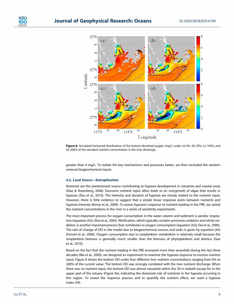
Based on the fact that the nutrient loading in the PRE increased more than sevenfold during the last threedecades (Ma et al., 2009), we designed an experiment to examine the hypoxia response to riverine nutrientinput. Figure 8 shows the bottom DO under four different river nutrient concentrations ranging from 0% to200% of the current value. The bottom DO was strongly correlated with the river nutrient discharge. Whenthere was no nutrient input, the bottom DO was almost saturated within the 30 m isobath except for in theupper part of the estuary (Figure 8a), indicating the dominant role of nutrients in the hypoxia occurring inthis region. To reveal the response process and to quantify the nutrient effect, we used a hypoxiaindex (HI):

Figure 8. Simulated horizontal distributions of the bottom dissolved oxygen (mg/L) under (a) 0%, (b) 50%, (c) 100%, and(d) 200% of the standard nutrient concentration in the river discharge.

10.1029/2018JC014199Journal of Geophysical Research: Oceans

LU ET AL. 9

HI ¼ Vhypoxia� AOU½ �hypoxia (1)

where Vhypoxia is the volume of hypoxic water given by V DO�ð Þ ¼ ∭DO<DO�dxdydz. DO* is the upper limitof the DO concentration for hypoxia (=2 mg/L in this study). [AOU]hypoxia is the mean apparent oxygenutilization of the hypoxic water. AOU is defined by AOU = [O2]eq � [O2], where [O2]eq is the saturatedDO concentration related to in situ temperature and salinity. [O2] is the in situ DO concentration (Zhaiet al., 2005).

In the model, we computed [AOU]hypoxia using AOU½ �hypoxia ¼ 1Vhypoxia

∫ AOU½ �dVhypoxia.

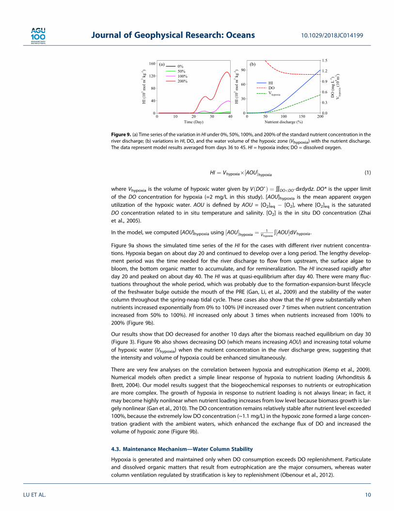
Figure 9a shows the simulated time series of the HI for the cases with different river nutrient concentra-tions. Hypoxia began on about day 20 and continued to develop over a long period. The lengthy develop-ment period was the time needed for the river discharge to flow from upstream, the surface algae tobloom, the bottom organic matter to accumulate, and for remineralization. The HI increased rapidly afterday 20 and peaked on about day 40. The HI was at quasi-equilibrium after day 40. There were many fluc-tuations throughout the whole period, which was probably due to the formation-expansion-burst lifecycleof the freshwater bulge outside the mouth of the PRE (Gan, Li, et al., 2009) and the stability of the watercolumn throughout the spring-neap tidal cycle. These cases also show that the HI grew substantially whennutrients increased exponentially from 0% to 100% (HI increased over 7 times when nutrient concentrationincreased from 50% to 100%). HI increased only about 3 times when nutrients increased from 100% to200% (Figure 9b).

Our results show that DO decreased for another 10 days after the biomass reached equilibrium on day 30(Figure 3). Figure 9b also shows decreasing DO (which means increasing AOU) and increasing total volumeof hypoxic water (Vhypoxia) when the nutrient concentration in the river discharge grew, suggesting thatthe intensity and volume of hypoxia could be enhanced simultaneously.

There are very few analyses on the correlation between hypoxia and eutrophication (Kemp et al., 2009).Numerical models often predict a simple linear response of hypoxia to nutrient loading (Arhonditsis &Brett, 2004). Our model results suggest that the biogeochemical responses to nutrients or eutrophicationare more complex. The growth of hypoxia in response to nutrient loading is not always linear; in fact, itmay become highly nonlinear when nutrient loading increases from low level because biomass growth is lar-gely nonlinear (Gan et al., 2010). The DO concentration remains relatively stable after nutrient level exceeded100%, because the extremely low DO concentration (~1.1 mg/L) in the hypoxic zone formed a large concen-tration gradient with the ambient waters, which enhanced the exchange flux of DO and increased thevolume of hypoxic zone (Figure 9b).

4.3. Maintenance Mechanism—Water Column Stability

Hypoxia is generated and maintained only when DO consumption exceeds DO replenishment. Particulateand dissolved organic matters that result from eutrophication are the major consumers, whereas watercolumn ventilation regulated by stratification is key to replenishment (Obenour et al., 2012).

Figure 9. (a) Time series of the variation in HI under 0%, 50%, 100%, and 200% of the standard nutrient concentration in theriver discharge; (b) variations in HI, DO, and the water volume of the hypoxic zone (Vhypoxia) with the nutrient discharge.The data represent model results averaged from days 36 to 45. HI = hypoxia index; DO = dissolved oxygen.

10.1029/2018JC014199Journal of Geophysical Research: Oceans

LU ET AL. 10

Water column stability is determined by stratification and vertical shear. Stability and shear are indicated by

the Richardson number Ri ¼ �g∂ρ∂zρ ∂u

∂zð Þ2þ ∂v∂zð Þ2

� �, buoyancy frequency BF =ffiffiffiffiffiffiffiffiffiffiffi� g

ρ∂ρ∂z

q, and velocity shear VS = ∂u

∂z

� �2 þ∂v∂z

� �2, where ρ is potential density; g is the gravitational acceleration; z is the vertical coordinate

directed upward; u is the east-west velocity component; and v is the north-south velocity component. A largeRi (>0.25) or BF and a small VS indicate a stable water column (Miles, 1961).

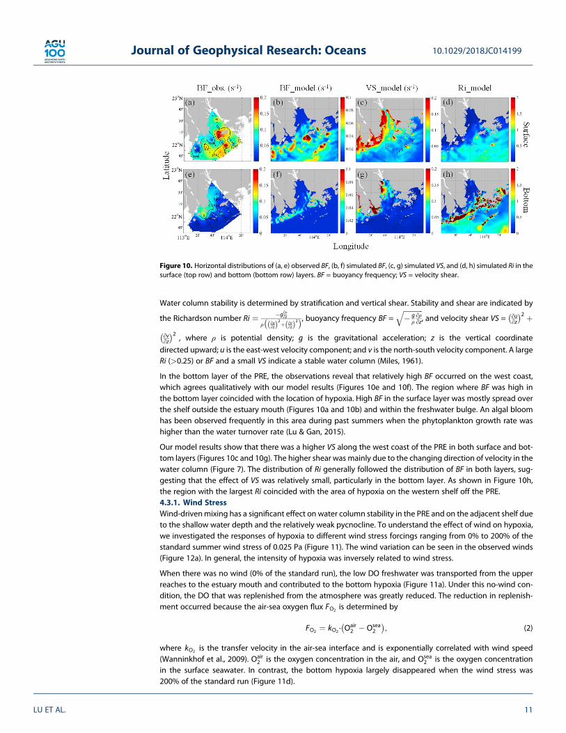
In the bottom layer of the PRE, the observations reveal that relatively high BF occurred on the west coast,which agrees qualitatively with our model results (Figures 10e and 10f). The region where BF was high inthe bottom layer coincided with the location of hypoxia. High BF in the surface layer was mostly spread overthe shelf outside the estuary mouth (Figures 10a and 10b) and within the freshwater bulge. An algal bloomhas been observed frequently in this area during past summers when the phytoplankton growth rate washigher than the water turnover rate (Lu & Gan, 2015).

Our model results show that there was a higher VS along the west coast of the PRE in both surface and bot-tom layers (Figures 10c and 10g). The higher shear was mainly due to the changing direction of velocity in thewater column (Figure 7). The distribution of Ri generally followed the distribution of BF in both layers, sug-gesting that the effect of VS was relatively small, particularly in the bottom layer. As shown in Figure 10h,the region with the largest Ri coincided with the area of hypoxia on the western shelf off the PRE.4.3.1. Wind StressWind-drivenmixing has a significant effect on water column stability in the PRE and on the adjacent shelf dueto the shallow water depth and the relatively weak pycnocline. To understand the effect of wind on hypoxia,we investigated the responses of hypoxia to different wind stress forcings ranging from 0% to 200% of thestandard summer wind stress of 0.025 Pa (Figure 11). The wind variation can be seen in the observed winds(Figure 12a). In general, the intensity of hypoxia was inversely related to wind stress.

When there was no wind (0% of the standard run), the low DO freshwater was transported from the upperreaches to the estuary mouth and contributed to the bottom hypoxia (Figure 11a). Under this no-wind con-dition, the DO that was replenished from the atmosphere was greatly reduced. The reduction in replenish-ment occurred because the air-sea oxygen flux FO2 is determined by

FO2 ¼ kO2 · Oair2 � Osea

2

� �; (2)

where kO2 is the transfer velocity in the air-sea interface and is exponentially correlated with wind speed(Wanninkhof et al., 2009). Oair

2 is the oxygen concentration in the air, and Osea2 is the oxygen concentration

in the surface seawater. In contrast, the bottom hypoxia largely disappeared when the wind stress was200% of the standard run (Figure 11d).

Figure 10. Horizontal distributions of (a, e) observed BF, (b, f) simulated BF, (c, g) simulated VS, and (d, h) simulated Ri in thesurface (top row) and bottom (bottom row) layers. BF = buoyancy frequency; VS = velocity shear.

10.1029/2018JC014199Journal of Geophysical Research: Oceans

LU ET AL. 11

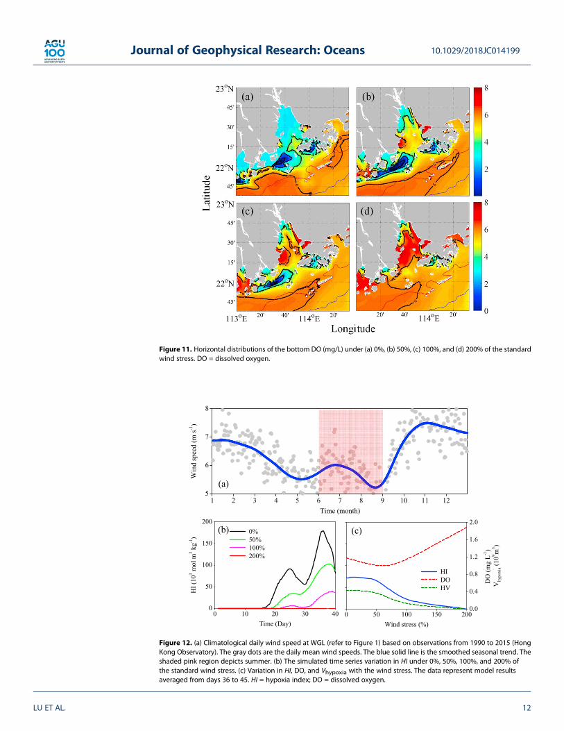
Figure 11. Horizontal distributions of the bottom DO (mg/L) under (a) 0%, (b) 50%, (c) 100%, and (d) 200% of the standardwind stress. DO = dissolved oxygen.

Figure 12. (a) Climatological daily wind speed at WGL (refer to Figure 1) based on observations from 1990 to 2015 (HongKong Observatory). The gray dots are the daily mean wind speeds. The blue solid line is the smoothed seasonal trend. Theshaded pink region depicts summer. (b) The simulated time series variation in HI under 0%, 50%, 100%, and 200% ofthe standard wind stress. (c) Variation in HI, DO, and Vhypoxia with the wind stress. The data represent model resultsaveraged from days 36 to 45. HI = hypoxia index; DO = dissolved oxygen.

10.1029/2018JC014199Journal of Geophysical Research: Oceans

LU ET AL. 12

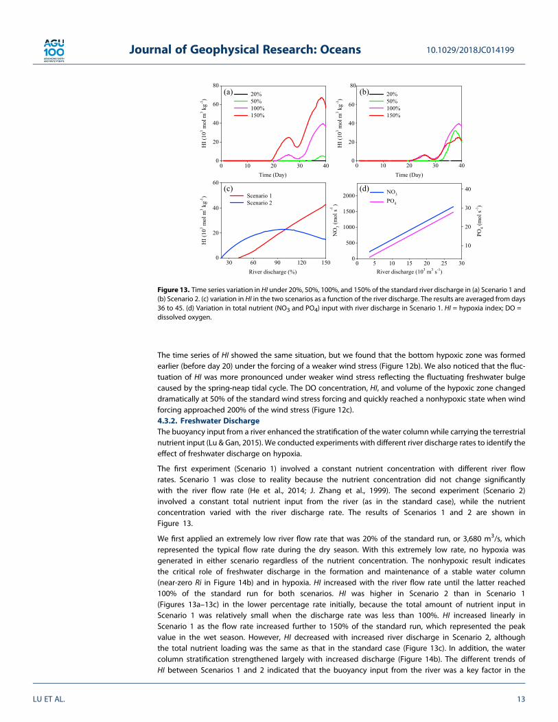
The time series of HI showed the same situation, but we found that the bottom hypoxic zone was formedearlier (before day 20) under the forcing of a weaker wind stress (Figure 12b). We also noticed that the fluc-tuation of HI was more pronounced under weaker wind stress reflecting the fluctuating freshwater bulgecaused by the spring-neap tidal cycle. The DO concentration, HI, and volume of the hypoxic zone changeddramatically at 50% of the standard wind stress forcing and quickly reached a nonhypoxic state when windforcing approached 200% of the wind stress (Figure 12c).4.3.2. Freshwater DischargeThe buoyancy input from a river enhanced the stratification of the water column while carrying the terrestrialnutrient input (Lu & Gan, 2015). We conducted experiments with different river discharge rates to identify theeffect of freshwater discharge on hypoxia.

The first experiment (Scenario 1) involved a constant nutrient concentration with different river flowrates. Scenario 1 was close to reality because the nutrient concentration did not change significantlywith the river flow rate (He et al., 2014; J. Zhang et al., 1999). The second experiment (Scenario 2)involved a constant total nutrient input from the river (as in the standard case), while the nutrientconcentration varied with the river discharge rate. The results of Scenarios 1 and 2 are shown inFigure 13.

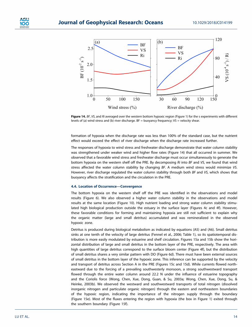
We first applied an extremely low river flow rate that was 20% of the standard run, or 3,680 m3/s, whichrepresented the typical flow rate during the dry season. With this extremely low rate, no hypoxia wasgenerated in either scenario regardless of the nutrient concentration. The nonhypoxic result indicatesthe critical role of freshwater discharge in the formation and maintenance of a stable water column(near-zero Ri in Figure 14b) and in hypoxia. HI increased with the river flow rate until the latter reached100% of the standard run for both scenarios. HI was higher in Scenario 2 than in Scenario 1(Figures 13a–13c) in the lower percentage rate initially, because the total amount of nutrient input inScenario 1 was relatively small when the discharge rate was less than 100%. HI increased linearly inScenario 1 as the flow rate increased further to 150% of the standard run, which represented the peakvalue in the wet season. However, HI decreased with increased river discharge in Scenario 2, althoughthe total nutrient loading was the same as that in the standard case (Figure 13c). In addition, the watercolumn stratification strengthened largely with increased discharge (Figure 14b). The different trends ofHI between Scenarios 1 and 2 indicated that the buoyancy input from the river was a key factor in the

Figure 13. Time series variation in HI under 20%, 50%, 100%, and 150% of the standard river discharge in (a) Scenario 1 and(b) Scenario 2. (c) variation in HI in the two scenarios as a function of the river discharge. The results are averaged from days36 to 45. (d) Variation in total nutrient (NO3 and PO4) input with river discharge in Scenario 1. HI = hypoxia index; DO =dissolved oxygen.

10.1029/2018JC014199Journal of Geophysical Research: Oceans

LU ET AL. 13

formation of hypoxia when the discharge rate was less than 100% of the standard case, but the nutrienteffect would exceed the effect of river discharge when the discharge rate increased further.

The responses of hypoxia to wind stress and freshwater discharge demonstrate that water column stabilitywas strengthened under weaker wind and higher flow rates (Figure 14) that all occurred in summer. Weobserved that a favorable wind stress and freshwater discharge must occur simultaneously to generate thebottom hypoxia on the western shelf off the PRE. By decomposing Ri into BF and VS, we found that windstress affected the water column stability by changing BF. A medium wind stress would minimize VS.However, river discharge regulated the water column stability through both BF and VS, which shows thatbuoyancy affects the stratification and the circulation in the PRE.

4.4. Location of Occurrence—Convergence

The bottom hypoxia on the western shelf off the PRE was identified in the observations and modelresults (Figure 6). We also observed a higher water column stability in the observations and modelresults at the same location (Figure 10). High nutrient loading and strong water column stability stimu-lated high biological production outside the estuary in the surface layer (Figures 4c and 4f). However,these favorable conditions for forming and maintaining hypoxia are still not sufficient to explain whythe organic matter (large and small detritus) accumulated and was remineralized in the observedhypoxic zone.

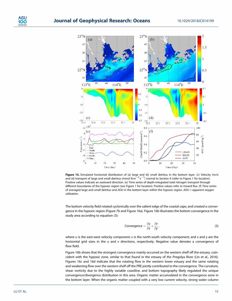
Detritus is produced during biological metabolism as indicated by equations (A5) and (A6). Small detritussinks at one tenth of the velocity of large detritus (Fennel et al., 2006; Table 1), so its spatiotemporal dis-tribution is more easily modulated by estuarine and shelf circulation. Figures 15a and 15b show the hori-zontal distribution of large and small detritus in the bottom layer of the PRE, respectively. The area withhigh quantities of large detritus correspond to the surface bloom center (Figure 4f), but the distributionof small detritus shares a very similar pattern with DO (Figure 6d). There must have been external sourcesof small detritus in the bottom layer of the hypoxic zone. This inference can be supported by the velocityand transport of detritus across Section A in the PRE (Figures 15c and 15d). While currents flowed north-eastward due to the forcing of a prevailing southwesterly monsoon, a strong southwestward transportflowed through the entire water column around 22.2 N under the influence of estuarine topographyand the Coriolis force (Wong, Chen, Xue, Dong, Guan, & Su, 2003a; Wong, Chen, Xue, Dong, Su, &Heinke, 2003b). We observed the westward and southwestward transports of total nitrogen (dissolvedinorganic nitrogen and particulate organic nitrogen) through the eastern and northeastern boundariesof the hypoxic region, indicating the importance of the nitrogen supply through the boundary(Figure 15e). Most of the fluxes entering the region with hypoxia (the box in Figure 1) exited throughthe southern boundary (Figure 15f).

Figure 14. BF, VS, and Ri averaged over the western bottom hypoxic region (Figure 1) for the s experiments with differentlevels of (a) wind stress and (b) river discharge. BF = buoyancy frequency; VS = velocity shear.

10.1029/2018JC014199Journal of Geophysical Research: Oceans

LU ET AL. 14

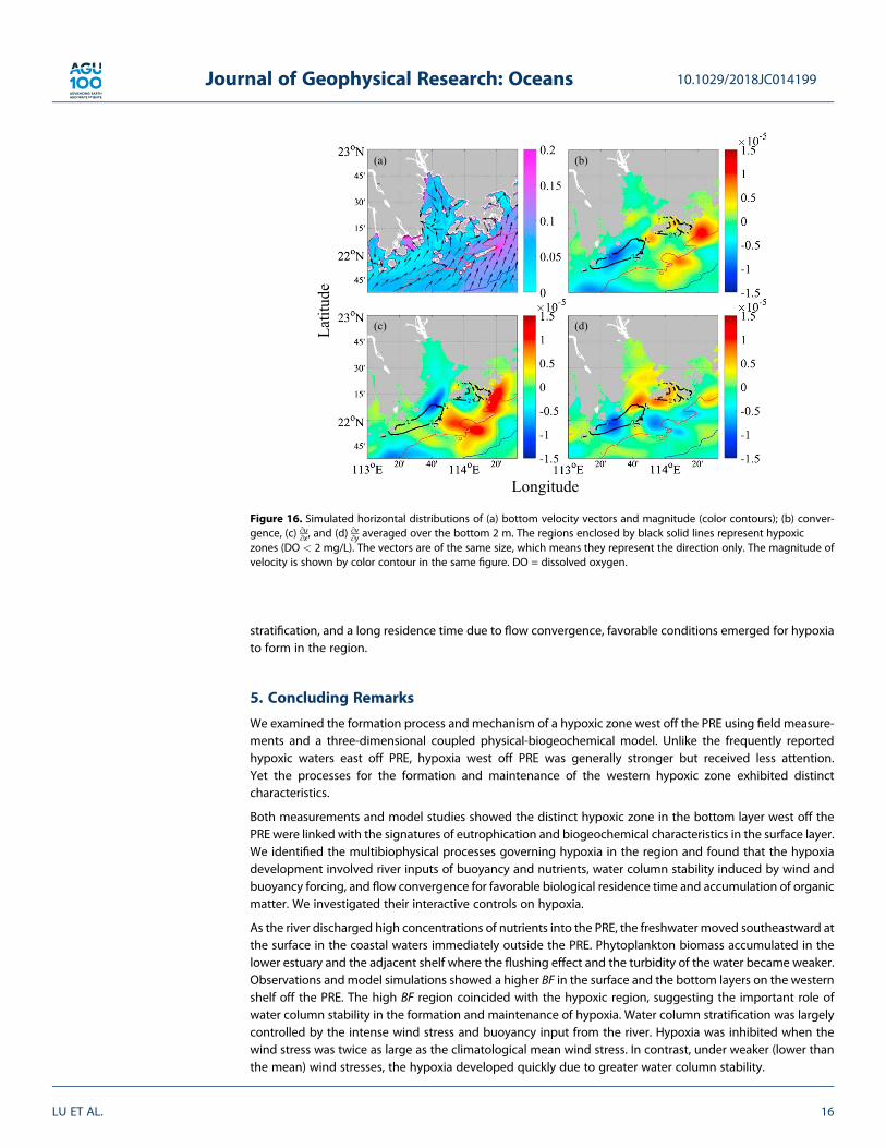
The bottom velocity field rotated cyclonically over the salient edge of the coastal cape, and created a conver-gence in the hypoxic region (Figure 7b and Figure 16a). Figure 16b illustrates the bottom convergence in thestudy area according to equation (3):

Convergence ¼ ∂u∂x

þ ∂v∂y

; (3)

where u is the east-west velocity component; v is the north-south velocity component; and x and y are thehorizontal grid sizes in the u and v directions, respectively. Negative value denotes a convergence offlow field.

Figure 16b shows that the strongest convergence mainly occurred on the western shelf off the estuary, coin-cident with the hypoxic zone, similar to that found in the estuary of the Pregolya River (Lin et al., 2016).Figures 16c and 16d indicate that the rotating flow in the western lower estuary and the same rotatingand weakening flow over the western shelf off the PRE jointly contributed to the convergence. The curvature,shear vorticity due to the highly variable coastline, and bottom topography likely regulated the uniqueconvergence/divergence distribution in this area. Organic matter accumulated in the convergence zone inthe bottom layer. When the organic matter coupled with a very low current velocity, strong water column

Figure 15. Simulated horizontal distribution of (a) large and (b) small detritus in the bottom layer. (c) Velocity (m/s)and (d) transport of large and small detritus (mmol N·m�2·s�1) normal to Section A (refer to Figure 1 for location).Positive values indicate an eastward direction. (e) Time series of depth-integrated total nitrogen transport throughdifferent boundaries of the hypoxic region (see Figure 1 for location). Positive values refer to inward flux. (f) Time seriesof averaged large and small detritus and AOU in the bottom layer within the hypoxic region. AOU = apparent oxygenutilization.

10.1029/2018JC014199Journal of Geophysical Research: Oceans

LU ET AL. 15

stratification, and a long residence time due to flow convergence, favorable conditions emerged for hypoxiato form in the region.

5. Concluding Remarks

We examined the formation process and mechanism of a hypoxic zone west off the PRE using field measure-ments and a three-dimensional coupled physical-biogeochemical model. Unlike the frequently reportedhypoxic waters east off PRE, hypoxia west off PRE was generally stronger but received less attention.Yet the processes for the formation and maintenance of the western hypoxic zone exhibited distinctcharacteristics.

Both measurements and model studies showed the distinct hypoxic zone in the bottom layer west off thePRE were linked with the signatures of eutrophication and biogeochemical characteristics in the surface layer.We identified the multibiophysical processes governing hypoxia in the region and found that the hypoxiadevelopment involved river inputs of buoyancy and nutrients, water column stability induced by wind andbuoyancy forcing, and flow convergence for favorable biological residence time and accumulation of organicmatter. We investigated their interactive controls on hypoxia.

As the river discharged high concentrations of nutrients into the PRE, the freshwater moved southeastward atthe surface in the coastal waters immediately outside the PRE. Phytoplankton biomass accumulated in thelower estuary and the adjacent shelf where the flushing effect and the turbidity of the water became weaker.Observations andmodel simulations showed a higher BF in the surface and the bottom layers on the westernshelf off the PRE. The high BF region coincided with the hypoxic region, suggesting the important role ofwater column stability in the formation and maintenance of hypoxia. Water column stratification was largelycontrolled by the intense wind stress and buoyancy input from the river. Hypoxia was inhibited when thewind stress was twice as large as the climatological mean wind stress. In contrast, under weaker (lower thanthe mean) wind stresses, the hypoxia developed quickly due to greater water column stability.

Figure 16. Simulated horizontal distributions of (a) bottom velocity vectors and magnitude (color contours); (b) conver-gence, (c) ∂u∂x, and (d) ∂v∂y averaged over the bottom 2 m. The regions enclosed by black solid lines represent hypoxiczones (DO < 2 mg/L). The vectors are of the same size, which means they represent the direction only. The magnitude ofvelocity is shown by color contour in the same figure. DO = dissolved oxygen.

10.1029/2018JC014199Journal of Geophysical Research: Oceans

LU ET AL. 16

Freshwater discharge brings large amounts of nutrients for eutrophication in the surface layer and forhypoxia in the bottom layer. In addition, the discharge provides strong buoyancy input which creates a stablewater column for hypoxia to develop and persist. Hypoxia cannot be generated when the river flow rate is toolow even if there is enough nutrient input. We found that the intensity and area of hypoxia grewwith increas-ing river discharge when nutrient concentration was kept constant. However, when we increased river dis-charge (buoyancy) while keeping the total nutrient input unchanged, hypoxia grew with increasing riverdischarge and then weakened after reaching climatological mean value. Stability increased with increasedriver discharge mainly through strengthening stratification (BF) despite an enhanced vertical VS. The windstress regulated the water column’s stability mainly by changing BF, while freshwater discharge achieved thatby additionally changing VS.

The two-layered cyclonically rotating current near the salient edge of the western shelf off the PRE hydrody-namically enhanced the local convergence. The convergence allowed the organic matters produced locallyand remotely sufficient residence time to develop into hypoxia within the region.

In addition to the steady nutrient input from the river, hypoxia was formed and maintained on the westernshelf off the PRE as a result of (1) the stable water column made possible by wind stress and freshwater dis-charge simultaneously and (2) local hydrodynamics favorable for flow convergence and net westward trans-port of organic matter into the region. The first controlling condition was the extrinsic forcing, while thesecond was the intrinsic consequence.

Appendix A: Formulations of Biogeochemical Variables

∂ Phyto½ �∂t

¼ μ Phyto½ � �mp Phyto½ � � τ SDet½ � þ Phyto½ �ð Þ Phyto½ �

� gmaxPhyto½ �2

kPhyto þ Phyto½ �2 Zoo½ � � wPhytow∂ Phyto½ �

∂t;

(A1)

where Phyto, SDet and Zoo represent phytoplankton, small detritus, and zooplankton, respectively. μ, mp, τ,gmax, kPhyto, and wPhyto are the corresponding coefficients for phytoplankton growth rate, phytoplanktonmortality rate, coagulation rate, zooplankton maximum grazing rate, zooplankton half-saturation constantfor ingestion, and the sinking velocity of phytoplankton, respectively.

CH2Oð Þ106 NH3ð Þ16 H3PO4ð Þ þ 138O2 þ 18HCO�3 →

bacteria124CO2 þ 16NO�

3 þ HPO2�4 þ 140H2O (A2)

NHþ4 þ 1:89O2 þ 1:98HCO�

3 →bacteria

0:984NO�3 þ 0:016C5H7O2Nþ 1:90CO2 þ 2:93H2O (A3)

in which, C5H7O2N is the cell stoichiometry for bacteria when phosphorus is excluded.

∂ DO½ �∂t

¼ kprod Phyto½ � � knitri A½ � � kmeta þ kexcretð Þ Zoo½ � � kremin Det½ � þ Flux (A4)

in which A is ammonia, Det is detritus, and Flux is oxygen air-sea flux or other external source/sink(e.g., advection). kprod, knitri, kmeta, kexcret, and kremin are the corresponding coefficients for phytoplanktonproduction, nitrification, zooplankton metabolism, zooplankton excretion, and detritus remineralization,respectively.

∂ LDN½ �∂t

¼ τ SDN½ � þ Phyto½ �ð Þ2 � rLDN LDN½ � � wLD∂ LDN½ �∂z

(A5)

∂ SDN½ �∂t

¼ gmaxPhyto½ �2

kPhyto þ Phyto½ �2 1� βð Þ Zoo½ � þmZoo Zoo½ �2

þ mPhyto Phyto½ � � τ SDN½ � þ Phyto½ �ð Þ SDN½ � � rSDN SDN½ � � wSD∂ SDN½ �∂z

;

(A6)

10.1029/2018JC014199Journal of Geophysical Research: Oceans

LU ET AL. 17

where LDN and SDN represent N fraction of large and small detritus, respectively; rLDN and rSDN are the remi-neralization rate for N fraction of large and small detritus, respectively; wLd andwSD are the sinking velocity oflarge and small detritus, respectively; β is the zooplankton assimilation efficiency; and mZoo is the zooplank-ton mortality rate.

ReferencesArhonditsis, G. B., & Brett, M. T. (2004). Evaluation of the current state of mechanistic aquatic biogeochemical modeling. Marine Ecology

Progress Series, 271, 13–26. https://doi.org/10.3354/meps271013Bianchi, T. S., DiMarco, S. F., Cowan, J. H., Hetland, R. D., Chapman, P., Day, J. W., & Allison, M. A. (2010). The science of hypoxia in the northern

Gulf of Mexico: A review. Science of the Total Environment, 408(7), 1471–1484. https://doi.org/10.1016/j.scitotenv.2009.11.047Breitburg, D., Levin, L. A., Oschlies, A., Gregoire, M., Chavez, F. P., Conley, D. J., et al. (2018). Declining oxygen in the global ocean and coastal

waters. Science, 359(6371), 46.Bryan, J. R., Riley, J. P., & Williams, P. J. (1976). A winkler procedure for making precise measurements of oxygen concentration for produc-

tivity and related studies. Journal of Experimental Marine Biology and Ecology, 21(3), 191–197.Cai, W. J., Dai, M. H., Wang, Y. C., Zhai, W. D., Huang, T., Chen, S. T., et al. (2004). The biogeochemistry of inorganic carbon and nutrients in the

Pearl River estuary and the adjacent northern South China Sea. Continental Shelf Research, 24(12), 1301–1319. https://doi.org/10.1016/j.csr.2004.04.005

Cai, W. J., Hu, X. P., Huang, W. J., Murrell, M. C., Lehrter, J. C., Lohrenz, S. E., et al. (2011). Acidification of subsurface coastal waters enhanced byeutrophication. Nature Geoscience, 4(11), 766–770. https://doi.org/10.1038/Ngeo1297

Callahan, J., Dai, M. H., Chen, R. F., Li, X. L., Lu, Z. M., & Huang, W. (2004). Distribution of dissolved organic matter in the Pearl River estuary,China. Marine Chemistry, 89(1–4), 211–224. https://doi.org/10.1016/j.marchem.2004.02.013

Chu, P., Chen, Y. C., & Kuninaka, A. (2005). Seasonal variability of the Yellow Sea/East China Sea surface fluxes and thermohaline structure.Advances in Atmospheric Sciences, 22(1), 1–20. https://doi.org/10.1007/BF02930865

Dagg, M. J., Ammerman, J. W., Amon, R. M. W., Gardner, W. S., Green, R. E., & Lohrenz, S. E. (2007). A review of water column processesinfluencing hypoxia in the northern Gulf of Mexico. Estuaries and Coasts, 30(5), 735–752. https://doi.org/10.1007/BF02841331

Dai, M. H., Guo, X. G., Zhai, W. D., Yuan, L. Y., Wang, B. W., Wang, L. F., et al. (2006). Oxygen depletion in the upper reach of the Pearl Riverestuary during a winter drought. Marine Chemistry, 102(1–2), 159–169. https://doi.org/10.1016/j.marchem.2005.09.020

Dai, M. H., Wang, L., Guo, X., Zhai, W., Li, Q., He, B., & Kao, S. J. (2008). Nitrification and inorganic nitrogen distribution in a large perturbedriver/estuarine system: The Pearl River estuary, China. Biogeosciences, 5(5), 1227–1244. https://doi.org/10.5194/bg-5-1227-2008

Dai, M. H., Gan, J. P., Han, A., Kung, H. S., & Yin, Z. Q. (2014). Physical dynamics and biogeochemistry of the Pearl River plume. In T. Bianchi,M. Allison, & W.-J. Cai (Eds.), Biogeochemical Dynamics at Major River-Coastal Interfaces: Linkages with Global Change. Cambridge:Cambridge University Press.

Diaz, R. J., & Rosenberg, R. (2008). Spreading dead zones and consequences for marine ecosystems. Science, 321(5891), 926–929. https://doi.org/10.1126/science.1156401

Fennel, K., Wilkin, J., Levin, J., Moisan, J., O’Reilly, J., & Haidvogel, D. (2006). Nitrogen cycling in the middle Atlantic bight: Results from a three-dimensional model and implications for the North Atlantic nitrogen budget. Global Biogeochemical Cycles, 20, GB3007. https://doi.org/10.1029/2005GB002456

Gan, J., & Allen, J. S. (2002). A modeling study of shelf circulation off northern California in the region of the Coastal Ocean dynamicsexperiment: Response to relaxation of upwelling winds. Journal of Geophysical Research, 107(C11), 3184. https://doi.org/10.1029/2001JC001190

Gan, J., & Allen, J. S. (2005). On open boundary conditions for a limited-area coastal model off Oregon. Part 2: Response to wind forcing froma regional mesoscale atmospheric model. Ocean Modelling, 8(1–2), 155–173. https://doi.org/10.1016/j.ocemod.2003.12.007

Gan, J., Cheung, A., Guo, X. G., & Li, L. (2009). Intensified upwelling over a widened shelf in the northeastern South China Sea. Journal ofGeophysical Research, 114, C09019. https://doi.org/10.1029/2007JC004660

Gan, J., Li, L., Wang, D. X., & Guo, X. G. (2009). Interaction of a river plume with coastal upwelling in the northeastern South China Sea.Continental Shelf Research, 29(4), 728–740. https://doi.org/10.1016/j.csr.2008.12.002

Gan, J., Lu, Z. M., Dai, M. H., Cheung, A., Harrison, P., & Liu, H. B. (2010). Biological response to intensified upwelling and to a river plume in thenortheastern South China Sea: A modeling study. Journal of Geophysical Research, 115, C09001. https://doi.org/10.1029/2009JC005569

Gan, J. P., Lu, Z. M., Cheung, A., Dai, M., Liang, L. L., Harrison, P. J., & Zhao, X. Z. (2014). Assessing ecosystem response to phosphorus andnitrogen limitation in the Pearl River plume using the Regional Ocean Modeling System (ROMS). Journal of Geophysical Research: Oceans,119, 8858–8877. https://doi.org/10.1002/2014JC009951

Hagy, J. D., Boynton, W. R., Keefe, C. W., & Wood, K. V. (2004). Hypoxia in Chesapeake Bay, 1950–2001: Long-term change in relation tonutrient loading and river flow. Estuaries, 27(4), 634–658. https://doi.org/10.1007/Bf02907650

Harrison, P. J., Yin, K. D., Lee, J. H. W., Gan, J. P., & Liu, H. B. (2008). Physical-biological coupling in the Pearl River estuary. Continental ShelfResearch, 28(12), 1405–1415. https://doi.org/10.1016/j.csr.2007.02.011

He, B. Y., Dai, M. H., Zhai, W. D., Guo, X. H., & Wang, L. F. (2014). Hypoxia in the upper reaches of the Pearl River estuary and its maintenancemechanisms: A synthesis based on multiple year observations during 2000–2008.Marine Chemistry, 167, 13–24. https://doi.org/10.1016/j.marchem.2014.07.003

He, B. Y., Dai, M. H., Zhai, W. D., Wang, L. F., Wang, K. J., Chen, J. H., et al. (2010). Distribution, degradation and dynamics of dissolved organiccarbon and its major compound classes in the Pearl River estuary, China. Marine Chemistry, 119(1–4), 52–64. https://doi.org/10.1016/j.marchem.2009.12.006

Helly, J. J., & Levin, L. A. (2004). Global distribution of naturally occurring marine hypoxia on continental margins. Deep-Sea Research Part I,51(9), 1159–1168. https://doi.org/10.1016/j.dsr.2004.03.009

Huang, X. P., Huang, L. M., & Yue, W. Z. (2003). The characteristics of nutrients and eutrophication in the Pearl River estuary, South China.Marine Pollution Bulletin, 47(1–6), 30–36. https://doi.org/10.1016/S0025-326x(02)00474-5

Kemp, W. M., Testa, J. M., Conley, D. J., Gilbert, D., & Hagy, J. D. (2009). Temporal responses of coastal hypoxia to nutrient loading and physicalcontrols. Biogeosciences, 6(12), 2985–3008. https://doi.org/10.5194/bg-6-2985-2009

Lin, P. G., Hu, J. Y., Zheng, Q. A., Sun, Z. Y., & Zhu, J. (2016). Observation of summertime upwelling off the eastern and northeastern coasts ofHainan Island, China. Ocean Dynamics, 66(3), 387–399. https://doi.org/10.1007/s10236-016-0934-2

10.1029/2018JC014199Journal of Geophysical Research: Oceans

LU ET AL. 18

AcknowledgmentsThis research was supported by theTheme-based Research Scheme (T21-602/16-R) of the Hong Kong ResearchGrants Council. We are grateful for thesupport of The NationalSupercomputing Center of Tianjin andGuangzhou. All of the numericalinformation provided in the figures wasproduced by solving equations in theROMS. The source code of ROMS can bedownloaded from https://www.myroms.org/ and data used in the paperare provided in the supportinginformation.

Liu, Z., & Gan, J. (2014). Modeling study of variable upwelling circulation in the East China Sea: Response to a coastal promontory. Journal ofPhysical Oceanography, 44(4), 1078–1094. https://doi.org/10.1175/JPO-D-13-0170.1

Lu, Z. M., & Gan, J. P. (2015). Controls of seasonal variability of phytoplankton blooms in the Pearl River estuary. Deep-Sea Research Part II, 117,86–96.

Luo, L., Li, S., & Wang, D. (2009). Hypoxia in the Pearl River estuary, the South China Sea, in July 1999. Aquatic Ecosystem Health, 12(4), 418–428.https://doi.org/10.1080/14634980903352407

Ma, Y., Wei, W., Xia, H. Y., Yu, B., Wang, D., Ma, Y., & Wang, L. (2009). History change and influence factor of nutrient in Lingdinyang Sea area ofZhujiang River Eestuary (in Chinese with English abstract). Acta Oceanologica Sinica, 31(2), 69–77.

Miles, J. W. (1961). On the stability of heterogeneous shear flows. Journal of Fluid Mechanics, 10(04), 496–508. https://doi.org/10.1017/S0022112061000305

Obenour, D. R., Michalak, A. M., Zhou, Y. T., & Scavia, D. (2012). Quantifying the impacts of stratification and nutrient loading on hypoxia in thenorthern Gulf of Mexico. Environmental Science & Technology, 46(10), 5489–5496. https://doi.org/10.1021/es204481a

Parsons, T. R., Maita, Y., & Lalli, C. M. (1984). A manual of chemical and biological methods for seawater analysis. Oxford: Pergamon Press.Qian, W., Gan, J. P., Liu, J. W., He, B. Y., Lu, Z. M., Guo, X. H., et al. (2018). Current status of emerging hypoxia in a eutrophic estuary: The lower

reach of the Pearl River estuary, China. Estuarine, Coastal and Shelf Science, 205, 58–67. https://doi.org/10.1016/j.ecss.2018.03.004Rabalais, N. N., Cai, W. J., Carstensen, J., Conley, D. J., Fry, B., Hu, X. P., et al. (2014). Eutrophication-driven deoxygenation in the coastal ocean.

Oceanography, 27(1), 172–183. https://doi.org/10.5670/oceanog.2014.21Rabalais, N. N., Diaz, R. J., Levin, L. A., Turner, R. E., Gilbert, D., & Zhang, J. (2010). Dynamics and distribution of natural and human-caused

hypoxia. Biogeosciences, 7(2), 585–619. https://doi.org/10.5194/bg-7-585-2010Rabalais, N. N., Turner, R. E., & Wiseman, W. J. (2002). Gulf of Mexico hypoxia, aka “the dead zone”. Annual Review of Ecology and Systematics,

33(1), 235–263. https://doi.org/10.1146/annurev.ecolsys.33.010802.150513Rabouille, C., Conley, D. J., Dai, M. H., Cai, W. J., Chen, C. T. A., Lansard, B., et al. (2008). Comparison of hypoxia among four river-dominated

ocean margins: The Changjiang (Yangtze), Mississippi, Pearl, and Rhone rivers. Continental Shelf Research, 28(12), 1527–1537. https://doi.org/10.1016/j.csr.2008.01.020

Shchepetkin, A. F., & McWilliams, J. C. (2005). The Regional Oceanic Modeling System (ROMS): A split-explicit, free-surface, topography-following-coordinate oceanic model. Ocean Modelling, 9(4), 347–404. https://doi.org/10.1016/j.ocemod.2004.08.002

Spitz, Y. H., Allen, J. S., & Gan, J. (2005). Modeling of ecosystem processes on the Oregon shelf during the 2001 summer upwelling. Journal ofGeophysical Research, 110, C10S17. https://doi.org/10.1029/2005JC002870

Su, J. Z., Dai, M. H., He, B. Y., Wang, L. F., Gan, J. P., Guo, X. H., et al. (2017). Tracing the origin of the oxygen-consuming organic matter in thehypoxic zone in a large eutrophic estuary: The lower reach of the Pearl River estuary, China. Biogeosciences, 14(18), 4085–4099. https://doi.org/10.5194/bg-14-4085-2017

Swarzenski, P. W., Campbell, P. L., Osterman, L. E., & Poore, R. Z. (2008). A 1000-year sediment record of recurring hypoxia off the MississippiRiver: The potential role of terrestrially-derived organic matter inputs. Marine Chemistry, 109(1–2), 130–142. https://doi.org/10.1016/j.marchem.2008.01.003

Turner, R. E., & Rabalais, N. N. (1994). Coastal eutrophication near the Mississippi River Delta. Nature, 368(6472), 619–621. https://doi.org/10.1038/368619a0

Wang, B., Hu, J. T., Li, S. Y., & Liu, D. H. (2017). A numerical analysis of biogeochemical controls with physical modulation on hypoxia duringsummer in the Pearl River estuary. Biogeosciences, 14(12), 2979–2999. https://doi.org/10.5194/bg-14-2979-2017

Wang, H. J., Dai, M. H., Liu, J. W., Kao, S. J., Zhang, C., Cai, W. J., et al. (2016). Eutrophication-driven hypoxia in the East China Sea off theChangjiang estuary. Environmental Science & Technology, 50(5), 2255–2263. https://doi.org/10.1021/acs.est.5b06211

Wang, L. X., & Justic, D. (2009). A modeling study of the physical processes affecting the development of seasonal hypoxia over the innerLouisiana-Texas shelf: Circulation and stratification. Continental Shelf Research, 29(11–12), 1464–1476. https://doi.org/10.1016/j.csr.2009.03.014

Wanninkhof, R., Asher, W. E., Ho, D. T., Sweeney, C., & McGillis, W. R. (2009). Advances in quantifying air-sea gas exchange and environmentalforcing. Annual Review of Marine Science, 1(1), 213–244. https://doi.org/10.1146/annurev.marine.010908.163742

Wei, X., Zhan, H. G., Ni, P. T., & Cai, S. Q. (2016). A model study of the effects of river discharges and winds on hypoxia in summer in the PearlRiver estuary. Marine Pollution Bulletin, 113(1–2), 414–427. https://doi.org/10.1016/j.marpolbul.2016.10.042

Wiseman, W. J., Rabalais, N. N., Turner, R. E., Dinnel, S. P., & MacNaughton, A. (1997). Seasonal and interannual variability within the Louisianacoastal current: Stratification and hypoxia. Journal of Marine Systems, 12(1–4), 237–248. https://doi.org/10.1016/S0924-7963(96)00100-5

Wong, L. A., Chen, J., Xue, H., Dong, L. X., Su, J. L., & Heinke, G. (2003b). A model study of the circulation in the Pearl River estuary (PRE) and itsadjacent coastal waters: 1. Simulations and comparison with observations. Journal of Geophysical Research, 108(C5), 3156. https://doi.org/10.1029/2002JC001451

Wong, L. A., Chen, J. C., Xue, H., Dong, L. X., Guan, W. B., & Su, J. L. (2003a). A model study of the circulation in the Pearl River estuary (PRE) andits adjacent coastal waters: 2. Sensitivity experiments. Journal of Geophysical Research, 108(C5), 3157. https://doi.org/10.1029/2002JC001452

Yin, K. D., Lin, Z. F., & Ke, Z. Y. (2004). Temporal and spatial distribution of dissolved oxygen in the Pearl River estuary and adjacent coastalwaters. Continental Shelf Research, 24(16), 1935–1948. https://doi.org/10.1016/j.csr.2004.06.017

Zhai, W., Dai, M., Cai, W.-J., Wang, Y., & Wang, Z. (2005). High partial pressure of CO2 and its maintaining mechanism in a subtropical estuary:The Pearl River estuary, China. Marine Chemistry, 93(1), 21–32. https://doi.org/10.1016/j.marchem.2004.07.003

Zhang, F. (2001). Seasonal variation features of chlorophyll a content in Taiwan Strait (in Chinese with English abstract). Journal ofOceanography in Taiwan Strait, 20(3), 314–318.

Zhang, H., & Li, S. Y. (2010). Effects of physical and biochemical processes on the dissolved oxygen budget for the Pearl River estuary duringsummer. Journal of Marine Systems, 79(1–2), 65–88. https://doi.org/10.1016/j.jmarsys.2009.07.002

Zhang, J., Gilbert, D., Gooday, A. J., Levin, L., Naqvi, S. W. A., Middelburg, J. J., et al. (2010). Natural and human-induced hypoxia and conse-quences for coastal areas: Synthesis and future development. Biogeosciences, 7(5), 1443–1467. https://doi.org/10.5194/bg-7-1443-2010

Zhang, J., Yu, Z. G., Wang, J. T., Ren, J. L., Chen, H. T., Xiong, H., et al. (1999). The subtropical Zhujiang (Pearl River) estuary: Nutrient, tracespecies and their relationship to photosynthesis. Estuarine and Coastal Marine Science, 49(3), 385–400. https://doi.org/10.1006/ecss.1999.0500

Zhu, J. R., Zhu, Z. Y., Lin, J., Wu, H., & Zhang, J. (2016). Distribution of hypoxia and pycnocline off the Changjiang estuary, China. Journal ofMarine Systems, 154, 28–40. https://doi.org/10.1016/j.jmarsys.2015.05.002

Zu, T., & Gan, J. (2015). A numerical study of coupled estuary-shelf circulation around the Pearl River estuary during summer: Responses tovariable winds, tides and river discharge. Deep-Sea Research Part II, 117, 53–64. https://doi.org/10.1016/j.dsr1012.2013.1012.1010

10.1029/2018JC014199Journal of Geophysical Research: Oceans

LU ET AL. 19