­2 ­1 0 1 2 3 4 50

0.02

0.04

0.06

0.08

0.1

0.12

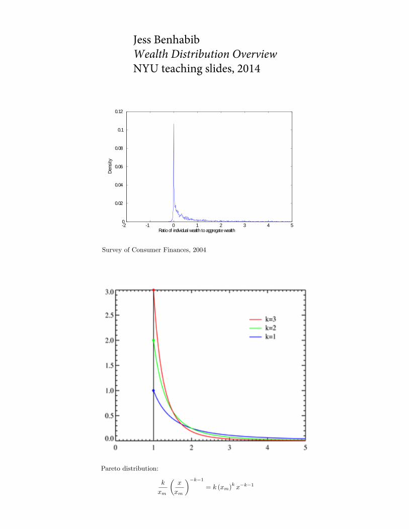
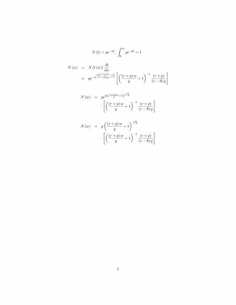
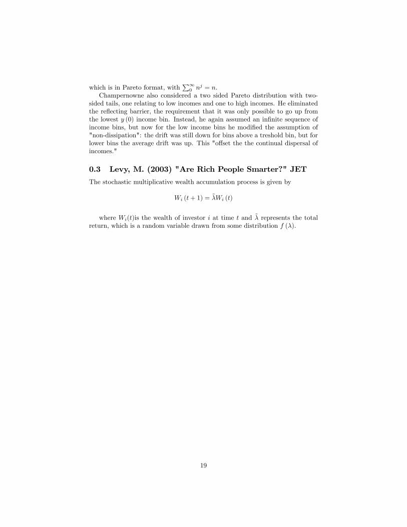
Ratio of individual wealth to aggregate wealth

Dens

ity

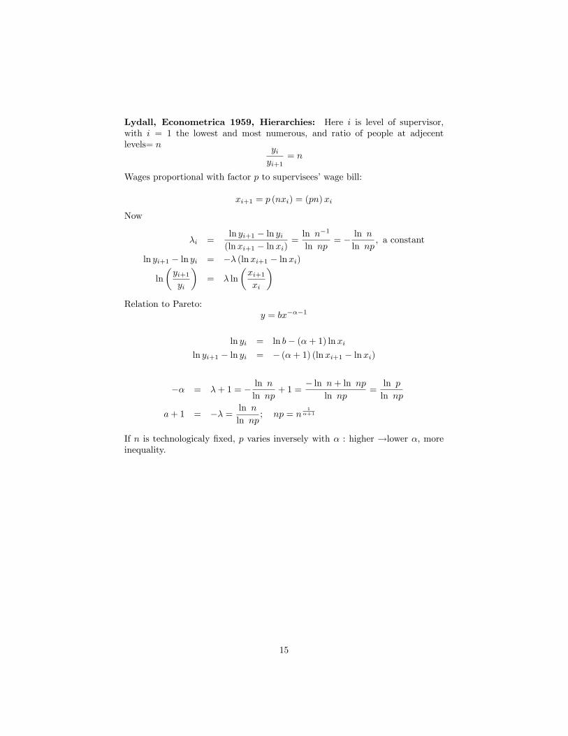
Survey of Consumer Finances, 2004

1

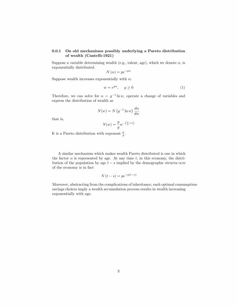
Pareto distribution:

k

xm

(x

xm

)−k−1= k (xm)

kx−k−1

Jess BenhabibWealth Distribution OverviewNYU teaching slides, 2014

0.0.1 On old mechanisms possibly underlying a Pareto distributionof wealth (Cantelli-1921)

Suppose a variable determining wealth (e.g., talent, age), which we denote α, isexponentially distributed.

N (α) = pe−pα

Suppose wealth increases exponentially with α:

w = egα, g ≥ 0 (1)

Therefore, we can solve for α = g−1 lnw, operate a change of variables andexpress the distribution of wealth as

N(w) = N(g−1 lnw

) dαdw

that is,N(w) =

p

gw−( pg+1)

It is a Pareto distribution with exponent pg .

3

A similar mechanism which makes wealth Pareto distributed is one in whichthe factor α is represented by age. At any time t, in this economy, the distri-bution of the population by age t− s implied by the demographic structu-∞reof the economy is in fact

N (t− s) = pe−p(t−s)

Moreover, abstracting from the complications of inheritance, each optimal consumption-savings choices imply a wealth accumulation process results in wealth increasingexponentially with age.

Frechet (1939) Use Laplace distribution for talents/skills:

N (s) = e−a|s|, s = (−∞,+∞)

Income:

w = ebs, s = b−1 lnw

ds

sw= b−1

1

w

Edgeworth translation technique:

N (w) = b−11

we−a|

lnwb | =

b−1 1we− ab lnw if w ≥ 1

b−1 1weab lnw if w ≤ 1

=b−1w−

ab−1 if w ≥ 1

b−1wab−1 if w ≤ 1

Note: for w ≤ 1, N (w) is increasing

5

Pareto in Blanchard’s Model Here θ is the discount rate, p is the constantdeath probability and also the fair annuity premium, r is the return on wealth.For wealth to remain bounded a standard assumption (See Blanchard (JPE,1985)) is r < p+ θ, where p+ θ is the effective augmented discount rate of theagent with constant death probability p.

w = (r + p)w + y − cc (s, t) = (p+ θ) (w + h)

h =

∫ ∞t

y (s, v) e∫ vt(r(u)+p)dudv

h = y

∫ ∞t

e−(r+p)(v−t)dv = −y (r + p)−1e−(r+p)(v−t)|∞t

= y (r + p)−1

w = (r + p)w + y − (p+ θ) (w + h)

= (r − θ)w + y − (p+ θ)h

= (r − θ)w + y − (p+ θ) y (r + p)−1

= (r − θ)w + y

(r − θr + p

)

w (t) =

(w (0) +

y

r + p

)e(r−θ)t − y

r + p

so for large w the agent wealth grows at rate r − θ. If w (0) = 0, t is age:

w (t) =

(y

r + p

)e(r−θ)t − y

r + p

=y

r + p

(e(r−θ)t − 1

)

w (t) +y

r + p=

(y

r + p

)e(r−θ)t

ln

(w (t) (r + p)

y+ 1

)= (r − θ) t

t =ln((r+p)w

y + 1)

r − θTransform variables:

dt

dw= (r − θ)−1

((r + p)w

y+ 1

)−1(r + p)

y

6

N (t) = pe−pt,

∫ ∞0

pe−pt = 1

N (w) = N (t (w))dt

dw

= pe−pln( (r+p)wy

+1)r−θ

[((r + p)w

y+ 1

)−1(r + p)

(r − θ) y

]

N (w) = peln((r+p)w

y +1)−pr−θ

·[(

(r + p)w

y+ 1

)−1(r + p)

(r − θ) y

]

N (w) = p

((r + p)w

y+ 1

) −pr−θ

·[(

(r + p)w

y+ 1

)−1(r + p)

(r − θ) y

]

7

Pareto density in W = (r+p)wy + 1 :

N (w) =

[p (r + p)

(r − θ) y

]((r + p)w

y+ 1

) −pr−θ−1

N (0) =

[p (r + p)

(r − θ) y

]with Pareto exponent p

r−θ . It is greater than 1 under the assumption r < p+ θ.Check that population integrates to 1:

∫ ∞0

N (w) dw

=

[p (r + p)

(r − θ) y

] [(−r − θ

p

)(y

r + p

)((r + p)w

y+ 1

) −pr−θ]∞0

=

[p (r + p)

(r − θ) y

](y

r + p

)(r − θp

)= 1

If we allow incomes y to grow over time at rate g, and discount wealth by g,then the Pareto exponent becomes p

((r−g)−θ) .

8

0.1 Multiplicative Talent (Roy-1950)

Incomes w are linearly dependent on talent S;

w = aS

Talent is the product of attributes, si whereeach attribute is drawn from an iiddistribution.

w = as1s2...sn

lnw = ln a+ ln s1 + ln s2...+ ln sn

So incomes are log linear. You can also study skewness when the si are notindependent.

9

0.1.1 Kalecki (1945)

Idea: Kill random walk or variance exploding: make random return depend onfirm size.Let deviation of firm size, Xi

t+1 = RitXit where R

it is a random variable. In

logs

lnXit+1 = lnXi

t + lnRit = lnXi0 +

t∑j=0

lnRij

so lnXt+1 is approximately normal. Assume variance of firm size remains con-stant.

1

n

∑i

(lnXi

t + lnRit)2

=1

n

∑i

(lnXi

t

)2= M

2∑i

(lnXi

t lnRit)

= −∑i

(lnRit

)2and we may assume a negative linear relation

lnRt = −α lnXt + z,

α =

∑(lnRit

)22∑(

lnXit

)2 , z iid∑i

(lnXi

t lnRit)

= −α∑i

(lnXi

t

)2= −

∑(lnRit

)22∑(

lnXit

)2 ∑i

(lnXi

t

)2∑i

(lnXi

t lnRit)

= −1

2

∑(lnRit

)2Then the limiting distribution is normal:

lnXit+1 = (1− α) lnXi

t+1 + z; X∞ = α−1z

10

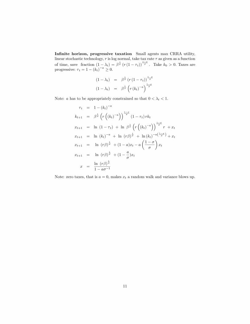
Infinite horizon, progressive taxation Small agents max CRRA utility,linear stochastic technology, r is log normal, take tax rate τ as given as a function

of time, save fraction (1− λt) = β1σ (r (1− τ t))

1−σσ . Take k0 > 0. Taxes are

progressive: τ t = 1− (kt)−a ≥ 0.

(1− λt) = β1σ (r (1− τ t))

1 σσ

(1− λt) = β1σ

(r (kt)

−a) 1−σ

σ

Note: a has to be appropriately constrained so that 0 < λt < 1.

τ t = 1− (kt)−a

kt+1 = β1σ

(r(

(kt)−a)) 1−σ

σ

(1− τ t) rkt

xt+1 = ln (1− τ t) + ln β1σ

(r(

(kt)−a)) 1−σ

σ

r + xt

xt+1 = ln (kt)−a

+ ln (rβ)1σ + ln (kt)

−a( 1−σσ ) + xt

xt+1 = ln (rβ)1σ + (1− a)xt − a

(1− σσ

)xt

xt+1 = ln (rβ)1σ + (1− a

σ)xt

x =ln (rβ)

1σ

1− aσ−1

Note: zero taxes, that is a = 0, makes xt a random walk and variance blows up.

11

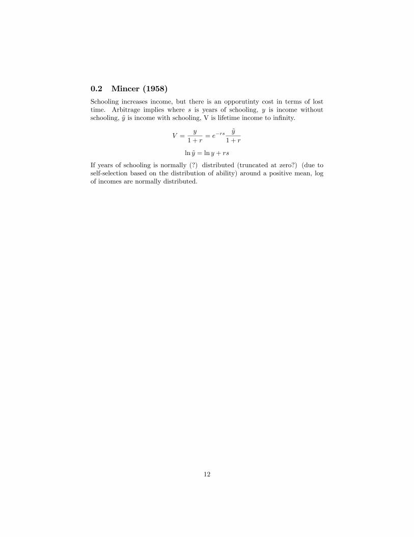
0.2 Mincer (1958)

Schooling increases income, but there is an opporutinty cost in terms of losttime. Arbitrage implies where s is years of schooling, y is income withoutschooling, y is income with schooling, V is lifetime income to infinity.

V =y

1 + r= e−rs

y

1 + r

ln y = ln y + rs

If years of schooling is normally (?) distributed (truncated at zero?) (due toself-selection based on the distribution of ability) around a positive mean, logof incomes are normally distributed.

12

In many cases, the theoretical modeling of the wealth distribution got verymechanical, and engineering or physics-like in fact, leading Mincer (1958) toplead for explicit microfoundations and more explicit determinants of earningsand wealth distributions:

From the economist’s point of view, perhaps the most unsatisfactoryfeature of the stochastic models, which they share with most othermodels of personal income distribution, is that they shed no lighton the economics of the distribution process. Non-economic factorsundoubtedly play an important role in the distribution of incomes.Yet, unless one denies the relevance of rational optimizing behaviorto economic activity in general, it is diffi cult to see how the factor ofindividual choice can be disregarded in analyzing personal incomedistribution, which can scarcely be independent of economic activity.

13

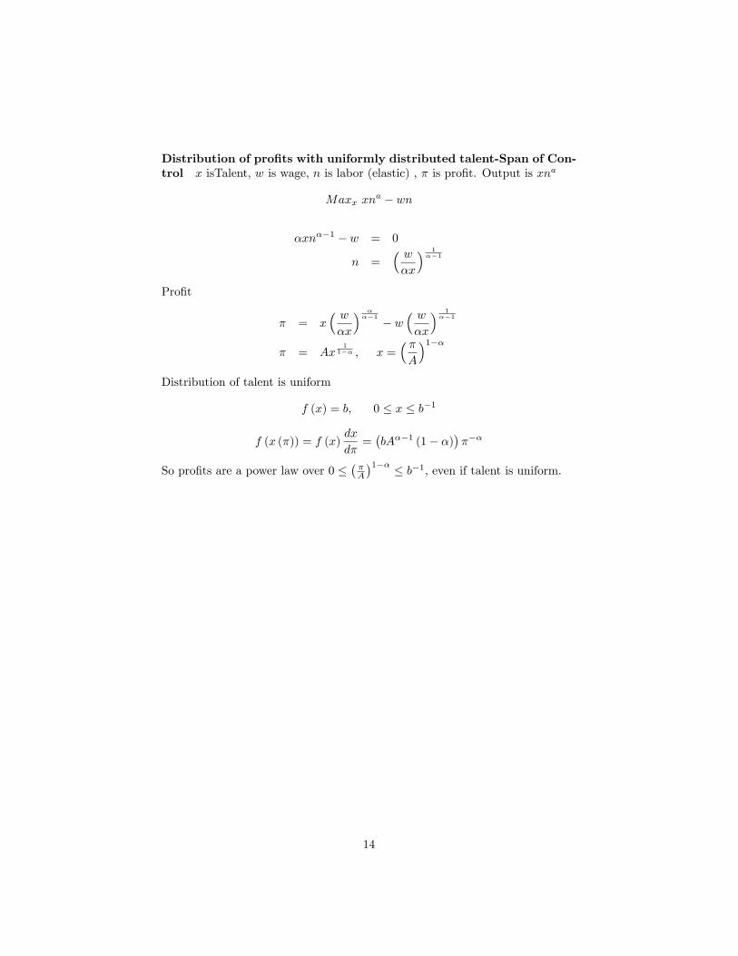
Distribution of profits with uniformly distributed talent-Span of Con-trol x isTalent, w is wage, n is labor (elastic) , π is profit. Output is xna

Maxx xna − wn

αxnα−1 − w = 0

n =( wαx

) 1α−1

Profit

π = x( wαx

) αα−1 − w

( wαx

) 1α−1

π = Ax1

1−α , x =( πA

)1−αDistribution of talent is uniform

f (x) = b, 0 ≤ x ≤ b−1

f (x (π)) = f (x)dx

dπ=(bAα−1 (1− α)

)π−α

So profits are a power law over 0 ≤(πA

)1−α ≤ b−1, even if talent is uniform.

14

Lydall, Econometrica 1959, Hierarchies: Here i is level of supervisor,with i = 1 the lowest and most numerous, and ratio of people at adjecentlevels= n

yiyi+1

= n

Wages proportional with factor p to supervisees’wage bill:

xi+1 = p (nxi) = (pn)xi

Now

λi =ln yi+1 − ln yi

(lnxi+1 − lnxi)=

ln n−1

ln np= − ln n

ln np, a constant

ln yi+1 − ln yi = −λ (lnxi+1 − lnxi)

ln

(yi+1yi

)= λ ln

(xi+1xi

)Relation to Pareto:

y = bx−α−1

ln yi = ln b− (α+ 1) lnxi

ln yi+1 − ln yi = − (α+ 1) (lnxi+1 − lnxi)

−α = λ+ 1 = − ln n

ln np+ 1 =

− ln n+ ln np

ln np=

ln p

ln np

a+ 1 = −λ =ln n

ln np; np = n

1α+1

If n is technologicaly fixed, p varies inversely with α : higher →lower α, moreinequality.

15

Kremer, "The O-Ring Theory of Economic Development" The spaceshuttle Challenger exploded due to a malfunction in one of its millions of com-ponents, the O-rings. Each of the many components of a product or of themany tasks involved in a project must be done right for the whole to functionproperly. Such a production function may be represented by

E[y] = ka(q1q2...qn)nB

where• E[y] = expected output• k = capital• n = total number of tasks• B = benefits per worker with one unit of capital if all tasks are per-

formed perfectly• qi =probability that worker i performs perfectlyFirms are risk-neutral, so the distinction between production and expected

production. There is a fixed supply of capital, k∗, and a continuum of workersfollowing some exogenous distribution of quality, φ(q). Workers face no labor-leisure choice and supply labor inelastically.The variable qi is an index of worker i’s skill level. The important feature

about this production function is complementarity between workers’skills. Themarginal product of a worker is higher if he works with a higher quality worker.Formally,

∂2E[y]/∂qi∂qj > 0

In the space shuttle example, having precise instruments and high-techequipments does not mean the the shuttle is going to fly if other components(e.g., the O-rings) are defective. It is this complementarity rather than the ex-plicit functional form of the production function that is driving the results ofthe paper.A producer chooses q1q2...qn, and k to maximize

E[y]− w(q1)− ...− w(qn)− rkwhere w(q)is the market wage function. The FOCs are

(Πj 6=iqj)nBka − w′(qi) = 0

(Πjqj)nBaka−1 − r = 0

Because of complementarity, a firm with high qj will be willing to bid morefor qi. In equilibrium, workers of the same skill will be matched together. Welet this common skill within a firm be represented by q.Use the second equation to solve for k, and substitute the result into the

first equation. We get

nqn−1B(aqnnB/r)a/(1−a) − w′(q) = 0

16

Another firm that chooses workers with any other value of q must also observea equation like this. The above equation, which is true for all q, is a differentialequation in q. The solution is

w(q) = (1− a)(qnB)1/(1−a)(an/r)a/(1−a)

This model has several interesting implications:• The wage function w(q) is homogeneous of degree n/(1− a) in q. So a

1 percent increase in q leads to a n/(1− a) > 1 percent increase in wage. Smalldifferences in q translates into large differences in w.• Good firms hire good workers and pay high wages. Bad firms hire bad

workers and pay low wages. It is an equilibrium situation to have heterogeneousfirms hiring workers of different quality and producing products of differentquality.• Good workers are matched to good workers, and bad workers are

matched to bad workers in equilibrium. You don’t see high-power law firmshiring cheap secretaries because a slight typing mistake might cost the firm mil-lions of dollars. Positive assortative matching explains the observed positivecorrelation of wages among workers working in the same firm.• Marginal product is not unambiguously defined for a single worker; it

depends on who his co-workers are. Firms do not just offer a wage function andhire whoever comes forward. Instead, they active select workers to ensure goodmatching.• The distribution of wages is more skewed than the distribution of abil-

ity. Since w(q) is a convex function, w is skewed to the right if q is symmetric.Indeed log(w) is symmetric.

w(q) = Cqn

1−a ; q =(C−1w

) 1−an

lnw(q) = (1− a)(qnB)1/(1−a)(an/r)a/(1−a)

= C + n/ (1− a) ln q

If the distribution of q is uniform:Distribution of talent is uniform

f (q) = b, 0 ≤ q ≤ b−1

f (q (w))dq

dw= bC−1

(1− an

)w( 1−an −1)

where 1−an < 1. So wages are a power law over 0 ≤

(C−1w

) 1−an ≤ b−1, even if

talent is uniform.

17

Champernowne (1953, ECMA) Divide incomes into income bins, and as-sume income bins in geometic partition:

y (j) = y (0) eaj , j = 1, 2, 3...

j =1

aln y (j)− ln y (0) =

1

alny (j)

y (0),

dj

d (y (j))=

1

a(y (j))

−1

where y(0) > 0 is the lowest bin. Probabilities for moving up a bin is p1,downa bin p−1 and staying in place is p0, except you cannot move down from thelowest bin. The number of people at bin i = 0, 1, 2.. at time t, nit is given by

nit+1 = p1ni−1t + p−1n

i+1t + p0n

it, i ≥ 1

n0t+1 = p−1n1t + + (p0 + p−1)n

it,

where the adding up constraint is∞∑i

nit = n

so n is the total number of people, and where p 1 + p0 + p1 = 1. The secondequation above reflects the fact that it is not possible to transition down fromy (0) .For a stationary equilibrium the number of people moving away from a bin

must me offset by those incoming at each t:

p−1nj+1 − (p−1 + p1)n

j + p1nj−1 = 0, i ≥ 1

This is gives a difference equation whose solutions are nj = 0, 1,and(p1p−1

)j.

The constraint∑∞i nit = n is satisfied by

nj = q

(p1p−1

)jonly by nj =

(p1p−1

)j, if and only if p1 < p−1 and q > 0 is appropriatly chosen.

The requirement p1 < p 1 requires incomes to contract on average, a non-dissipative system with a reflecting barrier at y (0) which we will also see in theKesten approach in the next section.

Let λ = − ln(p1p−1

)> 0 so, performing a transformation of variables,

nj = q

(p1p−1

)j= qe−λj

= qe−λa ln

y(j)y(0)

(1

a(y (j))

−1)

=q

a

(y (j)

y (0)

)−(λa )(y (j))

−1

=q

a

y (0)−λa

y (j)λa+1

18

which is in Pareto format, with∑∞

0 nj = n.Champernowne also considered a two sided Pareto distribution with two-

sided tails, one relating to low incomes and one to high incomes. He eliminatedthe reflecting barrier, the requirement that it was only possible to go up fromthe lowest y (0) income bin. Instead, he again assumed an infinite sequence ofincome bins, but now for the low income bins he modified the assumption of"non-dissipation": the drift was still down for bins above a treshold bin, but forlower bins the average drift was up. This "offset the the continual dispersal ofincomes."

0.3 Levy, M. (2003) "Are Rich People Smarter?" JET

The stochastic multiplicative wealth accumulation process is given by

Wi (t+ 1) = λWi (t)

where Wi(t)is the wealth of investor i at time t and λ represents the totalreturn, which is a random variable drawn from some distribution f (λ).

19

For people at the high-wealth range, changes in wealth are mainly due tofinancial investment, and are therefore typically multiplicative. For people atthe lower wealth range, changes in wealth are mainly due to labor income andconsumption, whichare basically additive rather than multiplicative. Here weare only interested in modeling wealth dynamics in the high-wealth range.There are many ways one could model the boundary between these two

regions. We start by considering the most simple model in which there is asharp boundary between the two regions.As the stochastic multiplicative process describes the dynamics only at the

higher wealth range, we introduce a threshold wealth level, W0, above whichthe dynamics are multiplicative.

Wi(t) ≥W0

20

A natural way to define the lower bound is in terms of the average wealth.We define the lower bound,

W0 = ωN−1N∑1

Wi (t)

where N is the number of investors and ω < 1 is a threshold in absoluteterms.When individuals’wealth changes they may cross the boundary between the

upper and lower wealth regions. As we do not model the dynamics at the lowerwealth range, and we assume that the market has reached an equilibrium inwhich the flow of people across the boundary is equal in both directions, i.e.the number of people participating at the process remains constant. The aboveassumption simplifies the analysis, but the results presented here are robust tothe relaxation of this assumption.

21

Master equation:

P (Wt+1) = P (Wt) +

∫ ∞−∞

P (Wt/λ) f (λ) dλ

−∫ ∞−∞

P (Wt) f (λ) dλ

But∫∞−∞ P (Wt) f (λ) dλ = P (Wt) so

P (Wt+1) =

∫ ∞−∞

P (Wt/λ) f (λ) dλ

P (W ) = CW−α−1 as a stationary distribution:

CW−α−1 =

∫ ∞−∞

CW−α−1λα+1f (λ) dλ

where α solves

1 =

∫ ∞−∞

λα+1f (λ) dλ

But note that this is nothing other than the Kesten Theorem for thecharacterization of fat tails in linear stochastic systems with multi-plicative noise, where the additive term serves as a reflecting barrier(see Benhabib, Bisin and Zhu, Econometrica, 2011).Note here however the problem with the lower bound. In range [W0, λW0),

W/λ < W0 for λ > 1 in the support of f (λ) . So if λM = Max λ in the supportof f, Pareto works for [λMW0,∞)? What’s the economics? Notice that we musthave W0 > 0 for the distribution to be well defined. What if f has infinitesupport? We will have to get back to Double Pareto distributions on the onehand and also to study the full fledged Kesten theorems.

22

Stochastic Returns and Kesten Accumulation: wt+1 = rtwt + yt Herethe rhs is after consumption, ct = λwt + qt has been subtracted from capitaland labor income, so (rt, yt) and accumulation is defined to account for that.1

Definition 1 The accumulation equation for wealth, (??), defines a Kestenprocess if it satisfies the following:

1. (rt, yt) are independent and i.i.d over time; and for any t ≥ 0:

2. 0 < yt <∞, (but see below)

3. 0 < E(rt) < 1,

4. prob (rt > 1) > 0.

The stationary distribution for wt can then be characterized as follows.

Theorem 2 (Kesten) A Kesten process displays an ergodic stationary distri-bution which has Pareto tail:

limw→∞

prob(wt ≥ w) ∼ kw−α, k > 0

where α > 1 satisfies E(rt)α = 1.

Two tails: If yt can take negative values in addition to the right tail you canhave a left tail such that prob(wt ≤ −w) ∼ qw−α, q > 0.For an nonlinear extension due to Mirek (2011, "Heavy tail phenomenon

and convergence to stable laws for iterated Lipschitz maps," Probability Theoryand Related Fields, 151, 705-34.) For an application to a Bewley model withborrowing constraints so w > 0 that act as a reflecting barrier see Bemhabib,Bisin and Zhu (2016), “The Wealth Distribution in Bewley Models with CapitalIncome”, forthcoming, Journal of Economic Theory,http://www.econ.nyu.edu/user/benhabib/lineartailNBER-07-22-14.pdf

1Some other regularity conditions for microfoundations are required; see Benhabib, Bisin,Zhu (2011) for details.

23

Double Pareto, Reed (2001) GBM, Gibrat and Random lifetime.Another mechanism to obtain more skewedness is to consider the case in whichmultiplicative accumulation is associated to random lifetime. Reed (EconomicsLetters, 2001, v. 74, pp. 15-19) has

dw = rwdt+ σwdω

with initial state W0,a scalar, w0 = log W0 and r ≥ 0 constant. Then thedistribution of log wT is:

logwT = N

(w0 +

(r − σ2

2

)T, σ2T

)

logwT =1

σw√

2πTe−

(lnwt−

(w0+

(r−σ

2

2

)T

))22σ2T2

He then considers the case in which T is exponentially distributed,

fT = pe−pT

and computes

fw =

∫ ∞0

pe−pT1

σw√

2πTe−

(lnw−

(w0+

(r−σ

2

2

)T

))22σ2T

dT

with solution:

fW =

αβα+β

(WW0

)β−1W < W0

αβα+β

(WW0

)−α−1W ≥W0

where(α,−β) solve the quadratic:

σ2

2z2 +

(r − σ2

2

)z − p = 0

Mitzenmacher (Internet Mathematics, vol 1, No. 3, pp. 305-334, 2004, pp.241-

24

242) implicitly assumes log w0 = 0 or W0 = 1, r = σ2

2 , σ = 1.So for Mitzen-macher the distribution of w is

fw =

∫ ∞0

pe−pT1

w√

2πTe−((lnw)2

2T

)dT

with solution2

fW =

{ √p2W

(−√2p−1) for W ≥ 1√

p2W

(√2p−1) for W ≥ 1

We can also specify that the initial condition W0 is the wealth at whichnew agents are inserted to replace those who die or are terminated, as a bound-ary condition. In fact the microfundations of Benhabib, Bisin and Zhu (Macro-economic Dynamics, http://dx.doi.org/10.1017/S1365100514000066, Publishedonline: 09 April 2014) does this, but it is more general than Reed in somesense because it allows estates and inheritance: not all agents are re-insertedat a fixed treshold, only those whose inheritance falls below the treshold. Sincesome inheritances do fall below the treshold, we do have a Birth and Deathprocess.Also, we could have the insertion of agents not at a point W0, but at an

initial distribution: we could use Reed (2003, The Pareto law of incomes -an explanation and an extension, Physica A 319:469-486), who generalizes theinitial condition W0 to allow the initial state to be a log normal distributioninstead of W0. Similar results, adjusting constants, hold. Reed says:Suppose that the distribution of starting incomes, X0(t) say, at time t, is

lognormally distributed and also that it evolves as

dX0 = µ0X0dt+ σ0X0dω

so that

log(X0(t)˜N(a+ (µ0 −σ202

)t, b2 + σ20t)

where a and b2 are the mean and variance of log(starting income) at some initialreference time t = 0. With these assumptions it can easily be shown that thecurrent income, X = X|T , of a randomly selected individual, who entered the

2Setting T = u2, and remembering to use dtdu= 2u for the change of variables, we get:

fw =2

w√2π

∫ ∞0

pe−pu2−

((lnw)2

2u2

)dT

and from integral tables,∫ ∞0

e−pu2− (lnw)2

2u2 du =1

2

√π

pe−2√

12p(lnw)2

Substituting this yields two different behaviors, depending on w ≥ 1 or w ≤ 1 (for the root of√(lnw)2).

25

workforce T years ago (at time T − τ) vvill be log-normally distributed withlog(X) having mean

E(log(X)) = a+ (µ0 −σ2

2)(T − τ) + (µ− σ2

2)(T − τ) = A0 + (µ− σ2

2)T

and variance

V (log (X)) = b2 − σ20 (τ − T ) + σT = B20T − σ2T

where A0 = a + (µ0 −σ202 )T and B20 = b2 + σ2τ are the mean and variance of

the log of current starting income (i.e at timet = τ), and

µ = µ− µ0 and σ2 = σ2 − σ20

Kesten vs Gibrat in Continuous Time Models where the agents wealthexhibit growth proportional to wealth due to accumulation (with or withoutpartial inheritence) can have stationary distributions with the introduction ofPoisson or exponential death rates or termination times, making them into birthand death processes. The underlying mechanism is Gibrat: average growth ratesare positive. By contrast in Kesten type models the dynamics are on averagecontracting, with the possibility of sequences of lucky draws leading to escapefor the lucky few. Consider an accumulation process for each agent with wealthw :

dw = r (X)wdt+ σ (X) dω

where r(X), σ (X) > 0, and dω Brownian motion. Note first, that the additiveterm, in contrast to the previous section, does not have wi. We can considerit as labor earnings minus the affi ne part of consumption, and consider r(X)as the return on wealth net of the part of consumption proportional to wealth,as in some microfounded models (Benhabib, Bisin, Zhu. (2011)). X an exo-grnous random variable, a finite Markov chain. The usual Kesten assumptionsrequire E (r(x)) < 0, and Pr (r (X) > 0) > 0. Under some additional technicalassumptions we have, as in the discrete time Kesten models, for α > 0:

limw→∞

prob(wt ≥ w) ∼ kw−α, k > 0

limw→∞

prob(wt ≤ −w) ∼ kw−α, k > 0

For details see B. de Saporta and J.-F. Yao, "Tail of a linear diffusion withMarkov switching, Ann. Appl. Probab. 15 (2005), 992—1018.Note that limw→∞ prob(wt ≤ −w) ∼ kw−α, k > 0 also holds because dω can

take both positive and negative values however.

26

0.3.1 Neoclassical Models

With standard neoclassical aggregate production functions the marginal prod-uct of capital declines with capital, and the rate of return is the same acrossagents. Unlike models where Gibrat’s law takes hold where variances and meansof distributions explode over time, stationary distributions, driven simply byheterogeneity of earnings rather than random lifetimes can be established. Inaddition, introducing borrowing constraints, as in Aiyagari-Bewley models, pro-vide a mechanism to limit unbounded borrowing, and induce a precautionarymotive to save in order to insure against sequences of bad income shocks. Theprecautionary motive however decreases as wealth and is insuffi cient to gener-ate fat-tailed wealth distributions. One alternative is to introduce highly skewedearnings, but the degree of skewness may not be suffi cient to generate the fattails of income distribution. Consider a simple linear model where an agent’swealth grows as

wt+1 = rtwt + yt

where rt is common across agents and in a stationary distribution settles to aconstant. Wealth heterogeneity reflects the heterogeneity in the histories of yt.Of course in a microfounded model, even with simple homothetic CRRA pref-erences, the evolution of rt may differ across agents as the fraction of wealthconsumed can vary with wealth across agents, especially under borrowing con-staints, and the same applies to the additive term yt which represents stochasticearnings minus the affi ne part of consumption. If we ignore such complicationsand assume yt is Gaussian iid, the stationary distribution of wealth, once ag-gregate capital and rt has converged to its steady state value r, simply scalesthe distribution of yt, so measures of inequality, like the Gini coeffi cient, thecoeffi cient of variation, the tail exponent, or ratios of top to bottom incomepercentiles will be the same for wealth and earnings distributions.However more can be said for linear models. If rt as well as yt have distribu-

tions, independent of wt, but yt has tails decaying at α > 0, while E ((rt)α

) < 1,

and E(

(rt)β)<∞ for β > α, then under some regularity assumptions the tail

of the stationary distribution of {w} will be the same as that of {y}t 3 Butthat contradicts what we know, that wealth distribution has thicker tails thanincome.The Bewley-Aiyagari model which is the workhorse of many DSGE mod-

els, with a neoclassical production function, stochastic labor earnings hetero-geneous across agents without insurance markets for earnings and borrowingconstraints. The borrowing constraints and stochastic incomes introduce a nat-ural non-linearity acting as a reflecing barrier in conjunction with labor earnings.The precautionary motive for savings however is insuffi cient to generate fat tails

3 (see Grey, D.R., 1994. Regular variation in the tail of solutions of random differenceequations. Ann. Appl. Probab. 4, 169 183., and Ghosh, Arka P. Diana Haya, Vivek Hirpara,Reza Rastegar, Alexander Roitershtein, ,Ashley Schulteis, Jiyeon Suh. (2010). "Randomlinear recursions with dependent coeffi cients", Statistics and Probability Letters 80 (2010)1597 1605. ).

27

in wealth, and for CRRA peferences with the model converging to a steady statein wealth, the consumption and accumulation become asymptotically linear inwealth. If we relax the assumption that capital markets are perfect and ratesof return can also differ across agents and agent portfolios or backyard tech-nologies, the Kesten results can be implemented using their generalization dueto Mirek, which apply to asymptotically linear models. Fat tails in wealth nowobtain due to stochastic earnings as in their linear counterparts: since fat tailsare for large wealth levels, asymptotic linearity of accumulation in wealth levelsare suffi cient if stochastic earnings and returns prevent poverty traps and assureergodicity and some social mobility. 4

Of course if we move to non-linear models thick tails can also arise where rtcan increase with wealth, or where the rich may save or bequeth an increasingfraction of their wealth (Cagetti, M. and M. De Nardi (2006), "Entrepreneur-ship, Frictions, and Wealth", Journal of Political Economy, 114, 835-870., andAtkinson, A. B. "Capital Taxes, the Redistribution of Wealth and IndividualSavings", The Review of Economic Studies, Vol. 38, No.2. (Apr., 1971), pp.209-227.). Alternatively the mean rate of return can increase in wealth, perpet-uating the wealth of the rich. Such non-linearities also contribute to generatingfat tails, but if their effect is too dominant, they will result in restricting thedownward mobility of the rich across decades, while we observe some down-ward mobility. Borrowing constraints in Aiyagari-Bewley models on the otherhand can create poverty traps and prevent the wealth-poor from accumulatingwealth unless positive earning shocks allows them to escape the poverty trapand start accumulating. (See Benhabib, Bisin and Zhu (2016).) A combinationof stochastic earnings, stochastic returns and non-linearities together may beconsidered to jointly explain the distribution of wealth and mobility.

4See Benhabib, Bisin and Zhu (2016) for a full treatment of the Aiyagari-Bewley modelthat also allows for heterogenous rates of return across agents. The consumption function isasymptotically linear and the results from the linear case apply for the right tail with highwealth.

28