HAL Id: tel-03136371https://tel.archives-ouvertes.fr/tel-03136371
Submitted on 9 Feb 2021
HAL is a multi-disciplinary open accessarchive for the deposit and dissemination of sci-entific research documents, whether they are pub-lished or not. The documents may come fromteaching and research institutions in France orabroad, or from public or private research centers.
L’archive ouverte pluridisciplinaire HAL, estdestinée au dépôt et à la diffusion de documentsscientifiques de niveau recherche, publiés ou non,émanant des établissements d’enseignement et derecherche français ou étrangers, des laboratoirespublics ou privés.
Joint Uplink/Downlink Radio Resource Allocation in 5GHetNets
Bachir Lahad
To cite this version:Bachir Lahad. Joint Uplink/Downlink Radio Resource Allocation in 5G HetNets. Networking andInternet Architecture [cs.NI]. Université Paris-Saclay; Université Saint-Joseph (Beyrouth). Facultédes Sciences, 2020. English. �NNT : 2020UPASG057�. �tel-03136371�
Thès
e de
doc
tora
tNNT:2020UPA
SG057
Joint Uplink / Downlink RadioResource Allocation in 5G
HetNets
Thèse de doctorat de l’Université Paris-Saclay et del’Université Saint-Joseph de Beyrouth
École doctorale n◦ 580, Sciences et technologies del’information et de la communication (STIC)
Spécialité de doctorat: InformatiqueUnité de recherche: Université Paris-Saclay, CNRS, Laboratoire de recherche en
informatique, 91405, Orsay, FranceRéférent: Faculté des sciences d’Orsay
Thèse présentée et soutenue à Paris-Saclay, le 10Décembre 2020, par
Bachir LAHAD
Composition du jury:
Véronique Vèque Président
Professeur, Université Paris-Saclay
Abed Ellatif Samhat Rapporteur
Professeur, Université Libanaise
Xavier Lagrange Rapporteur
Professeur, IMT Atlantique
Marwen Abdennebi Examinateur
Professeur associé, Université Sorbonne Paris Nord
Stefano Secci Examinateur
Professeur, CNAM
Steven Martin Directeur
Professeur, Université Paris-Saclay
Marc Ibrahim Codirecteur
Professeur, USJ
Kinda Khawam Co-encadrante et examinatrice
Professeur associée, UVSQ
Samer Lahoud Coencadrant, Invité
Professeur, USJ
Salah Eddine Elayoubi Invité
Professeur associé, Centrale Supélec

ii

To my parents.The reason of what I become Today.
Thanks for your great support and continuous care.


To the most loving person i know my partner Hiba.


Yesterday is gone. Tomorrow has not yet come. We have only today. Let us begin.
Mother Teresa.

Acknowledgments
The success and final outcome of this thesis required a lot of guidance and assistance from many people and I amextremely privileged to have got this all along the completion of my project. As I struggled with writing this document,I pictured all the hardworking members of the team who dedicated months to this effort holding me accountable,challenging me to create a final manuscript that met their standards, worthy of their support and contribution.First, I would like to express my sincere gratitude to my advisor Kinda Khawam for the continuous support during myPhD studies and related researches, for her motivation and constant follow up. Her guidance helped me in all thetime of research and writing of this thesis. I respect and thank my advisor Samer Lahoud for his support, guidanceand suggestions during this project work.My sincere thanks also goes to my thesis directors Marc Ibrahim and Steven Martin, who provided me an opportunityto join their research team, and who gave me access to the laboratory and research facilities. Without their precioussupport in administrative tasks, it would not be possible to conduct this research. I would like to take the opportunityto thank Marc Ibrahim for enlightening me the first glance of research.Second, i am particularly indebted to the rest of my thesis committee for their insightful comments and feedbackwhich incented me to widen my research from various perspectives. In particular, I am grateful for Prof. XavierLagrange for his constructive comments given during my mid-term follow up that helped me to strengthen andfurther improve my thesis scope of work. I am particularly indebted to a large numbers of critical readers andreviewers who invested hours in reading my published manuscripts and feeding me the brutal facts about whatneeded to be improved.Thanks go out to the USJ research council and Sada (Echo) committee. This work would not have been possiblewithout their financial support and granted awards.Also, I would like to thank my parents and my family for their love and support. My parents raised me to believe thatI could achieve anything I set my mind to.Finally, I am deeply thankful to my partner Hiba Massoudy, not only she is my most helpful critic but she is also mydeepest and most enduring support.
Abstract (Fr)
La croissance rapide du trafic de données sans fil et des services intensifs en bande passante (voix sur IP, streamingvidéo, live streaming, etc.) nécessite de trouver des solutions viables pour améliorer la qualité de service et max-imiser les performances du réseau. Pour s’adapter à ces applications intensives en bande passante, les réseauxcellulaires hétérogènes (HetNets) ont été introduits dans le 3GPP comme l’une des principales caractéristiquespour répondre à ces exigences avancées. Les opérateurs ont adopté des solutions HetNet pour décharger le traficd’une station de base macro (BS) vers une petite cellule BS. Maintenant, en raison de la différence de chargesde trafic de liaison montante (UL) et de liaison descendante (DL) attendues dans les prochaines générations Het-Nets, il devient essentiel d’ajuster dynamiquement les ressources UL/DL. Pour soutenir cette nouvelle approche, leduplexage temporel (TDD) dynamique a été proposé. Plusieurs mesures de performance de réseau peuvent êtreétudiés et modélisés statistiquement pour analyser un HetNet basé sur TDD. Le facteur métrique important et lefacteur performance clé dans les réseaux cellulaires est l’interférence intercellulaire (ICI). La modélisation statis-tique de l’ICI joue un rôle impératif dans l’évaluation des mesures de performance du système et le développementdes techniques efficaces d’atténuation des interférences pour les réseaux 5G. Dans ce travail, l’interférence subie àun niveau (petite cellule de référence) résultant de l’autre niveau (macro-cellule) est appelée interférence cross-tier.Il convient également de mentionner que, puisque plusieurs petites cellules sont déployées dans des scénariosréels en superposition à la macro-cellule, la modélisation de l’interférence subie au niveau de la petite cellule deréférence résultant d’autres petites cellules devient indispensable pour évaluer les performances globales du sys-tème. Dans cette étude, ce type d’interférence est appelé interférence co-tier. Néanmoins, l’importance d’UL sepose avec l’évolution des réseaux sociaux et des solutions cloud. Par conséquent, il est très intéressant d’introduirede nouvelles techniques qui atténuent les interférences de l’UL, améliorent les débits UL et DL et permettent égale-ment une meilleure utilisation des ressources radio en fournissant un équilibrage de charge adéquat entre UL et DL.Une telle caractéristique supplémentaire est le découplage accès UL/DL. Afin d’aborder les défis susmentionnés,un changement impératif des HetNets classiques aux HetNets de nouvelle génération (5G) émerge dans le butd’améliorer globalement la performance du système.
Dans les HetNets de nouvelle génération, la dérivation d’expressions de forme fermée pour les cross-tier/co-tieret la capacité des utilisateurs dans TDD HetNets aident à la conception et l’optimisation des techniques avancéesd’amélioration, y compris, mais sans s’y limiter, la technique d’accès découplé. La dérivation de ces expressionsréduit également le besoin d’utiliser des simulations Monte-Carlo qui prennent assez du temps, en particulier dansle cas du déploiement de plusieurs petites cellules où le temps requis pour exécuter des simulations Monte-Carloaugmente considérablement.Dans notre travail, nous développons d’abord un modèle TDD dans HetNets. Dans ce modèle, nous dérivonsdes expressions analytiques pour la distribution de l’emplacement du brouilleur considérant tous les scénariosd’interférences possibles qui pourraient se produire dans les réseaux basés sur TDD, tout en tenant compte del’impact nocif de cette interférence. Basé sur ce dernier résultat, nous dérivons la fonction de distribution et degénération de moment (MGF) de l’interférence intercellulaire montante et descendante considérant un réseau com-posé d’une macro-cellule et d’une petite cellule. Nous nous appuyons sur les expressions dérivées pour analyser lacapacité moyenne de la cellule de référence dans les transmissions en liaison montante et en liaison descendante.Deuxièmement, nous développons un modèle statistique conjoint TDD/découplage pour mettre en évidence lesavantages que le mode d’accès de découplage peut apporter à un système basé sur HetNet TDD, en termesd’efficacité spectrale UL et DL. Cette étude était basée sur une approche de probabilité géométrique. L’introductiondu mode de découplage nécessite une analyse approfondie de l’étude de comparaison avec le mode d’accès coupléUL/DL conventionnel. Par conséquent, nous dérivons les statistiques du signal d’interférence et du signal d’intérêtdes deux modes, puis analysons leur impact sur le performance du système.Ce travail a été étendu pour inclure le déploiement de plusieurs petites cellules, où des aperçus supplémentairessur les avantages du mode de découplage sont fournies en termes de gains de découplage UL et DL. Nous nous
i
appuyons sur les expressions de capacité dérivées dans le mode couplé et le mode découplé pour calculer le gainde découplage et ainsi identifier l’emplacement de la petite cellule interférente, où le mode découplé maintient ungain plus élevé à la fois en DL et en UL. Suite à la mise en œuvre du modèle développé, il est démontré que le casde découplage apporte de plus grands avantages dans la liaison montante et maintient la même amélioration dansla liaison descendante pour diverses valeurs de décalage et, ainsi, améliore les performances globales du systèmelorsqu’il est associé avec une technologie TDD dynamique. Il est en outre démontré que notre réseau modélisépeut être optimisé en adoptant la combinaison optimale à la fois du facteur de décalage des petites cellules et de ladistance entre les petites cellules.
D’un autre côté, l’évaluation des avantages d’un TDD adaptatif et du découplage dans un système basé sur Het-Net en fonction des charges de trafic variant dans le temps, nécessite de trouver un simulateur de niveau système oùnous pouvons présenter le motif derrière l’ adoption de découplage et de TDD dynamique et évaluer avec précisionle rôle de ces techniques dans le problème d’optimisation UL / DL. Il convient de mentionner que le modèle proposéjoue un rôle impératif dans l’évaluation des mesures de performance du système telles que l’efficacité spectrale, legain de découplage et la consommation électrique moyenne. Cependant, ce modèle évalue la capacité moyenned’un utilisateur seulement et sans relever les défis d’adaptation du trafic et d’allocation dynamique des ressources.En outre, il ne prend pas en compte un fading variable. Pour cette raison, nous proposons un simulateur de niveausystème 5G HetNet qui complète un simulateur LTE existant. Cette combinaison permet une simulation détailléedes techniques TDD dynamique et de découplage et d’étudier leur impact dans des scénarios de cas réels. Nouscréons un environnement de simulation approprié qui est relatif à des scénarios réels, c’est-à-dire des simulationsoù plusieurs petites cellules sont déployées dans un système HetNet lourdement chargé et sous diverses chargesde trafic. Ces scénarios de simulation prennent en compte la distribution aléatoire des utilisateurs avec des déci-sions d’allocation de ressources dans les directions montante et descendante. Dans ce contexte, nous considéronsune stratégie d’association d’utilisateurs couplée UL/DL conventionnelle et deux types de stratégies d’associationde liaison découplées UL/DL. Notre objectif est de trouver la combinaison optimale entre les configurations TDDmacro et petites cellules d’un côté et la stratégie de découplage avec ses différents paramètres de l’autre côté,et ceci en fonction de tout changement dans le système, notamment dans le rapport de trafic UL/DL. À partir desscénarios de simulation mise en œuvre, il est observé que l’algorithme adaptatif proposé (TDD dynamique avecstratégies de découplage) apporte des améliorations de performances significatives dans le débit UL et DL par rap-port à un certain nombre de schémas conventionnels, principalement dans le déploiement HetNet dense et dansles systèmes fortement chargés.
ii
Abstract
The rapid growth in wireless data traffic and bandwidth intensive services (voice over IP, video streaming, livestreaming, etc.) necessitates finding viable solutions to improve service quality and maximize the network perfor-mance. To accommodate these bandwidth intensive applications, heterogeneous cellular networks (HetNets) wereintroduced in 3GPP as one of the main features to meet these advanced requirements. Operators have adoptedHetNet solutions to offload traffic from a macro base station (BS) to a small cell BS. Yet, because of the differencein uplink (UL) and downlink (DL) traffic loads expected in the next HetNets generation, it becomes essential to dy-namically adjust UL/DL resources. To support this new approach, dynamic time-division duplexing (TDD) has beenproposed. Several network performance metrics can be studied and statistically modeled to analyze a TDD basedHetNet. One important metric and key performance factor in cellular networks is the Inter-Cell Interference (ICI).Statistical modeling of ICI plays an imperative role in evaluating the system performance metrics and developingefficient interference mitigation techniques for 5G networks. In this work, the interference incurred at one tier (refer-ence small cell) arising from the other tier (macro cell) is referred to as cross-tier interference. It may also be worthmentioning that, since multiple small cells are being deployed in real scenarios as an overlay to the macro cell, themodeling of the interference incurred at the reference small cell arising from other small cells is becoming essentialto evaluate the overall system performance. In this study, this type of interference is referred to as co-tier interfer-ence. Nevertheless, the importance of UL arises along with the evolution of social networking and cloud solutions.Therefore, it is of great interest to introduce novel techniques that mitigate UL interferences, improve UL and DLthroughputs and allow as well, a better use of radio resources by providing adequate load balancing among UL andDL. Such an additional feature is the decoupled UL/DL access. In order to address the aforementioned challenges,an important shift from classical HetNets to next-generation HetNets (5G) is emerging in the aim of improving overallsystem performance.
In the next-generation HetNets, deriving closed-form expressions for cross-tier/co-tier interference and averageuser capacity in TDD HetNets helps in designing and optimizing advanced enhancement techniques, including butnot limited to the decoupled access technique. Deriving these expressions reduces as well the need for time con-suming Monte-Carlo simulations, especially in the case of multiple small cells deployment where the time requiredto run Monte-Carlo simulations significantly increases.In our work, we first develop a TDD model in HetNets. Under this model,we derive analytical expressions for thedistribution of the interferer location considering all possible interference scenarios that could occur in TDD-basednetworks, while taking into account the harmful impact of interference. Based on the latter result, we derive thedistribution and moment generating function (MGF) of the uplink and downlink inter-cell interference considering anetwork consisting of one macro cell and one small cell. We build on the derived expressions to analyze the averagecapacity of the reference cell in both uplink and downlink transmissions.Second, we develop a joint TDD/decoupling statistical model to highlight the benefits that the decoupling accessmode can bring to a HetNet TDD based system, in terms of UL and DL spectral efficiencies and throughputs. Thisstudy was based on a geometric probability approach. Introducing the decoupling mode necessitates a thoroughcomparison study with the conventional coupled UL/DL access mode. Therefore, we derive the statistics of the in-terference signal and the signal of interest of both modes and then analyze their impact on the system performance.This work was extended to include multiple small cells deployment, where more insight into the benefits of decou-pling mode is provided in terms of UL and DL decoupling gains. We build on the derived capacity expressions in thecoupled and decoupled modes to calculate the decoupling gain and thus, identify the location of the interferer smallcell where the decoupled mode maintains a higher gain in both DL and UL. Further to the implementation of thedeveloped model, it is shown that the decoupling case brings greater benefits in the uplink and maintains the sameimprovement in the downlink for various offset values and thus, improves the overall system performance whenbeing combined with a dynamic TDD technology. It is further shown that our modeled network can be optimized byadopting the optimal combination of both the small cell offset factor and the distance between small cells.
iii
On the other hand, evaluating the benefits of an adaptive TDD and decoupling in a HetNet based system accord-ing to time-variant traffic loads, necessitates finding a system level simulator where we can present the motivationand accurately assess the role of both decoupling and dynamic TDD techniques in the UL/DL optimization prob-lem. It is worth mentioning that the proposed model plays an imperative role in evaluating the system performancemetrics such as spectral efficiency, decoupling gain and average power consumption. However, this model eval-uates the average capacity of only one user and without addressing the traffic adaptation and dynamic resourceallocation challenges. Also, it doesn’t consider a variable slow and fast fading. For this reason, we propose a 5GHetNet system level simulator that supplements an existing LTE simulator. This combination allows for detailedsimulation of both dynamic TDD and decoupling techniques and to study their impact in real case scenarios. Wecreate appropriate simulation environment that is relative to real scenarios i.e. simulations where multiple smallcells are deployed in a heavy loaded HetNet system and under various traffic loads. These simulation scenariosconsider random users distribution with scheduling decisions in both the uplink and the downlink directions. In thiscontext, we consider one conventional UL/DL coupled user association policy and two types of decoupled UL/DLlink association policies. Our objective is to find the optimal combination between both the macro cell and the smallcells TDD configurations from one side and the decoupling association with its various parameters from the otherside, and this with respect to any change in the system, especially in the UL/DL traffic ratio. From the applied simu-lation scenarios, it is observed that the proposed adaptive algorithm (dynamic TDD with decoupling policies) yieldssignificant performance improvements in UL and DL throughput compared to a number of conventional schemes,mainly in dense HetNet deployment and in highly loaded systems.
iv
Acronymes
3G Third Generation3GPP Third Generation Partnership Project
4G Fourth Generation5G Fifth Generation
ABS Almost Blank SubframeAMC Adaptive Modulation and CodingBBU BBU Baseband Unit
BS Base StationC-RAN Cloud-Radio Access Networks
CA Carrier AggregationCAPEX Capital Expenditures
CoMP Coordinated MultiPointCoUD Coupled UL/DL Access
CQI Channel Quality IndicatorCRE Cell Range ExpansionCRS Cell Specific Reference SignalsCSI Channel State Information
D2D Device to DeviceDL Downlink
DeUD Decoupled UL/DL AccessE-UTRAN Evolved Universal Terrestrial Radio Access
eNB evolved Node BEPS Evolved Packet SystemFDD Frequency Division DuplexingGW Gateway
HOs HandoversICI Inter-Cell Interference
KPI Key Performance IndicatorLTE Long Term Evolution
v
M2M Machine-to-MachineMGF Moment Generating Function
MIMO Multiple-Input Multiple-OutputMME Mobility Management Entity
MNOs Mobile Network OperatorsMTC Machine Type Communications
MU-MIMO Multi-User Multiple-Input Multiple-OutputMWC Mobile World Congress
NOMA Non-Orthogonal Multiple AccessOFDMA Orthogonal Frequency Division Multiple Access
OMA Orthogonal Multiple AccessOPEX Operational Expenditures
PC Power ControlPDF Probability Density Function
PL Path LossQoS Quality of ServiceRBs Resource Blocks
RF Radio FrequencyRRH Remote Radio Head
RSRP Reference Signal Received PowerSE Spectral Efficiency
SIM SimulatorSINR Signal-To-Interference Noise RatioSLS System Level Simulator
TCOs Total Cost of OwnershipsTDD Time Division DuplexTTI Transmit Time IntervalUE User EquipmentUL Uplink
VoIP Voice Over IPWCDMA Wideband Code Division Multiple Access
vi
Contents
1 Introduction 11.1 Challenges in Mobile Networks . . . . . . . . . . . . . . . . . . . . . . . . . . . . . . . . . . . . . . . . 11.2 Heterogeneous Networks (HetNets) . . . . . . . . . . . . . . . . . . . . . . . . . . . . . . . . . . . . . 1
1.2.1 HetNets Motivation . . . . . . . . . . . . . . . . . . . . . . . . . . . . . . . . . . . . . . . . . . . 21.3 Key Techniques in HetNets . . . . . . . . . . . . . . . . . . . . . . . . . . . . . . . . . . . . . . . . . . 2
1.3.1 Non-Orthogonal Multiple Access (NOMA) . . . . . . . . . . . . . . . . . . . . . . . . . . . . . . 31.3.2 Cloud-Radio Access Networks (C-RAN) . . . . . . . . . . . . . . . . . . . . . . . . . . . . . . . 31.3.3 Multi-User MIMO (MU-MIMO) . . . . . . . . . . . . . . . . . . . . . . . . . . . . . . . . . . . . . 41.3.4 User association . . . . . . . . . . . . . . . . . . . . . . . . . . . . . . . . . . . . . . . . . . . . 41.3.5 Coordinated Multi-Point (CoMP) . . . . . . . . . . . . . . . . . . . . . . . . . . . . . . . . . . . 61.3.6 UL/DL Decoupling and CoMP . . . . . . . . . . . . . . . . . . . . . . . . . . . . . . . . . . . . . 71.3.7 UL/DL Decoupling Enabler between CoMP and C-RAN . . . . . . . . . . . . . . . . . . . . . . 71.3.8 Device to Device (D2D) Communications . . . . . . . . . . . . . . . . . . . . . . . . . . . . . . 71.3.9 Dynamic TDD . . . . . . . . . . . . . . . . . . . . . . . . . . . . . . . . . . . . . . . . . . . . . . 71.3.10 Inter-Cell Interference Coordination (ICIC) . . . . . . . . . . . . . . . . . . . . . . . . . . . . . . 81.3.11 Motivation Behind Dynamic TDD and Decoupling Techniques in 5G . . . . . . . . . . . . . . . 9
1.4 Thesis Objectives . . . . . . . . . . . . . . . . . . . . . . . . . . . . . . . . . . . . . . . . . . . . . . . . 10
2 Related Work & Contributions 132.1 Related Work . . . . . . . . . . . . . . . . . . . . . . . . . . . . . . . . . . . . . . . . . . . . . . . . . . 132.2 Thesis Contributions . . . . . . . . . . . . . . . . . . . . . . . . . . . . . . . . . . . . . . . . . . . . . . 162.3 Thesis Organization . . . . . . . . . . . . . . . . . . . . . . . . . . . . . . . . . . . . . . . . . . . . . . 19
3 Joint Modeling of TDD and Decoupling in 5G HetNets 213.1 Introduction . . . . . . . . . . . . . . . . . . . . . . . . . . . . . . . . . . . . . . . . . . . . . . . . . . . 21
3.1.1 Motivation . . . . . . . . . . . . . . . . . . . . . . . . . . . . . . . . . . . . . . . . . . . . . . . . 213.1.2 TDD Modeling Insights and Challenges . . . . . . . . . . . . . . . . . . . . . . . . . . . . . . . 213.1.3 Joint TDD - Decoupling Modeling Insights and Challenges . . . . . . . . . . . . . . . . . . . . . 223.1.4 Solution Approach . . . . . . . . . . . . . . . . . . . . . . . . . . . . . . . . . . . . . . . . . . . 233.1.5 Chapter Organization . . . . . . . . . . . . . . . . . . . . . . . . . . . . . . . . . . . . . . . . . 25
3.2 System Model for Single Small Cell Scenario . . . . . . . . . . . . . . . . . . . . . . . . . . . . . . . . 253.2.1 Network Topology . . . . . . . . . . . . . . . . . . . . . . . . . . . . . . . . . . . . . . . . . . . 253.2.2 Radio Model . . . . . . . . . . . . . . . . . . . . . . . . . . . . . . . . . . . . . . . . . . . . . . 263.2.3 Traffic Model . . . . . . . . . . . . . . . . . . . . . . . . . . . . . . . . . . . . . . . . . . . . . . 273.2.4 Performance Metrics . . . . . . . . . . . . . . . . . . . . . . . . . . . . . . . . . . . . . . . . . . 273.2.5 Terms, Notations & Summary of Model Variables . . . . . . . . . . . . . . . . . . . . . . . . . . 28
3.3 Ergodic Capacity in TDD 5G HetNets - Single Small Cell Scenario . . . . . . . . . . . . . . . . . . . . 293.3.1 Signal of Interest Modeling . . . . . . . . . . . . . . . . . . . . . . . . . . . . . . . . . . . . . . 303.3.2 Interference Modeling . . . . . . . . . . . . . . . . . . . . . . . . . . . . . . . . . . . . . . . . . 303.3.3 Capacity Analysis in Single Small Cell Scenario . . . . . . . . . . . . . . . . . . . . . . . . . . 38
3.4 Modeling TDD 5G HetNets with Decoupling - Single Small Cell Scenario . . . . . . . . . . . . . . . . . 393.4.1 Capacity Analysis with CoUD . . . . . . . . . . . . . . . . . . . . . . . . . . . . . . . . . . . . . 403.4.2 Capacity Analysis with DeUD . . . . . . . . . . . . . . . . . . . . . . . . . . . . . . . . . . . . . 45
3.5 Analytical Evaluation in TDD 5G HetNets with Decoupling - Multiple Small Cells Scenario . . . . . . . 48
vii
3.5.1 System Model for Multiple Small Cells Scenario . . . . . . . . . . . . . . . . . . . . . . . . . . . 493.5.2 Cross-tier Interference Modeling . . . . . . . . . . . . . . . . . . . . . . . . . . . . . . . . . . . 493.5.3 Co-tier Interference Modeling . . . . . . . . . . . . . . . . . . . . . . . . . . . . . . . . . . . . . 503.5.4 Model Scalability . . . . . . . . . . . . . . . . . . . . . . . . . . . . . . . . . . . . . . . . . . . . 513.5.5 Signal of Interest Modeling . . . . . . . . . . . . . . . . . . . . . . . . . . . . . . . . . . . . . . 513.5.6 Capacity Analysis in Multiple Small Cells Scenario . . . . . . . . . . . . . . . . . . . . . . . . . 513.5.7 Uplink Power Control . . . . . . . . . . . . . . . . . . . . . . . . . . . . . . . . . . . . . . . . . . 523.5.8 Unsynchronized TDD Configuration . . . . . . . . . . . . . . . . . . . . . . . . . . . . . . . . . 533.5.9 Decoupling Gain Analysis in Multiple Small Cells Scenario . . . . . . . . . . . . . . . . . . . . 53
3.6 Conclusion . . . . . . . . . . . . . . . . . . . . . . . . . . . . . . . . . . . . . . . . . . . . . . . . . . . 57
4 Performance Evaluation of TDD and Decoupling in 5G HetNets 594.1 Introduction . . . . . . . . . . . . . . . . . . . . . . . . . . . . . . . . . . . . . . . . . . . . . . . . . . . 594.2 System Parameters . . . . . . . . . . . . . . . . . . . . . . . . . . . . . . . . . . . . . . . . . . . . . . 59
4.2.1 TDD Frame Type . . . . . . . . . . . . . . . . . . . . . . . . . . . . . . . . . . . . . . . . . . . . 594.2.2 Constant Fading . . . . . . . . . . . . . . . . . . . . . . . . . . . . . . . . . . . . . . . . . . . . 60
4.3 TDD HetNet Performance - Single Small Scenario . . . . . . . . . . . . . . . . . . . . . . . . . . . . . 604.3.1 Signal of Interest and Interference: Correlation Coefficient . . . . . . . . . . . . . . . . . . . . . 624.3.2 Simulation vs Modeling: Execution Time . . . . . . . . . . . . . . . . . . . . . . . . . . . . . . . 63
4.4 Impact of Decoupling Access Policy on TDD 5G HetNets - Single Small Cell Scenario . . . . . . . . . 644.5 Performance Evaluation of TDD and Decoupling - Multiple Small Cells Scenario . . . . . . . . . . . . 65
4.5.1 Simulation vs Modeling: Execution Time in Multiple Small Cells Environment . . . . . . . . . . 684.5.2 Power Control and Reduction in Power Consumption . . . . . . . . . . . . . . . . . . . . . . . . 694.5.3 Unsynchronized TDD configuration . . . . . . . . . . . . . . . . . . . . . . . . . . . . . . . . . . 70
4.6 Conclusion . . . . . . . . . . . . . . . . . . . . . . . . . . . . . . . . . . . . . . . . . . . . . . . . . . . 71
5 Adaptive TDD and Decoupling in 5G HetNets: Simulation-Based Evaluation 735.1 Introduction . . . . . . . . . . . . . . . . . . . . . . . . . . . . . . . . . . . . . . . . . . . . . . . . . . . 735.2 Network Model . . . . . . . . . . . . . . . . . . . . . . . . . . . . . . . . . . . . . . . . . . . . . . . . . 73
5.2.1 UL/DL User Association Policies . . . . . . . . . . . . . . . . . . . . . . . . . . . . . . . . . . . 735.2.2 Dynamic TDD Approach . . . . . . . . . . . . . . . . . . . . . . . . . . . . . . . . . . . . . . . . 74
5.3 System Level Simulator for Next Generations HetNets . . . . . . . . . . . . . . . . . . . . . . . . . . . 755.3.1 Selection of LTE-Sim Simulator . . . . . . . . . . . . . . . . . . . . . . . . . . . . . . . . . . . . 755.3.2 System Level Simulator Framework . . . . . . . . . . . . . . . . . . . . . . . . . . . . . . . . . 755.3.3 LTE-Sim Customization and Add-Ons . . . . . . . . . . . . . . . . . . . . . . . . . . . . . . . . 765.3.4 System Level Simulator Setup . . . . . . . . . . . . . . . . . . . . . . . . . . . . . . . . . . . . 795.3.5 Network Performance Metrics . . . . . . . . . . . . . . . . . . . . . . . . . . . . . . . . . . . . . 81
5.4 Simulation Results . . . . . . . . . . . . . . . . . . . . . . . . . . . . . . . . . . . . . . . . . . . . . . . 825.4.1 Coupled/Decoupled Association Policies in a Conventional TDD System . . . . . . . . . . . . . 825.4.2 Joint Optimization of TDD and Coupled/Decoupled Association Policies . . . . . . . . . . . . . 86
5.5 Conclusion . . . . . . . . . . . . . . . . . . . . . . . . . . . . . . . . . . . . . . . . . . . . . . . . . . . 87
6 Conclusion 896.1 Summary of Conclusions . . . . . . . . . . . . . . . . . . . . . . . . . . . . . . . . . . . . . . . . . . . 896.2 Future Directions . . . . . . . . . . . . . . . . . . . . . . . . . . . . . . . . . . . . . . . . . . . . . . . . 91
6.2.1 Short Term Perspectives . . . . . . . . . . . . . . . . . . . . . . . . . . . . . . . . . . . . . . . . 916.2.2 Long Term Perspectives . . . . . . . . . . . . . . . . . . . . . . . . . . . . . . . . . . . . . . . . 92
Appendix A 93A.1 About LTE-Sim . . . . . . . . . . . . . . . . . . . . . . . . . . . . . . . . . . . . . . . . . . . . . . . . . 93A.2 Running LTE-Sim Simulator . . . . . . . . . . . . . . . . . . . . . . . . . . . . . . . . . . . . . . . . . . 93A.3 LTE-Sim Upgrade . . . . . . . . . . . . . . . . . . . . . . . . . . . . . . . . . . . . . . . . . . . . . . . 93
A.3.1 Uplink Channel Quality . . . . . . . . . . . . . . . . . . . . . . . . . . . . . . . . . . . . . . . . 94A.3.2 Dynamic TDD . . . . . . . . . . . . . . . . . . . . . . . . . . . . . . . . . . . . . . . . . . . . . . 96A.3.3 Cross-link Interference . . . . . . . . . . . . . . . . . . . . . . . . . . . . . . . . . . . . . . . . . 96A.3.4 Decoupling . . . . . . . . . . . . . . . . . . . . . . . . . . . . . . . . . . . . . . . . . . . . . . . 99A.3.5 Multiple Small Cells . . . . . . . . . . . . . . . . . . . . . . . . . . . . . . . . . . . . . . . . . . 101
viii
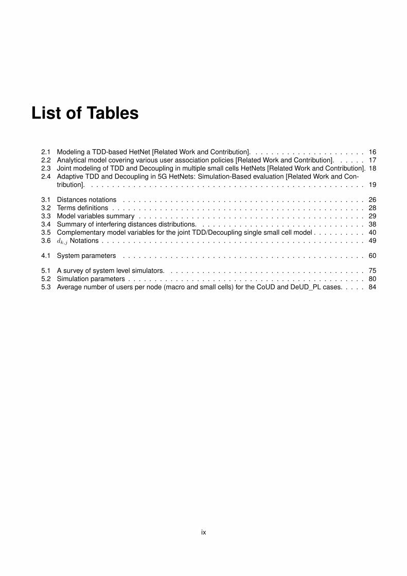
List of Tables
2.1 Modeling a TDD-based HetNet [Related Work and Contribution]. . . . . . . . . . . . . . . . . . . . . . 162.2 Analytical model covering various user association policies [Related Work and Contribution]. . . . . . 172.3 Joint modeling of TDD and Decoupling in multiple small cells HetNets [Related Work and Contribution]. 182.4 Adaptive TDD and Decoupling in 5G HetNets: Simulation-Based evaluation [Related Work and Con-
tribution]. . . . . . . . . . . . . . . . . . . . . . . . . . . . . . . . . . . . . . . . . . . . . . . . . . . . . 19
3.1 Distances notations . . . . . . . . . . . . . . . . . . . . . . . . . . . . . . . . . . . . . . . . . . . . . . 263.2 Terms definitions . . . . . . . . . . . . . . . . . . . . . . . . . . . . . . . . . . . . . . . . . . . . . . . . 283.3 Model variables summary . . . . . . . . . . . . . . . . . . . . . . . . . . . . . . . . . . . . . . . . . . . 293.4 Summary of interfering distances distributions. . . . . . . . . . . . . . . . . . . . . . . . . . . . . . . . 383.5 Complementary model variables for the joint TDD/Decoupling single small cell model . . . . . . . . . . 403.6 dk,j Notations . . . . . . . . . . . . . . . . . . . . . . . . . . . . . . . . . . . . . . . . . . . . . . . . . . 49
4.1 System parameters . . . . . . . . . . . . . . . . . . . . . . . . . . . . . . . . . . . . . . . . . . . . . . 60
5.1 A survey of system level simulators. . . . . . . . . . . . . . . . . . . . . . . . . . . . . . . . . . . . . . 755.2 Simulation parameters . . . . . . . . . . . . . . . . . . . . . . . . . . . . . . . . . . . . . . . . . . . . . 805.3 Average number of users per node (macro and small cells) for the CoUD and DeUD_PL cases. . . . . 84
ix

List of Figures
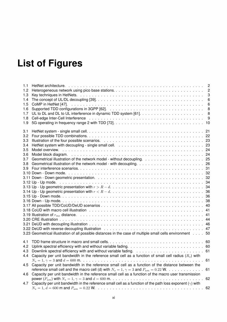
1.1 HetNet architecture. . . . . . . . . . . . . . . . . . . . . . . . . . . . . . . . . . . . . . . . . . . . . . . 21.2 Heterogeneous network using pico base stations. . . . . . . . . . . . . . . . . . . . . . . . . . . . . . . 21.3 Key techniques in HetNets. . . . . . . . . . . . . . . . . . . . . . . . . . . . . . . . . . . . . . . . . . . 31.4 The concept of UL/DL decoupling [39]. . . . . . . . . . . . . . . . . . . . . . . . . . . . . . . . . . . . . 61.5 CoMP in HetNet [47]. . . . . . . . . . . . . . . . . . . . . . . . . . . . . . . . . . . . . . . . . . . . . . 61.6 Supported TDD configurations in 3GPP [62]. . . . . . . . . . . . . . . . . . . . . . . . . . . . . . . . . 81.7 UL to DL and DL to UL interference in dynamic TDD system [61]. . . . . . . . . . . . . . . . . . . . . . 81.8 Cell-edge Inter-Cell Interference . . . . . . . . . . . . . . . . . . . . . . . . . . . . . . . . . . . . . . . 91.9 5G operating in frequency range 2 with TDD [72]. . . . . . . . . . . . . . . . . . . . . . . . . . . . . . . 10
3.1 HetNet system - single small cell. . . . . . . . . . . . . . . . . . . . . . . . . . . . . . . . . . . . . . . . 213.2 Four possible TDD combinations. . . . . . . . . . . . . . . . . . . . . . . . . . . . . . . . . . . . . . . . 223.3 Illustration of the four possible scenarios. . . . . . . . . . . . . . . . . . . . . . . . . . . . . . . . . . . 233.4 HetNet system with decoupling - single small cell. . . . . . . . . . . . . . . . . . . . . . . . . . . . . . 233.5 Model overview. . . . . . . . . . . . . . . . . . . . . . . . . . . . . . . . . . . . . . . . . . . . . . . . . 243.6 Model block diagram. . . . . . . . . . . . . . . . . . . . . . . . . . . . . . . . . . . . . . . . . . . . . . 243.7 Geometrical illustration of the network model - without decoupling. . . . . . . . . . . . . . . . . . . . . 253.8 Geometrical illustration of the network model - with decoupling. . . . . . . . . . . . . . . . . . . . . . . 263.9 Four interference scenarios. . . . . . . . . . . . . . . . . . . . . . . . . . . . . . . . . . . . . . . . . . . 313.10 Down - Down mode. . . . . . . . . . . . . . . . . . . . . . . . . . . . . . . . . . . . . . . . . . . . . . . 323.11 Down - Down geometric presentation. . . . . . . . . . . . . . . . . . . . . . . . . . . . . . . . . . . . . 323.12 Up - Up mode. . . . . . . . . . . . . . . . . . . . . . . . . . . . . . . . . . . . . . . . . . . . . . . . . . 343.13 Up - Up geometric presentation with r > R− d. . . . . . . . . . . . . . . . . . . . . . . . . . . . . . . . 343.14 Up - Up geometric presentation with r < R− d. . . . . . . . . . . . . . . . . . . . . . . . . . . . . . . . 363.15 Up - Down mode. . . . . . . . . . . . . . . . . . . . . . . . . . . . . . . . . . . . . . . . . . . . . . . . . 363.16 Down - Up mode. . . . . . . . . . . . . . . . . . . . . . . . . . . . . . . . . . . . . . . . . . . . . . . . . 383.17 All possible TDD/CoUD/DeUD scenarios . . . . . . . . . . . . . . . . . . . . . . . . . . . . . . . . . . . 403.18 CoUD with macro cell illustration . . . . . . . . . . . . . . . . . . . . . . . . . . . . . . . . . . . . . . . 413.19 Illustration of rme distance. . . . . . . . . . . . . . . . . . . . . . . . . . . . . . . . . . . . . . . . . . . 413.20 CRE illustration . . . . . . . . . . . . . . . . . . . . . . . . . . . . . . . . . . . . . . . . . . . . . . . . . 443.21 DeUD with decoupling illustration . . . . . . . . . . . . . . . . . . . . . . . . . . . . . . . . . . . . . . . 463.22 DeUD with reverse decoupling illustration . . . . . . . . . . . . . . . . . . . . . . . . . . . . . . . . . . 473.23 Geometrical illustration of all possible distances in the case of multiple small cells environment . . . . 50
4.1 TDD frame structure in macro and small cells. . . . . . . . . . . . . . . . . . . . . . . . . . . . . . . . . 604.2 Uplink spectral efficiency with and without variable fading. . . . . . . . . . . . . . . . . . . . . . . . . . 604.3 Downlink spectral efficiency with and without variable fading. . . . . . . . . . . . . . . . . . . . . . . . 614.4 Capacity per unit bandwidth in the reference small cell as a function of small cell radius (Rs) with
Ns = 1, γ = 3 and d = 600 m. . . . . . . . . . . . . . . . . . . . . . . . . . . . . . . . . . . . . . . . . . 614.5 Capacity per unit bandwidth in the reference small cell as a function of the distance between the
reference small cell and the macro cell (d) with Ns = 1, γ = 3 and Pum = 0.22 W. . . . . . . . . . . . . 614.6 Capacity per unit bandwidth in the reference small cell as a function of the macro user transmission
power (Pum) with Ns = 1, γ = 3 and d = 600 m. . . . . . . . . . . . . . . . . . . . . . . . . . . . . . . . 624.7 Capacity per unit bandwidth in the reference small cell as a function of the path loss exponent (γ) with
Ns = 1, d = 600 m and Pum = 0.22 W. . . . . . . . . . . . . . . . . . . . . . . . . . . . . . . . . . . . . 62
xi
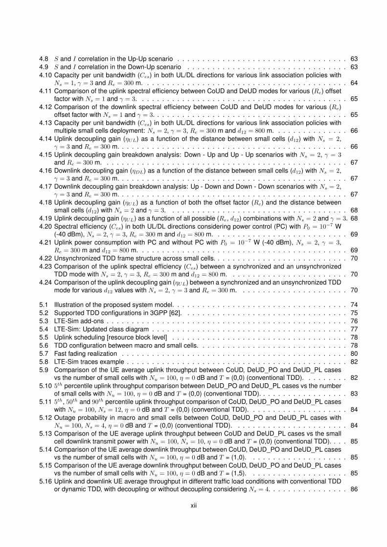
4.8 S and I correlation in the Up-Up scenario . . . . . . . . . . . . . . . . . . . . . . . . . . . . . . . . . . 634.9 S and I correlation in the Down-Up scenario . . . . . . . . . . . . . . . . . . . . . . . . . . . . . . . . 634.10 Capacity per unit bandwidth (Ces) in both UL/DL directions for various link association policies with
Ns = 1, γ = 3 and Re = 300 m. . . . . . . . . . . . . . . . . . . . . . . . . . . . . . . . . . . . . . . . . 644.11 Comparison of the uplink spectral efficiency between CoUD and DeUD modes for various (Re) offset
factor with Ns = 1 and γ = 3. . . . . . . . . . . . . . . . . . . . . . . . . . . . . . . . . . . . . . . . . . 654.12 Comparison of the downlink spectral efficiency between CoUD and DeUD modes for various (Re)
offset factor with Ns = 1 and γ = 3. . . . . . . . . . . . . . . . . . . . . . . . . . . . . . . . . . . . . . . 654.13 Capacity per unit bandwidth (Ces) in both UL/DL directions for various link association policies with
multiple small cells deployment: Ns = 2, γ = 3, Re = 300 m and d12 = 800 m. . . . . . . . . . . . . . . 664.14 Uplink decoupling gain (ηUL) as a function of the distance between small cells (d12) with Ns = 2,
γ = 3 and Re = 300 m. . . . . . . . . . . . . . . . . . . . . . . . . . . . . . . . . . . . . . . . . . . . . . 664.15 Uplink decoupling gain breakdown analysis: Down - Up and Up - Up scenarios with Ns = 2, γ = 3
and Re = 300 m. . . . . . . . . . . . . . . . . . . . . . . . . . . . . . . . . . . . . . . . . . . . . . . . . 674.16 Downlink decoupling gain (ηDL) as a function of the distance between small cells (d12) with Ns = 2,
γ = 3 and Re = 300 m. . . . . . . . . . . . . . . . . . . . . . . . . . . . . . . . . . . . . . . . . . . . . . 674.17 Downlink decoupling gain breakdown analysis: Up - Down and Down - Down scenarios with Ns = 2,
γ = 3 and Re = 300 m. . . . . . . . . . . . . . . . . . . . . . . . . . . . . . . . . . . . . . . . . . . . . . 674.18 Uplink decoupling gain (ηUL) as a function of both the offset factor (Re) and the distance between
small cells (d12) with Ns = 2 and γ = 3. . . . . . . . . . . . . . . . . . . . . . . . . . . . . . . . . . . . 684.19 Uplink decoupling gain (ηUL) as a function of all possible (Re, d12) combinations with Ns = 2 and γ = 3. 684.20 Spectral efficiency (Ces) in both UL/DL directions considering power control (PC) with P0 = 10−7 W
(-40 dBm), Ns = 2, γ = 3, Re = 300 m and d12 = 800 m. . . . . . . . . . . . . . . . . . . . . . . . . . . 694.21 Uplink power consumption with PC and without PC with P0 = 10−7 W (-40 dBm), Ns = 2, γ = 3,
Re = 300 m and d12 = 800 m. . . . . . . . . . . . . . . . . . . . . . . . . . . . . . . . . . . . . . . . . . 694.22 Unsynchronized TDD frame structure across small cells. . . . . . . . . . . . . . . . . . . . . . . . . . . 704.23 Comparison of the uplink spectral efficiency (Ces) between a synchronized and an unsynchronized
TDD mode with Ns = 2, γ = 3, Re = 300 m and d12 = 800 m. . . . . . . . . . . . . . . . . . . . . . . . 704.24 Comparison of the uplink decoupling gain (ηUL) between a synchronized and an unsynchronized TDD
mode for various d12 values with Ns = 2, γ = 3 and Re = 300 m. . . . . . . . . . . . . . . . . . . . . . 70
5.1 Illustration of the proposed system model. . . . . . . . . . . . . . . . . . . . . . . . . . . . . . . . . . . 745.2 Supported TDD configurations in 3GPP [62]. . . . . . . . . . . . . . . . . . . . . . . . . . . . . . . . . 755.3 LTE-Sim add-ons . . . . . . . . . . . . . . . . . . . . . . . . . . . . . . . . . . . . . . . . . . . . . . . . 765.4 LTE-Sim: Updated class diagram . . . . . . . . . . . . . . . . . . . . . . . . . . . . . . . . . . . . . . . 775.5 Uplink scheduling [resource block level] . . . . . . . . . . . . . . . . . . . . . . . . . . . . . . . . . . . 785.6 TDD configuration between macro and small cells. . . . . . . . . . . . . . . . . . . . . . . . . . . . . . 785.7 Fast fading realization . . . . . . . . . . . . . . . . . . . . . . . . . . . . . . . . . . . . . . . . . . . . . 805.8 LTE-Sim traces example . . . . . . . . . . . . . . . . . . . . . . . . . . . . . . . . . . . . . . . . . . . . 825.9 Comparison of the UE average uplink throughput between CoUD, DeUD_PO and DeUD_PL cases
vs the number of small cells with Nu = 100, η = 0 dB and T = (0,0) (conventional TDD). . . . . . . . . 825.10 5th percentile uplink throughput comparison between DeUD_PO and DeUD_PL cases vs the number
of small cells with Nu = 100, η = 0 dB and T = (0,0) (conventional TDD). . . . . . . . . . . . . . . . . . 835.11 5th, 50th and 90th percentile uplink throughput comparison of CoUD, DeUD_PO and DeUD_PL cases
with Nu = 100, Ns = 12, η = 0 dB and T = (0,0) (conventional TDD). . . . . . . . . . . . . . . . . . . . 845.12 Outage probability in macro and small cells between CoUD, DeUD_PO and DeUD_PL cases with
Nu = 100, Ns = 4, η = 0 dB and T = (0,0) (conventional TDD). . . . . . . . . . . . . . . . . . . . . . . 845.13 Comparison of the UE average uplink throughput between CoUD and DeUD_PL cases vs the small
cell downlink transmit power with Nu = 100, Ns = 10, η = 0 dB and T = (0,0) (conventional TDD). . . . 855.14 Comparison of the UE average downlink throughput between CoUD, DeUD_PO and DeUD_PL cases
vs the number of small cells with Nu = 100, η = 0 dB and T = (1,0). . . . . . . . . . . . . . . . . . . . 855.15 Comparison of the UE average downlink throughput between CoUD, DeUD_PO and DeUD_PL cases
vs the number of small cells with Nu = 100, η = 0 dB and T = (1,5). . . . . . . . . . . . . . . . . . . . 855.16 Uplink and downlink UE average throughput in different traffic load conditions with conventional TDD
or dynamic TDD, with decoupling or without decoupling considering Ns = 4. . . . . . . . . . . . . . . . 86
xii
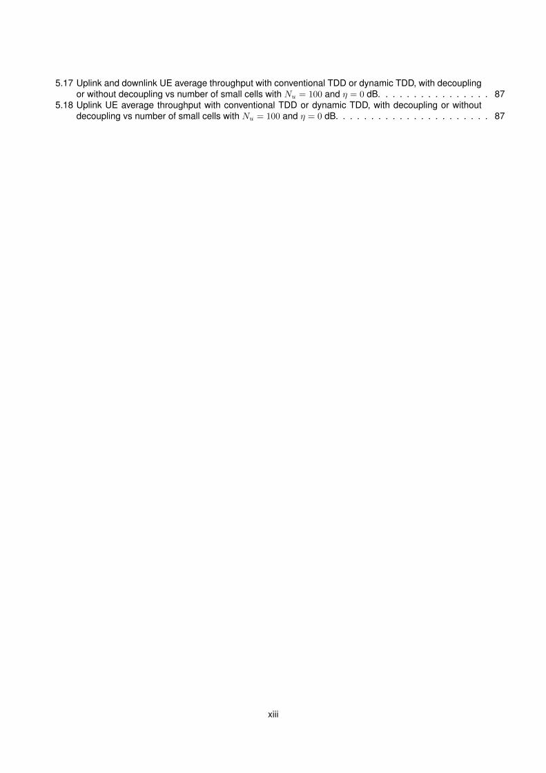
5.17 Uplink and downlink UE average throughput with conventional TDD or dynamic TDD, with decouplingor without decoupling vs number of small cells with Nu = 100 and η = 0 dB. . . . . . . . . . . . . . . . 87
5.18 Uplink UE average throughput with conventional TDD or dynamic TDD, with decoupling or withoutdecoupling vs number of small cells with Nu = 100 and η = 0 dB. . . . . . . . . . . . . . . . . . . . . . 87
xiii

Chapter 1
Introduction
In this chapter, we first describe the challenges faced in mobile networks nowadays and the way to address them.Second, we present the key techniques in next generation HetNets compared to classical HetNets. Further, the mo-tivation behind adopting dynamic TDD and decoupling techniques in next generation 5G HetNets is also presented.Finally, we explain the goals and research objectives of this study.
1.1 Challenges in Mobile Networks
Over the past few years, the demand for mobile traffic has been largely increasing. According to [1], the globalmobile data will reach 77 exabytes per month by 2022. Recent reports show that more than 600 million (i.e, 648million) mobile devices were added in 2017. By 2022, there will be 8.4 billion personal mobile-ready devices, and3.9 billion Machine-to-Machine (M2M) connections.In response to this growth, mobile operators resort to flexible and efficient solutions to cope with the continuousdemand on traffic. They have recently adopted HetNet solutions to offload traffic from a macro base station (BS)to a small cell BS, in the aim of improving the overall system performance. Yet, because of the load traffic disparityin DL and UL, it becomes essential to dynamically adjust UL/DL resources. In particular, the rapid growth in videostreaming traffic results in asymmetric and dynamically changing UL and DL traffic loads. To support this newapproach, dynamic time-division duplexing (TDD) ( [2], [3]) has been proposed. Nevertheless, the importance ofUL arises along with the evolution of social networking and cloud solutions. Therefore, it is of great interest tointroduce novel techniques that mitigate UL interferences, improve UL and DL throughputs and allow as well, abetter use of radio resources by providing adequate load balancing among UL and DL. Such an additional featureis the decoupled UL/DL access ( [4], [5]).Consequently and in order to address the aforementioned challenges, an important shift from classical HetNets tonext-generation HetNets (5G) is emerging in the aim of improving overall system performance.
1.2 Heterogeneous Networks (HetNets)
The heterogeneous networks [6] approach consists in complementing the macro layer with low power nodes suchas small cell base stations. This approach has been considered a way to improve the capacity and data rate inthe areas covered by these low power nodes; they are mostly distributed depending on the areas that generatehigher traffic. HetNets involve the use of different types of radio technology and employ low power nodes workingtogether with the current macro cells; that is to say, they may coexist in the same geographical area sharing thesame spectrum, so it is not necessary that they provide full area coverage. For this reason, while the location of themacro stations is generally carefully planned, the low power nodes are typically deployed in a relatively unplannedmanner. Usually, the main aim of low power nodes is to eliminate coverage holes in the macro network, improvecapacity in hotspots and improve cell edge throughput; that is why, the location chosen for their deployment is basedon the knowledge of coverage issues and traffic density in the network.Deploying low power nodes can be challenging, as performance depends on close proximity to where traffic isgenerated and, due to their reduced coverage range, a lot of them may be needed. Nevertheless, owing to theirlower transmit power and smaller physical size, low power stations can offer flexible site acquisitions. Furthermore,
1
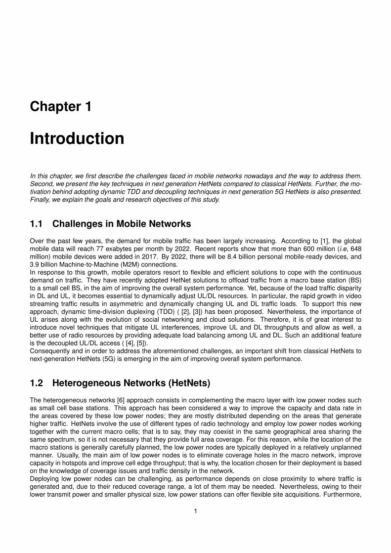
HetNets allow improving spectral efficiency per unit area and offer very high capacity and data rates in areas coveredby the low power nodes. Therefore, it is an attractive solution in scenarios where users are highly clustered.
Figure 1.1: HetNet architecture.
1.2.1 HetNets Motivation
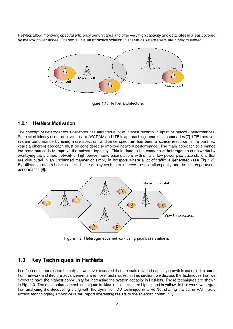
The concept of heterogeneous networks has attracted a lot of interest recently to optimize network performances.Spectral efficiency of current systems like WCDMA and LTE is approaching theoretical boundaries [7], LTE improvessystem performance by using more spectrum and since spectrum has been a scarce resource in the past fewyears a different approach must be considered to improve network performance. The main approach to enhancethe performance is to improve the network topology. This is done in the scenario of heterogeneous networks byoverlaying the planned network of high power macro base stations with smaller low power pico base stations thatare distributed in an unplanned manner or simply in hotspots where a lot of traffic is generated (see Fig 1.2).By offloading macro base stations, these deployments can improve the overall capacity and the cell edge users’performance [8].
Figure 1.2: Heterogeneous network using pico base stations.
1.3 Key Techniques in HetNets
In reference to our research analysis, we have observed that the main driver of capacity growth is expected to comefrom network architecture advancements and novel techniques. In this section, we discuss the techniques that weexpect to have the highest opportunity for increasing the system capacity in HetNets. These techniques are shownin Fig. 1.3. The main enhancement techniques tackled in this thesis are highlighted in yellow. In this work, we arguethat analyzing the decoupling along with the dynamic TDD technique in a HetNet sharing the same RAT (radioaccess technologies) among cells, will report interesting results to the scientific community.
2
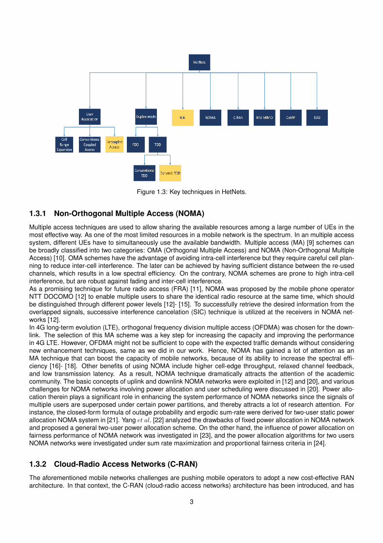
Figure 1.3: Key techniques in HetNets.
1.3.1 Non-Orthogonal Multiple Access (NOMA)
Multiple access techniques are used to allow sharing the available resources among a large number of UEs in themost effective way. As one of the most limited resources in a mobile network is the spectrum. In an multiple accesssystem, different UEs have to simultaneously use the available bandwidth. Multiple access (MA) [9] schemes canbe broadly classified into two categories: OMA (Orthogonal Multiple Access) and NOMA (Non-Orthogonal MultipleAccess) [10]. OMA schemes have the advantage of avoiding intra-cell interference but they require careful cell plan-ning to reduce inter-cell interference. The later can be achieved by having sufficient distance between the re-usedchannels, which results in a low spectral efficiency. On the contrary, NOMA schemes are prone to high intra-cellinterference, but are robust against fading and inter-cell interference.As a promising technique for future radio access (FRA) [11], NOMA was proposed by the mobile phone operatorNTT DOCOMO [12] to enable multiple users to share the identical radio resource at the same time, which shouldbe distinguished through different power levels [12]- [15]. To successfully retrieve the desired information from theoverlapped signals, successive interference cancelation (SIC) technique is utilized at the receivers in NOMA net-works [12].In 4G long-term evolution (LTE), orthogonal frequency division multiple access (OFDMA) was chosen for the down-link. The selection of this MA scheme was a key step for increasing the capacity and improving the performancein 4G LTE. However, OFDMA might not be sufficient to cope with the expected traffic demands without consideringnew enhancement techniques, same as we did in our work. Hence, NOMA has gained a lot of attention as anMA technique that can boost the capacity of mobile networks, because of its ability to increase the spectral effi-ciency [16]- [18]. Other benefits of using NOMA include higher cell-edge throughput, relaxed channel feedback,and low transmission latency. As a result, NOMA technique dramatically attracts the attention of the academiccommunity. The basic concepts of uplink and downlink NOMA networks were exploited in [12] and [20], and variouschallenges for NOMA networks involving power allocation and user scheduling were discussed in [20]. Power allo-cation therein plays a significant role in enhancing the system performance of NOMA networks since the signals ofmultiple users are superposed under certain power partitions, and thereby attracts a lot of research attention. Forinstance, the closed-form formula of outage probability and ergodic sum-rate were derived for two-user static powerallocation NOMA system in [21]. Yang et al. [22] analyzed the drawbacks of fixed power allocation in NOMA networkand proposed a general two-user power allocation scheme. On the other hand, the influence of power allocation onfairness performance of NOMA network was investigated in [23], and the power allocation algorithms for two usersNOMA networks were investigated under sum rate maximization and proportional fairness criteria in [24].
1.3.2 Cloud-Radio Access Networks (C-RAN)
The aforementioned mobile networks challenges are pushing mobile operators to adopt a new cost-effective RANarchitecture. In that context, the C-RAN (cloud-radio access networks) architecture has been introduced, and has
3
been motivated in many projects, such as the “Interworking and Joint Design of an Open Access and BackhaulNetwork Architecture for Small Cells based on Cloud Networks” [25], launched in 2012 by the European Commis-sion, and the “Mobile Cloud Networking (MCN)” [26], launched in 2013 also by the European Commission. Further,many Asian-Pacific MNOs have been tempted by the advantages of C-RAN architecture, and have already startedto plan its deployment. For example, Korean SK Telecom and NTT-DoCoMO have announced early trials of C-RANin 2019. The C-RAN consists of a new cloud architecture, aiming to face the need of TCOs reduction. This approachwas conceived from the cloud computing concept. In C-RAN, BBUs (Baseband Units) are migrated from sites, tobe gathered in a single location. The latter consists of a central office or a super macro site used to aggregateBBUs. RRHs (Remote Radio Heads) are connected to BBUs through high-bandwidth and low latency optical links.Precisely, baseband elements are employed efficiently and follow the instantaneous load conditions in the network,instead of adopting the maximum traffic of individual base stations. Consequently, processing power is reduced andadapts to network instantaneous load.
1.3.3 Multi-User MIMO (MU-MIMO)
Multiple antenna technology, known as MIMO, is playing an important role in 4G cellular networks, and is expectedto be even more essential for meeting 5G target data rates [28]. One key such technique is multiuser MIMO (MU-MIMO), which allows a base station (BS) with many antennas to communicate simultaneously with numerous mobileunits each with a very small number of antennas. Although multiuser MIMO also known as space division multipleaccess (SDMA) has been known for quite some time and previous implementation efforts have been relatively disap-pointing, enthusiasm has been recently renewed, as seen in the extensive recent literature on “massive MIMO” [29],as well as the very recent 3GPP standardization of full-dimension (FD) MIMO, which can support 64 antennas in a2D array at the BS to communicate simultaneously with 32 mobile terminals [30].Multi-antenna transmissions bring significant additional complexity to HetNet analysis, primarily due to the complex-ity of the random matrix channel. As shown in [31], the invariance property may be lost in multi-antenna HetNets,i.e., the outage probability will increase as the BS density increases. This is mainly because the distributions ofboth the signal and interference depend on the number of BS antennas and the adopted multi-antenna transmissionstrategy of each BS. The work [31] relied on stochastic ordering to compare different multi-antenna techniques, butsuch a method cannot be used for quantitative analysis, since the SINR and SIR distributions were not provided.That work was extended to incorporate load balancing and thus the achievable rate in [32]. Other notable efforts onMIMO HetNets include work limited to two tiers [33], [34], and the analysis in [35], which focused on the interferencedistribution.
1.3.4 User association
Conventional Coupled Access
In classical HetNets, conventional coupled UL/DL access mode is adopted, where each user is associated in down-link and uplink with a single cell. Cell association criteria in DL and UL is based on DL Reference Signal ReceivedPower (RSRP) which is the conventional LTE user association policy. That is to say, each UE selects its serving cellID according to the cell from which the largest RSRP is provided :
CellIDserving = argmaxi(RSRPi).
Cell Range Expansion (CRE)
Cell selection in LTE is based on terminal measurements of the received power of the downlink signal or morespecifically the cell specific reference (CRS) downlink signaling. However, in a heterogeneous network, there aredifferent types of base stations with different transmission powers including different powers of CRS. This approachfor cell selection would be unfair to the low power nodes (pico-eNBs), as most probably the terminal will choosethe higher power base stations (macro-eNBs), even if the path loss to the pico-eNB is smaller and this will not beoptimal in terms of:
1. Uplink coverage: As the terminal has a lower path loss to the pico-eNB but instead it will select the macro-eNB.
4
2. Downlink capacity: Pico-eNBs will be under-utilized as fewer users are connected to them while the macro-eNBs could be overloaded even if macro-eNBs and pico-eNBs are using the same resources in terms ofspectrum, so the cell-splitting, also the offload gain is not large and the resources are not well utilized.
3. Interference: Due to the high transmission power of the macro-eNBs, then the Macro-eNB transmission isassociated with a high interference to the pico-eNB users which denies them to use the same physical re-sources.
As a solution for the first two points, cell selection could be dependent on estimates of the uplink path loss, whichin practice can be done by applying a cell-specific offset to the received power measurements used in typical cellselection. This offset would somehow compensate for the transmitting power differences between the macro-eNBsand pico-eNBs; it would also extend the coverage area of the Pico-eNB, or in other words extend the area wherethe pico-eNB is selected. This area is called "Range Expansion” [36].In this technique, users are offloaded to smaller cells using an association bias or offset. Formally, if there are Kcandidate tiers available for a user to associate, then the index of the chosen tier is:
k∗ = argmaxi=1−>kBiPrx,i, (1.1)
where Bi is the bias for tier i and Prx,i is the received power from tier i. By convention, tier 1 is the macro cell tierand has a bias of 1 (0 dB). For example a small cell bias of 10 dB means a UE would associate with the small cellup until its received power was more than 10 dB less than the macro cell base station.However, the difference in transmission powers of the macro-eNBs and the pico-eNB in the range expansion area,makes the users in the range expansion area more prone to interference from the macro-eNB. So along with thebenefits of range expansion, comes the disadvantage of the high inter-cell interference that the macro layer imposeson the users in the range expansion area of the pico layer.
UL/DL Decoupled Access
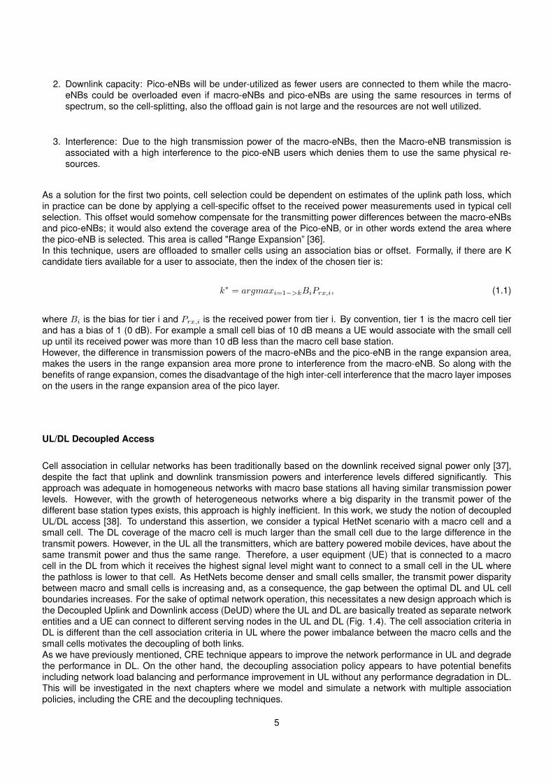
Cell association in cellular networks has been traditionally based on the downlink received signal power only [37],despite the fact that uplink and downlink transmission powers and interference levels differed significantly. Thisapproach was adequate in homogeneous networks with macro base stations all having similar transmission powerlevels. However, with the growth of heterogeneous networks where a big disparity in the transmit power of thedifferent base station types exists, this approach is highly inefficient. In this work, we study the notion of decoupledUL/DL access [38]. To understand this assertion, we consider a typical HetNet scenario with a macro cell and asmall cell. The DL coverage of the macro cell is much larger than the small cell due to the large difference in thetransmit powers. However, in the UL all the transmitters, which are battery powered mobile devices, have about thesame transmit power and thus the same range. Therefore, a user equipment (UE) that is connected to a macrocell in the DL from which it receives the highest signal level might want to connect to a small cell in the UL wherethe pathloss is lower to that cell. As HetNets become denser and small cells smaller, the transmit power disparitybetween macro and small cells is increasing and, as a consequence, the gap between the optimal DL and UL cellboundaries increases. For the sake of optimal network operation, this necessitates a new design approach which isthe Decoupled Uplink and Downlink access (DeUD) where the UL and DL are basically treated as separate networkentities and a UE can connect to different serving nodes in the UL and DL (Fig. 1.4). The cell association criteria inDL is different than the cell association criteria in UL where the power imbalance between the macro cells and thesmall cells motivates the decoupling of both links.As we have previously mentioned, CRE technique appears to improve the network performance in UL and degradethe performance in DL. On the other hand, the decoupling association policy appears to have potential benefitsincluding network load balancing and performance improvement in UL without any performance degradation in DL.This will be investigated in the next chapters where we model and simulate a network with multiple associationpolicies, including the CRE and the decoupling techniques.
5
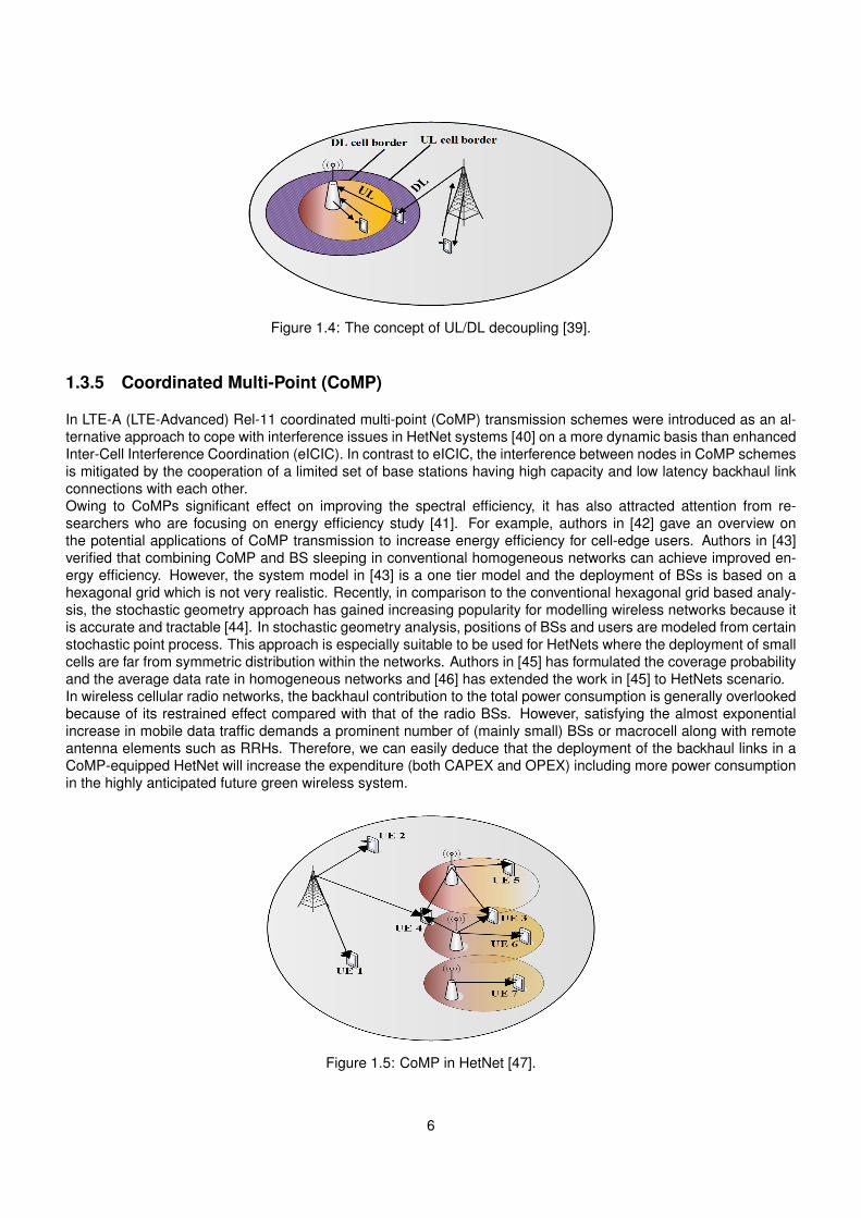
Figure 1.4: The concept of UL/DL decoupling [39].
1.3.5 Coordinated Multi-Point (CoMP)
In LTE-A (LTE-Advanced) Rel-11 coordinated multi-point (CoMP) transmission schemes were introduced as an al-ternative approach to cope with interference issues in HetNet systems [40] on a more dynamic basis than enhancedInter-Cell Interference Coordination (eICIC). In contrast to eICIC, the interference between nodes in CoMP schemesis mitigated by the cooperation of a limited set of base stations having high capacity and low latency backhaul linkconnections with each other.Owing to CoMPs significant effect on improving the spectral efficiency, it has also attracted attention from re-searchers who are focusing on energy efficiency study [41]. For example, authors in [42] gave an overview onthe potential applications of CoMP transmission to increase energy efficiency for cell-edge users. Authors in [43]verified that combining CoMP and BS sleeping in conventional homogeneous networks can achieve improved en-ergy efficiency. However, the system model in [43] is a one tier model and the deployment of BSs is based on ahexagonal grid which is not very realistic. Recently, in comparison to the conventional hexagonal grid based analy-sis, the stochastic geometry approach has gained increasing popularity for modelling wireless networks because itis accurate and tractable [44]. In stochastic geometry analysis, positions of BSs and users are modeled from certainstochastic point process. This approach is especially suitable to be used for HetNets where the deployment of smallcells are far from symmetric distribution within the networks. Authors in [45] has formulated the coverage probabilityand the average data rate in homogeneous networks and [46] has extended the work in [45] to HetNets scenario.In wireless cellular radio networks, the backhaul contribution to the total power consumption is generally overlookedbecause of its restrained effect compared with that of the radio BSs. However, satisfying the almost exponentialincrease in mobile data traffic demands a prominent number of (mainly small) BSs or macrocell along with remoteantenna elements such as RRHs. Therefore, we can easily deduce that the deployment of the backhaul links in aCoMP-equipped HetNet will increase the expenditure (both CAPEX and OPEX) including more power consumptionin the highly anticipated future green wireless system.
Figure 1.5: CoMP in HetNet [47].
6
1.3.6 UL/DL Decoupling and CoMP
Coordinated Multi-Point (CoMP) transmission or reception, has gained popularity in the context of HetNets as ameans to increase the UE achievable throughput. eNBs within the same cluster communicate via backhaul links(i.e., via the X2 interface) with the objective of minimizing the inter-cell interference and capitalize on the benefitsof distributed antenna systems. In fact, interference within a cooperation cluster can be effectively cancelled [48],[51]. This level of coordination and cooperation can be carried out in both UL and DL, and the realization of suchcoordination relies strongly on the availability of sufficient backhaul capacity, first to serve the UE in the cell cluster,and second to communicate with other cells in the cooperation cluster. This backhaul dependency can be verylimiting in situations of high load, and in capacity limited links. The increased flexibility provided by decoupled ULand DL associations provides advantages when selecting UL and DL coordinated transmissions or receptions. Inparticular, there is no need to have both UL and DL simultaneous connection to the entire cooperating set of basestations and the UE could have unequal UL and DL active links (as in the case of CA). This flexible associationinside the cluster, and the interoperability of DeUD with CoMP goes one step further in the device-centric network,since the UE can select independently the number and position of DL and UL serving cells, according to severalinput parameters, as backhaul capacity, power limitation, throughput maximization, among others
1.3.7 UL/DL Decoupling Enabler between CoMP and C-RAN
Implementing a decoupled cell association in a real network requires excellent connectivity and modest cooperationbetween different base stations. The main requirement DeUD imposes is a low latency connection between thedownlink and the uplink base stations, to allow a fast exchange of control messages [52]. We emphasise thatdifferently from the most sophisticated forms of CoMP (e.g. joint processing) where a high throughput backhaulconnection between BSs is required to allow rapid data exchange, DeUD does not impose a tight requirement onthe backhaul capacity. Put another way, DeUD allows gains similar to uplink joint processing (about 100% edgeand average throughput gain), but with lower deployment costs. Compared to using MIMO or new spectrum toincrease the throughput, the cost comparison is even more favorable to DeUD. The ongoing trend towards usingpartial or full Radio Access Network (RAN) centralization in deployments where a high-speed backhaul is available,will be an enabler for downlink and uplink decoupling, as signalling will be routed to a central processing unit withlow-latency connections. In particular, partial centralization refers to those local deployments (e.g. indoor) wherethe transmission points serving the same local area are all connected to the same baseband processing central unit.Full centralization, often referred as Cloud-RAN, extends this approach to larger areas, where a large number of RFunits are connected to the same baseband processing central unit. Given this already ongoing trend towards morecentralized RAN architectures, which are underpinned by low-latency connectivity between BSs, the incrementalcost of DeUD appears negligible in such scenarios.
1.3.8 Device to Device (D2D) Communications
With the spectral performance of the wireless link approaching the theoretical limits due to present cellular wirelessnetworks, researchers have been working on various aspects in the framework of LTE-Advanced to further facilitatethe mobile users in a ubiquitous and cost effective manner [53]. One of the ways of increasing the achievable rate incellular communications is direct communication between closely located mobile users. This form of communicationis referred to as device-to-device (D2D) communication [ [55], [56]]. D2D communication, is a technique that is firstintroduced in 3GPP Release 12 and 13 [54]. Mobile devices involved in D2D communication form a direct linkwith each other, without the need of routing traffic via the cellular access network, resulting in lower transmit powerand end-to-end delay, as well as freeing network resources. The lower transmit powers manifest through reducedinterference levels in the system and battery power savings, while the improved rate is achieved as a result of lowpath-loss between any pair of devices involved in D2D communication [57]. The concept of D2D was presented inseveral studies as a promising solution to increase network capacity [58]. In this concept, the user can relay otheruser’s traffic to light loaded small cell using its resource [59] [60].
1.3.9 Dynamic TDD
In classical HetNets, either FDD or conventional TDD technique is adopted. Sharing the same static TDD configu-ration between macro cell from one side and the small cell from the other side, is what we refer to as conventionalTDD approach. However, the fifth-generation wireless communication systems (5G) are expected to support various
7
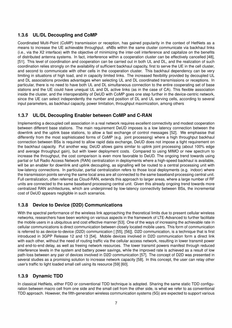
services, such as voice over IP (VoIP), online video, social networking, video sharing, etc. Due to the different uplinkand downlink traffic demand of these services, the asymmetric traffic is one remarkable characteristics of futuremobile communications. Besides, the instantaneous traffic condition of the network may vary significantly amongadjacent cells. To satisfy this asymmetric and dynamic traffic demand, dynamic TDD is one promising solution sincethe UL/DL transmission direction can be changed dynamically to adapt the instantaneous traffic variation [61]. Inthe 3GPP standard, dynamic TDD is supported by seven configurations with respect to different uplink and downlinktraffic ratios [62]. As shown in Fig. 1.6, each radio frame consists of 10 subframes, and the UL/DL ratio is different foreach TDD frame configuration. This enables either the macro cell or the small cells base stations to select differentconfigurations according to the traffic variation. As one special case of dynamic TDD, enhanced interference miti-
Figure 1.6: Supported TDD configurations in 3GPP [62].
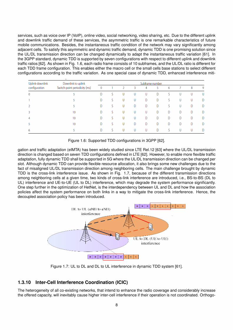
gation and traffic adaptation (eIMTA) has been widely studied since LTE Rel.12 [63] where the UL/DL transmissiondirection is changed based on seven TDD configurations defined in LTE [62]. However, to enable more flexible trafficadaptation, fully dynamic TDD shall be supported in 5G where the UL/DL transmission direction can be changed perslot. Although dynamic TDD can provide flexible resource allocation, it also brings some new challenges due to thefact of misaligned UL/DL transmission direction among neighboring cells. The main challenge brought by dynamicTDD is the cross-link interference issue. As shown in Fig. 1.7, because of the different transmission directionsamong neighboring cells at a given time, two kinds of cross-link interference are introduced, i.e., BS-to-BS (DL toUL) interference and UE-to-UE (UL to DL) interference, which may degrade the system performance significantly.One step further in the optimization of HetNet, is the interdependency between UL and DL and how the associationpolicies affect the system performance on both links in a way to mitigate the cross-link interference. Hence, thedecoupled association policy has been introduced.
Figure 1.7: UL to DL and DL to UL interference in dynamic TDD system [61].
1.3.10 Inter-Cell Interference Coordination (ICIC)
The heterogeneity of all co-existing networks, that intend to enhance the radio coverage and considerably increasethe offered capacity, will inevitably cause higher inter-cell interference if their operation is not coordinated. Orthogo-
8
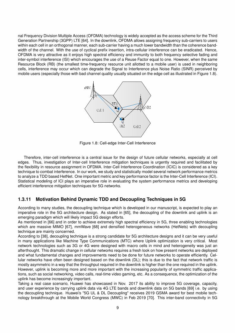
nal Frequency Division Multiple Access (OFDMA) technology is widely accepted as the access scheme for the ThirdGeneration Partnership (3GPP) LTE [64]. In the downlink, OFDMA allows assigning frequency sub-carriers to userswithin each cell in an orthogonal manner, each sub-carrier having a much lower bandwidth than the coherence band-width of the channel. With the use of cyclical prefix insertion, intra-cellular interference can be eradicated. Hence,OFDMA is very attractive as it enjoys high spectral efficiency and immunity to both frequency selective fading andinter-symbol interference (ISI) which encourages the use of a Reuse Factor equal to one. However, when the sameResource Block (RB) (the smallest time-frequency resource unit allotted to a mobile user) is used in neighboringcells, interference may occur which can degrade the Signal to Interference plus Noise Ratio (SINR) perceived bymobile users (especially those with bad channel quality usually situated on the edge cell as illustrated in Figure 1.8).
Figure 1.8: Cell-edge Inter-Cell Interference
Therefore, inter-cell interference is a central issue for the design of future cellular networks, especially at celledges. Thus, investigation of Inter-cell Interference mitigation techniques is urgently required and facilitated bythe flexibility in resource assignment in OFDMA. Inter-Cell Interference Coordination (ICIC) is considered as a keytechnique to combat interference. In our work, we study and statistically model several network performance metricsto analyze a TDD based HetNet. One important metric and key performance factor is the Inter-Cell Interference (ICI).Statistical modeling of ICI plays an imperative role in evaluating the system performance metrics and developingefficient interference mitigation techniques for 5G networks.
1.3.11 Motivation Behind Dynamic TDD and Decoupling Techniques in 5G
According to many studies, the decoupling technique which is developed in our manuscript, is expected to play animperative role in the 5G architecture design. As stated in [65], the decoupling of the downlink and uplink is anemerging paradigm which will likely impact 5G design efforts.As mentioned in [66] and in order to achieve extremely high spectral efficiency in 5G, three enabling technologieswhich are massive MIMO [67], mmWave [68] and densified heterogeneous networks (HetNets) with decouplingtechnique are mainly concerned.According to [38], decoupling technique is a strong candidate for 5G architecture designs and it can be very usefulin many applications like Machine Type Communications (MTC) where Uplink optimization is very critical. Mostnetwork technologies such as 3G or 4G were designed with macro cells in mind and heterogeneity was just anafterthought. This dramatic change in cellular networks requires a fresh look on how present networks are deployedand what fundamental changes and improvements need to be done for future networks to operate efficiently. Cel-lular networks have often been designed based on the downlink (DL); this is due to the fact that network traffic ismostly asymmetric in a way that the throughput required in the downlink is higher than the one required in the uplink.However, uplink is becoming more and more important with the increasing popularity of symmetric traffic applica-tions, such as social networking, video calls, real-time video gaming, etc. As a consequence, the optimization of theuplink has become increasingly important.Taking a real case scenario, Huawei has showcased in Nov. 2017 its ability to improve 5G coverage, capacity,and user experience by carrying uplink data via 4G LTE bands and downlink data on 5G bands [69] i.e. by usingthe decoupling technique. Huawei’s "5G UL & DL Decoupling" receives 2019 GSMA award for best mobile tech-nology breakthrough at the Mobile World Congress (MWC) in Feb 2019 [70]. This inter-band connectivity in 5G
9
networks [71] between two different radio technologies FR1 and FR2 has been clearly described in 3GPP Release16. As an example, a mobile user hosting a video streaming session which generally requires a high downlinkthroughput, will be associated in DL to a mmwave BS that offers a large bandwidth and thus a high throughput.However in UL, the mobile user suffering from a transmitted signal power limitation will be associated to a low fre-quency LTE BS to compensate and increase its uplink coverage.
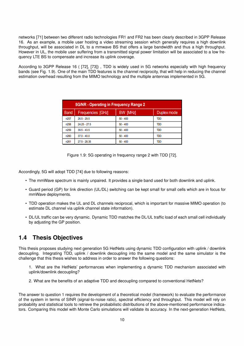
According to 3GPP Release 16 ( [72], [73]) , TDD is widely used in 5G networks especially with high frequencybands (see Fig. 1.9). One of the main TDD features is the channel reciprocity, that will help in reducing the channelestimation overhead resulting from the MIMO technology and the multiple antennas implemented in 5G.
Figure 1.9: 5G operating in frequency range 2 with TDD [72].
Accordingly, 5G will adopt TDD [74] due to following reasons:
• The mmWave spectrum is mainly unpaired. It provides a single band used for both downlink and uplink.
• Guard period (GP) for link direction (UL/DL) switching can be kept small for small cells which are in focus formmWave deployments.
• TDD operation makes the UL and DL channels reciprocal, which is important for massive MIMO operation (toestimate DL channel via uplink channel state information).
• DL/UL traffic can be very dynamic. Dynamic TDD matches the DL/UL traffic load of each small cell individuallyby adjusting the GP position.
1.4 Thesis Objectives
This thesis proposes studying next generation 5G HetNets using dynamic TDD configuration with uplink / downlinkdecoupling. Integrating TDD, uplink / downlink decoupling into the same model and the same simulator is thechallenge that this thesis wishes to address in order to answer the following questions:
1. What are the HetNets’ performances when implementing a dynamic TDD mechanism associated withuplink/downlink decoupling?
2. What are the benefits of an adaptive TDD and decoupling compared to conventional HetNets?
The answer to question 1 requires the development of a theoretical model (framework) to evaluate the performanceof the system in terms of SINR (signal-to-noise ratio), spectral efficiency and throughput. This model will rely onprobability and statistical tools to retrieve the probabilistic distributions of the above-mentioned performance indica-tors. Comparing this model with Monte Carlo simulations will validate its accuracy. In the next-generation HetNets,
10
deriving closed-form expressions for cross-tier/co-tier interference and user capacity in TDD HetNets helps in de-signing and optimizing advanced enhancement techniques, including but not limited to the decoupled access tech-nique. Deriving these expressions reduces as well the need for time consuming Monte-Carlo simulations, especiallyin the case of multiple small cells deployment where the time required to run Monte-Carlo simulations significantlyincreases.
The answer to question 2 requires the implementation of these techniques in a system level simulator allowingan adaptive TDD and uplink / downlink decoupling in a HetNet based system. The optimization of a HetNet basedsystem according to time-variant traffic loads with multiple small cells and multiple users, necessitates finding asystem level simulator where we can present the motivation and accurately assess the role of both decoupling anddynamic TDD techniques in the optimization problem. Our aim is to create appropriate simulation environment thatis relative to real scenarios i.e. simulations where multiple small cells are deployed in a heavy loaded HetNet systemand under various traffic loads. These simulations consider random users distribution with scheduling decisions inboth the uplink and the downlink directions. The gain provided by the proposed approaches will be evaluated basedon the simulation results.
11

Chapter 2
Related Work & Contributions
In this chapter, we review works that relate to our thesis and discuss in detail how our solution advances the stateof the art. In the comparison tables that follow, we indicate how the related articles contribute to each of the topicslisted in the table columns. This will clearly show how our works (highlighted in yellow) lift a number of scientificlocks addressed in the related articles.
2.1 Related Work
Modeling a TDD-based HetNet
Analyzing a TDD based HetNet requires modeling and studying several performance metrics. Interference modelingis considered a main metric in wireless communications as it plays a role in the design and analysis of wireless sys-tems and the establishment of advanced interference mitigation techniques. Interference models can also be helpfulin assessing the performance of a given network as a substitute to simulation-based approaches. The problem ofinterference modeling in small cell networks has been tackled recently using various tools and methods. Severalrecent studies considered the modeling of the Inter-Cell Interference (ICI), where closed-form formulas are derivedto compute the network performance. Some of these studies tackled individually the downlink case, other worksconsidered the uplink case.
For the downlink case, a semi-analytical distribution for the signal-to-interference-noise ratio (SINR) has beenderived in [75] under path loss and log normal shadowing for femtocell networks.Numerical experiments were per-formed assuming various environments and deployment scenarios to examine the performance of femtocell net-works. In [76], the applicability of the Gaussian and binomial distributions for modeling the downlink ICI is inves-tigated. The influence of the closest interfering cells and time synchronization offsets were in the focus. In [77],an analytical approach based on geometric probability was developed for downlink performance analysis of a Het-Net network model where the coverage probability and the spectral efficiency have been derived and verified bysimulation. A novel circular interference model was introduced in [78] to facilitate statistical analysis in networkswith regular grid layout. The key idea was to spread the power of the interferers uniformly along the circumcircleof the grid-shaping polygon. In [79], an interference model is obtained for the downlink of an OFDMA system withlog-normal shadowing and Rayleigh fading. This work was extended in [80] for Ricean fading channels.
Several research works for the uplink appear in [81], [82] and [83]. An analytical model for the collisions for anarbitrary number of users in the different cells, was developed in [81]. In [82], an exact analytical expression forthe collision probability was derived for an arbitrary number of base stations with non-coordinated schedulers. Theexpression was used to determine conditions under which ICI mitigation techniques may be required as well as toestablish a baseline for performance comparison with ICI coordination schemes. In [83], the intercell interferencewas described as a random variable which is composed of many other random variables. The distributions, andin particular the mutual dependencies of those were carefully studied. In [84], a new approach based on Gaus-sian approximation was introduced to analyze the uplink signal to interference ratio (SIR) performance. In [85], thescheduling-based interference models for LTE networks was considered where the distance distribution and thusthe interference distribution was derived for different resource allocation schemes such as proportional fair, greedy
13
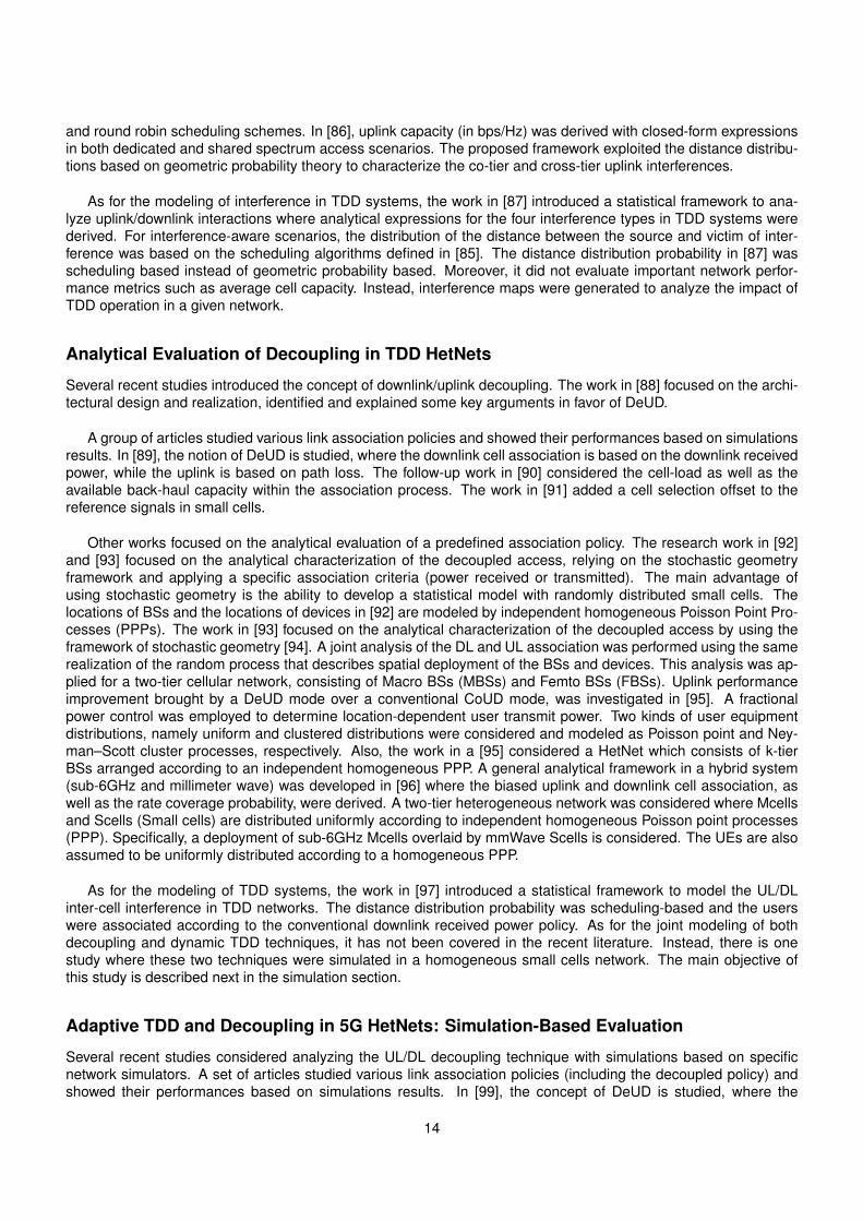
and round robin scheduling schemes. In [86], uplink capacity (in bps/Hz) was derived with closed-form expressionsin both dedicated and shared spectrum access scenarios. The proposed framework exploited the distance distribu-tions based on geometric probability theory to characterize the co-tier and cross-tier uplink interferences.
As for the modeling of interference in TDD systems, the work in [87] introduced a statistical framework to ana-lyze uplink/downlink interactions where analytical expressions for the four interference types in TDD systems werederived. For interference-aware scenarios, the distribution of the distance between the source and victim of inter-ference was based on the scheduling algorithms defined in [85]. The distance distribution probability in [87] wasscheduling based instead of geometric probability based. Moreover, it did not evaluate important network perfor-mance metrics such as average cell capacity. Instead, interference maps were generated to analyze the impact ofTDD operation in a given network.
Analytical Evaluation of Decoupling in TDD HetNets
Several recent studies introduced the concept of downlink/uplink decoupling. The work in [88] focused on the archi-tectural design and realization, identified and explained some key arguments in favor of DeUD.
A group of articles studied various link association policies and showed their performances based on simulationsresults. In [89], the notion of DeUD is studied, where the downlink cell association is based on the downlink receivedpower, while the uplink is based on path loss. The follow-up work in [90] considered the cell-load as well as theavailable back-haul capacity within the association process. The work in [91] added a cell selection offset to thereference signals in small cells.
Other works focused on the analytical evaluation of a predefined association policy. The research work in [92]and [93] focused on the analytical characterization of the decoupled access, relying on the stochastic geometryframework and applying a specific association criteria (power received or transmitted). The main advantage ofusing stochastic geometry is the ability to develop a statistical model with randomly distributed small cells. Thelocations of BSs and the locations of devices in [92] are modeled by independent homogeneous Poisson Point Pro-cesses (PPPs). The work in [93] focused on the analytical characterization of the decoupled access by using theframework of stochastic geometry [94]. A joint analysis of the DL and UL association was performed using the samerealization of the random process that describes spatial deployment of the BSs and devices. This analysis was ap-plied for a two-tier cellular network, consisting of Macro BSs (MBSs) and Femto BSs (FBSs). Uplink performanceimprovement brought by a DeUD mode over a conventional CoUD mode, was investigated in [95]. A fractionalpower control was employed to determine location-dependent user transmit power. Two kinds of user equipmentdistributions, namely uniform and clustered distributions were considered and modeled as Poisson point and Ney-man–Scott cluster processes, respectively. Also, the work in a [95] considered a HetNet which consists of k-tierBSs arranged according to an independent homogeneous PPP. A general analytical framework in a hybrid system(sub-6GHz and millimeter wave) was developed in [96] where the biased uplink and downlink cell association, aswell as the rate coverage probability, were derived. A two-tier heterogeneous network was considered where Mcellsand Scells (Small cells) are distributed uniformly according to independent homogeneous Poisson point processes(PPP). Specifically, a deployment of sub-6GHz Mcells overlaid by mmWave Scells is considered. The UEs are alsoassumed to be uniformly distributed according to a homogeneous PPP.
As for the modeling of TDD systems, the work in [97] introduced a statistical framework to model the UL/DLinter-cell interference in TDD networks. The distance distribution probability was scheduling-based and the userswere associated according to the conventional downlink received power policy. As for the joint modeling of bothdecoupling and dynamic TDD techniques, it has not been covered in the recent literature. Instead, there is onestudy where these two techniques were simulated in a homogeneous small cells network. The main objective ofthis study is described next in the simulation section.
Adaptive TDD and Decoupling in 5G HetNets: Simulation-Based Evaluation
Several recent studies considered analyzing the UL/DL decoupling technique with simulations based on specificnetwork simulators. A set of articles studied various link association policies (including the decoupled policy) andshowed their performances based on simulations results. In [99], the concept of DeUD is studied, where the
14
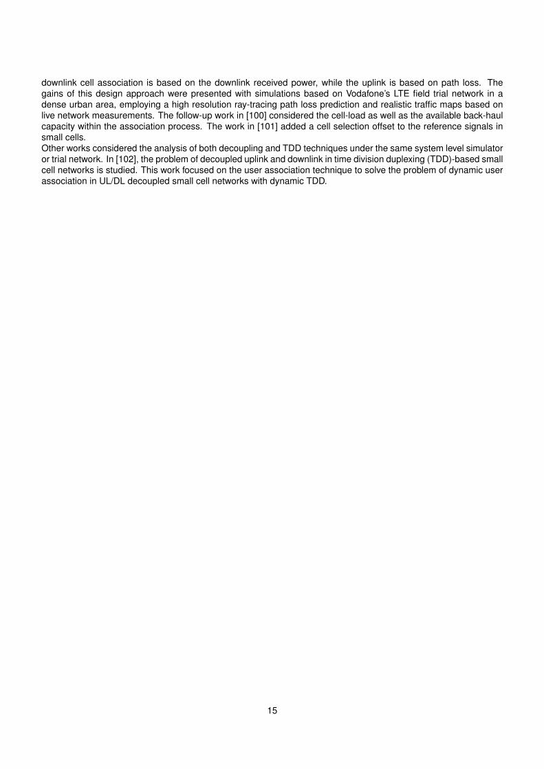
downlink cell association is based on the downlink received power, while the uplink is based on path loss. Thegains of this design approach were presented with simulations based on Vodafone’s LTE field trial network in adense urban area, employing a high resolution ray-tracing path loss prediction and realistic traffic maps based onlive network measurements. The follow-up work in [100] considered the cell-load as well as the available back-haulcapacity within the association process. The work in [101] added a cell selection offset to the reference signals insmall cells.Other works considered the analysis of both decoupling and TDD techniques under the same system level simulatoror trial network. In [102], the problem of decoupled uplink and downlink in time division duplexing (TDD)-based smallcell networks is studied. This work focused on the user association technique to solve the problem of dynamic userassociation in UL/DL decoupled small cell networks with dynamic TDD.
15
2.2 Thesis Contributions
The main contributions of this work can be summarized as follows:
1) TDD Statistical Model: We consider analyzing, in this work, both uplink/downlink interactions, whereas otherworks introduced either a downlink ICI model as in [76] and [77] or an uplink ICI model as in [85] and [86].Few studies considered modeling a TDD system, however they either did not consider a HetNet system ordid not evaluate any network performance indicator as in [87]. In this work, operating a TDD-based HetNetnetwork necessitates four interference scenarios depending mainly on the geographical distance between thereference cell and the neighboring cell. In a multiple small cells scenario, the neighboring cell can be eitherthe small cell or the macro cell. Thus, analyzing four interference scenarios is still applicable because of theTDD subframes distribution that is considered perfectly synchronized between the small cells (See Table 2.1for illustration).
TDD
UL InteractionsModel
DL InteractionsModel TDD Model HetNets
Total Though-puts (UL andDL)
[75] K. W. Sung, H. Haas, and S. McLaughlin, “A semi-analyticalPDF of downlink SINR for femtocell networks,” EURASIP J. Wire-less Commun. and Networking, Jan. 2010.
XXX
[76] S. Plass, X. G. Doukopoulos, and R. Legouable, “Investiga-tions on link-level inter-cell interference in OFDMA systems,” inProc. 2006 IEEE Symposium on Communications and VehicularTechnology, pp. 49-52.
XXX
[77] X. Yang and A. O. Fapojuwo, “Analysis of heterogeneous cel-lular network with hexagonal tessellated macrocells and randomlypositioned small cells,” IEEE WCNC, 2016.
XXX XXX
[78] M. Taranetz and M. Rupp, “A circular interference model forwireless cellular networks,” International Wireless Communicationsand Mobile Computing Conference, 2014.
XXX
[81] S. Elayoubi, B. Haddada, and B. Fourestie, “Performanceevaluation of fre- quency planning schemes in OFDMA based net-works,” IEEE Trans.Wireless Commun., vol. 7, no. 5, pp. 1623-1633, May 2008.
XXX
[82] R. Kwan and C. Leung, “On collision probabilities infrequency-domain scheduling for LTE cellular networks,” IEEECommun. Lett., vol. 15, no. 9, pp. 965- 967, Sep. 2011.
XXX
TDDModel
[83] I. Viering, A. Klein, M. Ivrlac, M. Castaneda, and J. A. Nossek,“On uplink intercell interference in a cellular system,” in Proc. 2006IEEE International Conference on Communications, pp. 2095-2100.
XXX
[84] M. Ding, D. Lopez-Perez, G. Mao, and Z. Lin, “DNA-GA: Anew approach of network performance analysis,” Proc. IEEE ICC2016,arXiv:1512.05429 [cs.IT], to be published.
XXX
[85] H. Tabassum, Z. Dawy, E. Hossain, and M. S Alouini, “Aframework for uplink intercell interference modeling with channel-based scheduling,”IEEE Trans. Wireless Commun., vol. 12, no. 1,pp. 206-217, Jan. 2013.
XXX
[86] H. Tabassum, Z. Dawy, E. Hossain, and M. S Alouini, “In-terference statistics and capacity analysis for uplink transmissionin two-tier small cell networks: A geometric probability approach,”IEEE Trans. Wireless Commun., vol. 13, no. 7, pp. 3837-3852,Jul. 2014.
XXX XXX
[87] Ahmad El-Hajj, Naeem Akl, Bilal Hammoud, and Zaher Dawy,“On interference modeling for the analysis of uplink/downlink in-teractions in TDD-OFDMA networks,” 2015 International WirelessCommunications and Mobile Computing Conference (IWCMC), pp.497-502, 2015.
XXX XXX XXX
[103] B. Lahad, M. Ibrahim, S. Lahoud, K. Khawam and S. Martin,“A Statistical Model for Uplink/Downlink Intercell Interference andCell Capacity in TDD HetNets”, ICC 2018: 1-6.
XXX XXX XXX XXX XXX
Table 2.1: Modeling a TDD-based HetNet [Related Work and Contribution].
16
2) Analytical Model Covering Various User Association Policies: Focusing on the decoupled access strategy,other similar works either developed an analytical model studying one specific association criteria ( [92]-[96]) or investigated multiple association strategies based on simulation results ( [89]- [91]). In this work, ananalytical model covering four association policies is developed with the aim of studying the improvementthat the decoupling access can bring to TDD HetNets among all other association policies (See Table 2.2 forillustration).
DecouplingDecoupling withVarious Associ-ation Policies
Analytical Eval-uation of De-coupling
[89] H. Elshaer, F. Boccardi, M. Dohler, and R. Irmer, “Downlinkand uplink decoupling: a disruptive architectural design for 5G net-works,” in GLOBECOM14. IEEE, 2014, pp. 1798-1803.
XXX
[90] “Load & backhaul aware decoupled downlink/uplink access in5G systems,” arXiv preprint arXiv:1410.6680, 2014. XXX
[91] Qualcomm, “Range expansion for efficient support of hetero-geneous networks,” 3GPP TSG-RAN WG1 R1-083813, 2008 XXX
[92] K. Smiljkovikj, H. Elshaer, P. Popovski, F. Boccardi, M. Dohler,L. Gavrilovska, and R. Irmer, “Capacity analysis of decoupleddownlink and uplink access in 5G heterogeneous systems,” arXivpreprint arXiv:1410.7270, 2014.
XXX
UL/DL DecoupledAccess
[93] K. Smiljkovikj, P. Popovski, and L. Gavrilovska, “Analysis ofthe decoupled access for downlink and uplink in wireless hetero-geneous networks,” Wireless Communications Letters, IEEE, vol.4, no. 2, pp. 173-176, 2015.
XXX
[95] W. Nie, L. Zhang, and G. Fang, “Uplink Performance Improve-ment by Decoupling Uplink/Downlink Access in HetNets,” IEEETransactions on Vehicular Technology, IEEE, vol. 66, no. 8, pp.6862-6876, 2017.
XXX
[96] H. E. Shaer, M. N. Kulkarni, F. Boccardi, J. G. Andrews, andM. Dohler, “Downlink and Uplink Cell Association in Sub-6GHz andMillimeter Wave 5G Heterogeneous Networks,” Globecom Work-shops (GC Wkshps), 2016 IEEE.
XXX
[117] B. Lahad, M. Ibrahim, S. Lahoud, K. Khawam and S. Martin,“Analytical Evaluation of Decoupled Uplink and Downlink Accessin TDD 5G HetNets”, PIMRC 2018: 1-7.
XXX XXX
Table 2.2: Analytical model covering various user association policies [Related Work and Contribution].
3) Joint Modeling of TDD and Decoupled UL/DL access in Multiple Small Cells HetNets: Studying the next-generation wireless 5G HetNets with respect to TDD and UL/DL decoupled access. Other works investigatedeither a TDD system as in [87] and [103] or the decoupled access technique as in [89]- [96]. In fact, consideringa TDD model jointly with a decoupled association policy appears to be a viable solution to address UL and DLthroughput degradation challenges (See Table 2.3 for illustration). The work in [117] studied both decouplingand TDD techniques, however it was limited to one small cell case study.In our model, we consider a network consisting of one macro cell along with a reference small cell located ata certain distance from the macro cell. Multiple instances of interfering small cells are deployed at specificdistances from the reference small cell in order to be aligned as much as possible with real case scenarios. Weconsider this specific network model, as simple as it shows in regards to BS distribution, to focus on the mainthesis objective which is the modeling of TDD and decoupling in a scenario that is close to real cases, and atthe same time to avoid adding further complexity to the model itself. Instead, including any other BS distribution(stochastic for example), will bring significant additional complexity to our HetNet analysis, especially that ouraim is to combine both decoupling and dynamic TDD techniques under one statistical model. Our model isbased on geometric approach contrary to most of the recent articles, where the model is based on stochasticprobability and the user association is based on UL/DL received power. However, we will rely on the recentliterature on decoupling ( [104], [105]) to retrieve the small cell bias/offset (power based) and apply it in oursystem level simulations that analyze different association policies among them, a power based policy. Thelatter will be discussed in details in Chapter5.
17
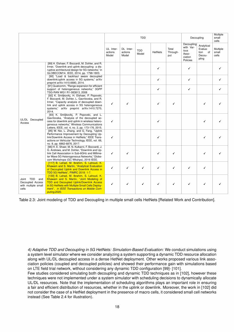
TDD DecouplingMultiplesmallcells
UL Inter-actionsModel
DL Inter-actionsModel
TDDModel HetNets
TotalThrough-put
Decouplingwith Var-iousAsso-ciationPolicies
AnalyticalEvalua-tion ofDecou-pling
Multiplesmallcells
[89] H. Elshaer, F. Boccardi, M. Dohler, and R.Irmer, “Downlink and uplink decoupling: a dis-ruptive architectural design for 5G networks,” inGLOBECOM14. IEEE, 2014, pp. 1798-1803.
XXX XXX XXX
[90] “Load & backhaul aware decoupleddownlink/uplink access in 5G systems,” arXivpreprint arXiv:1410.6680, 2014.
XXX XXX XXX
[91] Qualcomm, “Range expansion for efficientsupport of heterogeneous networks,” 3GPPTSG-RAN WG1 R1-083813, 2008
XXX XXX XXX
[92] K. Smiljkovikj, H. Elshaer, P. Popovski,F. Boccardi, M. Dohler, L. Gavrilovska, and R.Irmer, “Capacity analysis of decoupled down-link and uplink access in 5G heterogeneoussystems,” arXiv preprint arXiv:1410.7270,2014.
XXX XXX XXX XXX XXX XXX
UL/DL DecoupledAccess
[93] K. Smiljkovikj, P. Popovski, and L.Gavrilovska, “Analysis of the decoupled ac-cess for downlink and uplink in wireless hetero-geneous networks,” Wireless CommunicationsLetters, IEEE, vol. 4, no. 2, pp. 173-176, 2015.
XXX XXX XXX XXX
[95] W. Nie, L. Zhang, and G. Fang, “UplinkPerformance Improvement by Decoupling Up-link/Downlink Access in HetNets,” IEEE Trans-actions on Vehicular Technology, IEEE, vol. 66,no. 8, pp. 6862-6876, 2017.
XXX XXX XXX XXX
[96] H. E. Shaer, M. N. Kulkarni, F. Boccardi, J.G. Andrews, and M. Dohler, “Downlink and Up-link Cell Association in Sub-6GHz and Millime-ter Wave 5G Heterogeneous Networks,” Globe-com Workshops (GC Wkshps), 2016 IEEE.
XXX XXX XXX XXX XXX XXX
[117] B. Lahad, M. Ibrahim, S. Lahoud, K.Khawam and S. Martin, “Analytical Evaluationof Decoupled Uplink and Downlink Access inTDD 5G HetNets”, PIMRC 2018: 1-7.
XXX XXX XXX XXX XXX XXX XXX
Joint TDD andDecoupled Accesswith multiple smallcells
[130] B. Lahad, M. Ibrahim, S. Lahoud, K.Khawam and S. Martin, “Joint Modeling ofTDD and Decoupled Uplink/Downlink Accessin 5G HetNets with Multiple Small Cells Deploy-ment”, in IEEE Transactions on Mobile Com-puting,2020.
XXX XXX XXX XXX XXX XXX XXX XXX
Table 2.3: Joint modeling of TDD and Decoupling in multiple small cells HetNets [Related Work and Contribution].
4) Adaptive TDD and Decoupling in 5G HetNets: Simulation-Based Evaluation: We conduct simulations usinga system level simulator where we consider analyzing a system supporting a dynamic TDD resource allocationalong with UL/DL decoupled access in a dense HetNet deployment. Other works proposed various link asso-ciation policies (coupled and decoupled policies) and showed their performance gain with simulations basedon LTE field trial network, without considering any dynamic TDD configuration [99]- [101].Few studies considered simulating both decoupling and dynamic TDD techniques as in [102], however thesetechniques were not implemented under a system simulator with scheduling decisions to dynamically allocateUL/DL resources. Note that the implementation of scheduling algorithms plays an important role in ensuringa fair and efficient distribution of resources, whether in the uplink or downlink. Moreover, the work in [102] didnot consider the case of a HetNet deployment in the presence of macro cells, it considered small cell networksinstead (See Table 2.4 for illustration).
18
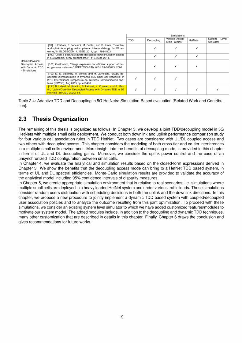
Simulations
TDD Decoupling Various Associ-ation Policies HetNets System Level
Simulator[99] H. Elshaer, F. Boccardi, M. Dohler, and R. Irmer, “Downlink
and uplink decoupling: a disruptive architectural design for 5G net-works,” in GLOBECOM14. IEEE, 2014, pp. 1798-1803.
XXX XXX XXX
[100] “Load & backhaul aware decoupled downlink/uplink accessin 5G systems,” arXiv preprint arXiv:1410.6680, 2014. XXX XXX XXX
Uplink/DownlinkDecoupled Accesswith Dynamic TDD- Simulations
[101] Qualcomm, “Range expansion for efficient support of het-erogeneous networks,” 3GPP TSG-RAN WG1 R1-083813, 2008 XXX XXX XXX
[102] M. S. ElBamby, M. Bennis, and M. Latva-aho, “UL/DL de-coupled userassociation in dynamic TDD small cell networks,” in2015 International Symposium on Wireless Communication Sys-tems (ISWCS), Aug 2015,pp. 456460.
XXX XXX XXX
[131] B. Lahad, M. Ibrahim, S. Lahoud, K. Khawam and S. Mar-tin, “Uplink/Downlink Decoupled Access with Dynamic TDD in 5GHetNets”, IWCMC 2020: 1-6.
XXX XXX XXX XXX XXX
Table 2.4: Adaptive TDD and Decoupling in 5G HetNets: Simulation-Based evaluation [Related Work and Contribu-tion].
2.3 Thesis Organization
The remaining of this thesis is organized as follows: In Chapter 3, we develop a joint TDD/decoupling model in 5GHetNets with multiple small cells deployment. We conduct both downlink and uplink performance comparison studyfor four various cell association rules in TDD HetNet. Two cases are considered with UL/DL coupled access andtwo others with decoupled access. This chapter considers the modeling of both cross-tier and co-tier interferencesin a multiple small cells environment. More insight into the benefits of decoupling mode, is provided in this chapterin terms of UL and DL decoupling gains. Moreover, we consider the uplink power control and the case of anunsynchronized TDD configuration between small cells.In Chapter 4, we evaluate the analytical and simulation results based on the closed-form expressions derived inChapter 3. We show the benefits that the decoupling access mode can bring to a HetNet TDD based system, interms of UL and DL spectral efficiencies. Monte-Carlo simulation results are provided to validate the accuracy ofthe analytical model including 95% confidence intervals of disparity measures.In Chapter 5, we create appropriate simulation environment that is relative to real scenarios, i.e. simulations wheremultiple small cells are deployed in a heavy loaded HetNet system and under various traffic loads. These simulationsconsider random users distribution with scheduling decisions in both the uplink and the downlink directions. In thischapter, we propose a new procedure to jointly implement a dynamic TDD based system with coupled/decoupleduser association policies and to analyze the outcome resulting from this joint optimization. To proceed with thesesimulations, we consider an existing system level simulator to which we have added customized features/modules tomotivate our system model. The added modules include, in addition to the decoupling and dynamic TDD techniques,many other customization that are described in details in this chapter. Finally, Chapter 6 draws the conclusion andgives recommendations for future works.
19

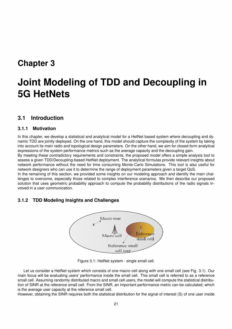
Chapter 3
Joint Modeling of TDD and Decoupling in5G HetNets
3.1 Introduction
3.1.1 Motivation
In this chapter, we develop a statistical and analytical model for a HetNet based system where decoupling and dy-namic TDD are jointly deployed. On the one hand, this model should capture the complexity of the system by takinginto account its main radio and topological design parameters. On the other hand, we aim for closed-form analyticalexpressions of the system performance metrics such as the average capacity and the decoupling gain.By meeting these contradictory requirements and constraints, the proposed model offers a simple analysis tool toassess a given TDD/Decoupling-based HetNet deployment. The analytical formulas provide relevant insights aboutnetwork performance without the need for time consuming Monte-Carlo Simulations. This tool is also useful fornetwork designers who can use it to determine the range of deployment parameters given a target QoS.In the remaining of this section, we provided some insights on our modeling approach and identify the main chal-lenges to overcome, especially those related to complex interference scenarios. We then describe our proposedsolution that uses geometric probability approach to compute the probability distributions of the radio signals in-volved in a user communication.
3.1.2 TDD Modeling Insights and Challenges
Figure 3.1: HetNet system - single small cell.
Let us consider a HetNet system which consists of one macro cell along with one small cell (see Fig. 3.1). Ourmain focus will be evaluating users’ performance inside the small cell. This small cell is referred to as a referencesmall cell. Assuming randomly distributed macro and small cell users, the model will compute the statistical distribu-tion of SINR at the reference small cell. From the SINR, an important performance metric can be calculated, whichis the average user capacity at the reference small cell.However, obtaining the SINR requires both the statistical distribution for the signal of interest (S) of one user inside
21
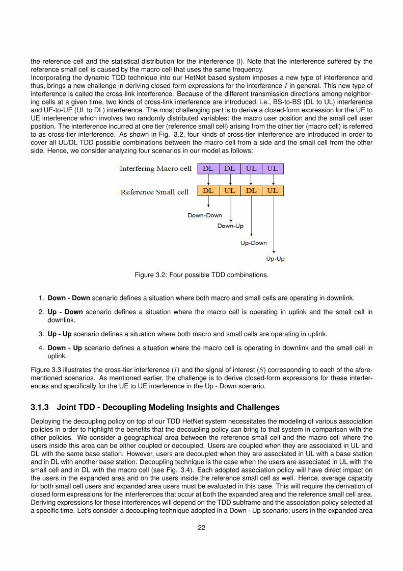
the reference cell and the statistical distribution for the interference (I). Note that the interference suffered by thereference small cell is caused by the macro cell that uses the same frequency.Incorporating the dynamic TDD technique into our HetNet based system imposes a new type of interference andthus, brings a new challenge in deriving closed-form expressions for the interference I in general. This new type ofinterference is called the cross-link interference. Because of the different transmission directions among neighbor-ing cells at a given time, two kinds of cross-link interference are introduced, i.e., BS-to-BS (DL to UL) interferenceand UE-to-UE (UL to DL) interference. The most challenging part is to derive a closed-form expression for the UE toUE interference which involves two randomly distributed variables: the macro user position and the small cell userposition. The interference incurred at one tier (reference small cell) arising from the other tier (macro cell) is referredto as cross-tier interference. As shown in Fig. 3.2, four kinds of cross-tier interference are introduced in order tocover all UL/DL TDD possible combinations between the macro cell from a side and the small cell from the otherside. Hence, we consider analyzing four scenarios in our model as follows:
Figure 3.2: Four possible TDD combinations.
1. Down - Down scenario defines a situation where both macro and small cells are operating in downlink.
2. Up - Down scenario defines a situation where the macro cell is operating in uplink and the small cell indownlink.
3. Up - Up scenario defines a situation where both macro and small cells are operating in uplink.
4. Down - Up scenario defines a situation where the macro cell is operating in downlink and the small cell inuplink.
Figure 3.3 illustrates the cross-tier interference (I) and the signal of interest (S) corresponding to each of the afore-mentioned scenarios. As mentioned earlier, the challenge is to derive closed-form expressions for these interfer-ences and specifically for the UE to UE interference in the Up - Down scenario.
3.1.3 Joint TDD - Decoupling Modeling Insights and Challenges
Deploying the decoupling policy on top of our TDD HetNet system necessitates the modeling of various associationpolicies in order to highlight the benefits that the decoupling policy can bring to that system in comparison with theother policies. We consider a geographical area between the reference small cell and the macro cell where theusers inside this area can be either coupled or decoupled. Users are coupled when they are associated in UL andDL with the same base station. However, users are decoupled when they are associated in UL with a base stationand in DL with another base station. Decoupling technique is the case when the users are associated in UL with thesmall cell and in DL with the macro cell (see Fig. 3.4). Each adopted association policy will have direct impact onthe users in the expanded area and on the users inside the reference small cell as well. Hence, average capacityfor both small cell users and expanded area users must be evaluated in this case. This will require the derivation ofclosed form expressions for the interferences that occur at both the expanded area and the reference small cell area.Deriving expressions for these interferences will depend on the TDD subframe and the association policy selected ata specific time. Let’s consider a decoupling technique adopted in a Down - Up scenario; users in the expanded area
22
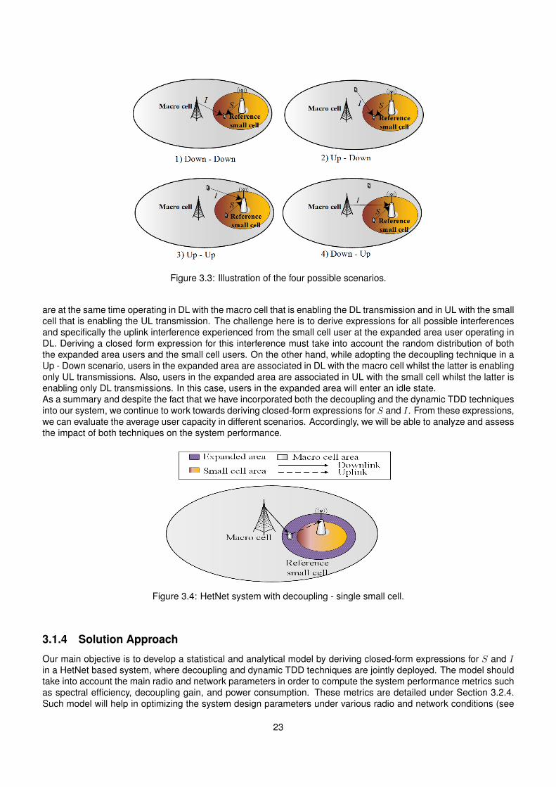
Figure 3.3: Illustration of the four possible scenarios.
are at the same time operating in DL with the macro cell that is enabling the DL transmission and in UL with the smallcell that is enabling the UL transmission. The challenge here is to derive expressions for all possible interferencesand specifically the uplink interference experienced from the small cell user at the expanded area user operating inDL. Deriving a closed form expression for this interference must take into account the random distribution of boththe expanded area users and the small cell users. On the other hand, while adopting the decoupling technique in aUp - Down scenario, users in the expanded area are associated in DL with the macro cell whilst the latter is enablingonly UL transmissions. Also, users in the expanded area are associated in UL with the small cell whilst the latter isenabling only DL transmissions. In this case, users in the expanded area will enter an idle state.As a summary and despite the fact that we have incorporated both the decoupling and the dynamic TDD techniquesinto our system, we continue to work towards deriving closed-form expressions for S and I. From these expressions,we can evaluate the average user capacity in different scenarios. Accordingly, we will be able to analyze and assessthe impact of both techniques on the system performance.
Figure 3.4: HetNet system with decoupling - single small cell.
3.1.4 Solution Approach
Our main objective is to develop a statistical and analytical model by deriving closed-form expressions for S and Iin a HetNet based system, where decoupling and dynamic TDD techniques are jointly deployed. The model shouldtake into account the main radio and network parameters in order to compute the system performance metrics suchas spectral efficiency, decoupling gain, and power consumption. These metrics are detailed under Section 3.2.4.Such model will help in optimizing the system design parameters under various radio and network conditions (see
23
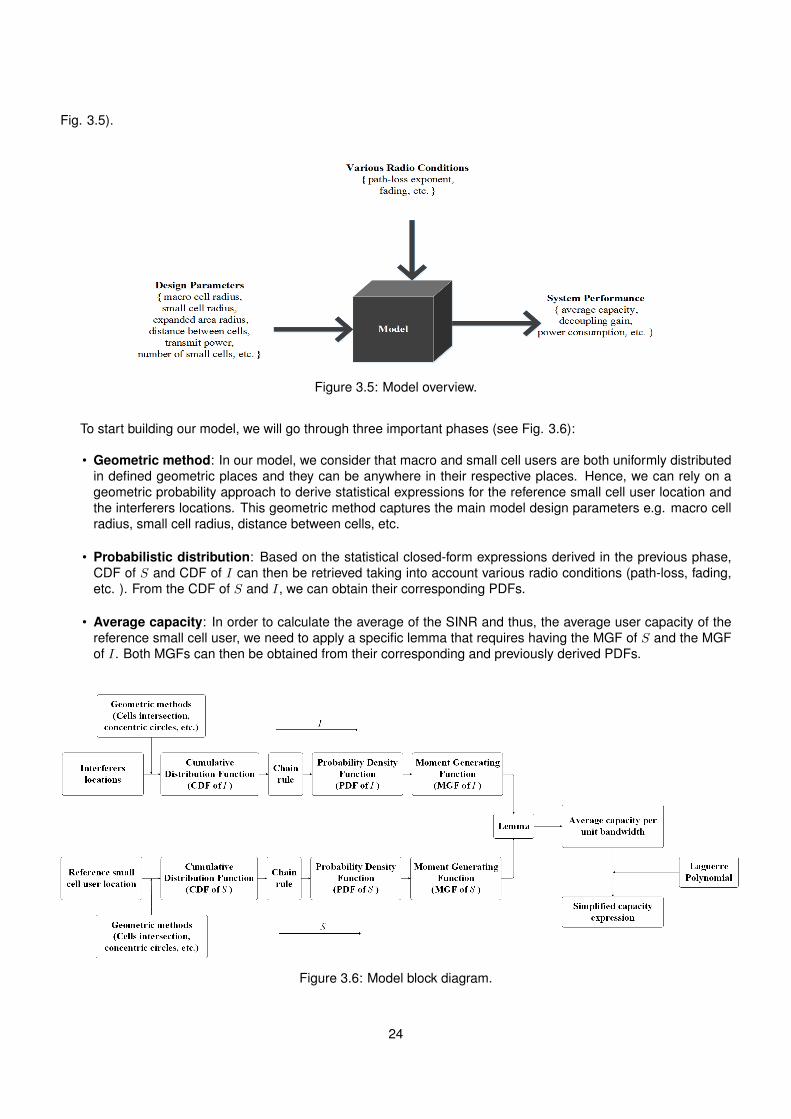
Fig. 3.5).
Figure 3.5: Model overview.
To start building our model, we will go through three important phases (see Fig. 3.6):
• Geometric method: In our model, we consider that macro and small cell users are both uniformly distributedin defined geometric places and they can be anywhere in their respective places. Hence, we can rely on ageometric probability approach to derive statistical expressions for the reference small cell user location andthe interferers locations. This geometric method captures the main model design parameters e.g. macro cellradius, small cell radius, distance between cells, etc.
• Probabilistic distribution: Based on the statistical closed-form expressions derived in the previous phase,CDF of S and CDF of I can then be retrieved taking into account various radio conditions (path-loss, fading,etc. ). From the CDF of S and I, we can obtain their corresponding PDFs.
• Average capacity: In order to calculate the average of the SINR and thus, the average user capacity of thereference small cell user, we need to apply a specific lemma that requires having the MGF of S and the MGFof I. Both MGFs can then be obtained from their corresponding and previously derived PDFs.
Figure 3.6: Model block diagram.
24
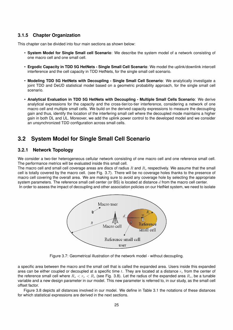
3.1.5 Chapter Organization
This chapter can be divided into four main sections as shown below:
• System Model for Single Small cell Scenario: We describe the system model of a network consisting ofone macro cell and one small cell.
• Ergodic Capacity in TDD 5G HetNets - Single Small Cell Scenario: We model the uplink/downlink intercellinterference and the cell capacity in TDD HetNets, for the single small cell scenario.
• Modeling TDD 5G HetNets with Decoupling - Single Small Cell Scenario: We analytically investigate ajoint TDD and DeUD statistical model based on a geometric probability approach, for the single small cellscenario.
• Analytical Evaluation in TDD 5G HetNets with Decoupling - Multiple Small Cells Scenario: We deriveanalytical expressions for the capacity and the cross-tier/co-tier interference, considering a network of onemacro cell and multiple small cells. We build on the derived capacity expressions to measure the decouplinggain and thus, identify the location of the interfering small cell where the decoupled mode maintains a highergain in both DL and UL. Moreover, we add the uplink power control to the developed model and we consideran unsynchronized TDD configuration across small cells.
3.2 System Model for Single Small Cell Scenario
3.2.1 Network Topology
We consider a two-tier heterogeneous cellular network consisting of one macro cell and one reference small cell.The performance metrics will be evaluated inside this small cell.The macro cell and small cell coverage areas are discs of radius R and Rs respectively. We assume that the smallcell is totally covered by the macro cell. (see Fig. 3.7). There will be no coverage holes thanks to the presence ofmacro cell covering the overall area. We are making sure to avoid any coverage hole by selecting the appropriatesystem parameters. The reference small cell center (or BS) is located at distance d from the macro cell center.In order to assess the impact of decoupling and other association policies on our HetNet system, we need to isolate
Figure 3.7: Geometrical illustration of the network model - without decoupling.
a specific area between the macro and the small cell that is called the expanded area. Users inside this expandedarea can be either coupled or decoupled at a specific time t. They are located at a distance re from the center ofthe reference small cell where Rs < re < Re (see Fig. 3.8). Let the radius of the expanded area Re, be a tunablevariable and a new design parameter in our model. This new parameter is referred to, in our study, as the small celloffset factor.
Figure 3.8 depicts all distances involved in our model. We define in Table 3.1 the notations of these distancesfor which statistical expressions are derived in the next sections.
25
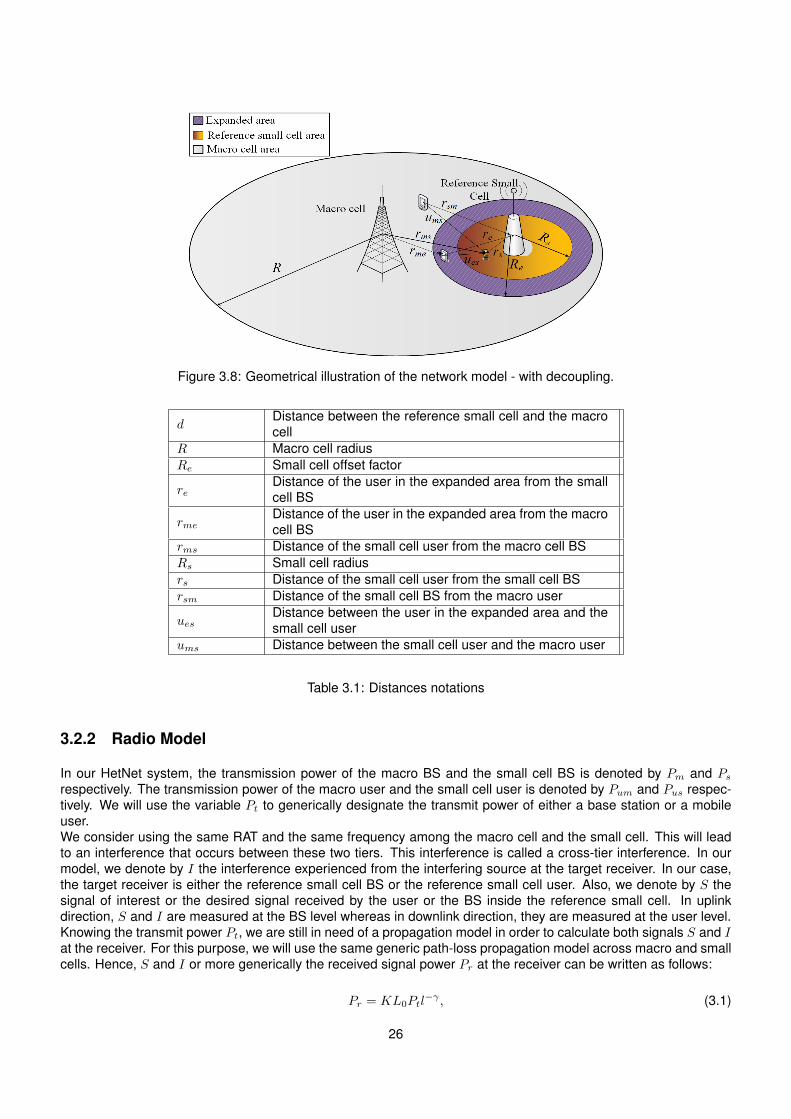
Figure 3.8: Geometrical illustration of the network model - with decoupling.
dDistance between the reference small cell and the macrocell
R Macro cell radiusRe Small cell offset factor
reDistance of the user in the expanded area from the smallcell BS
rmeDistance of the user in the expanded area from the macrocell BS
rms Distance of the small cell user from the macro cell BSRs Small cell radiusrs Distance of the small cell user from the small cell BSrsm Distance of the small cell BS from the macro user
uesDistance between the user in the expanded area and thesmall cell user
ums Distance between the small cell user and the macro user
Table 3.1: Distances notations
3.2.2 Radio Model
In our HetNet system, the transmission power of the macro BS and the small cell BS is denoted by Pm and Psrespectively. The transmission power of the macro user and the small cell user is denoted by Pum and Pus respec-tively. We will use the variable Pt to generically designate the transmit power of either a base station or a mobileuser.We consider using the same RAT and the same frequency among the macro cell and the small cell. This will leadto an interference that occurs between these two tiers. This interference is called a cross-tier interference. In ourmodel, we denote by I the interference experienced from the interfering source at the target receiver. In our case,the target receiver is either the reference small cell BS or the reference small cell user. Also, we denote by S thesignal of interest or the desired signal received by the user or the BS inside the reference small cell. In uplinkdirection, S and I are measured at the BS level whereas in downlink direction, they are measured at the user level.Knowing the transmit power Pt, we are still in need of a propagation model in order to calculate both signals S and Iat the receiver. For this purpose, we will use the same generic path-loss propagation model across macro and smallcells. Hence, S and I or more generically the received signal power Pr at the receiver can be written as follows:
Pr = KL0Ptl−γ , (3.1)
26
where K is the composite fading, L0 the path-loss constant, γ the path-loss exponent and l is the length of the radiolink between the transmitter and the receiver in meters. L0 depends on the carrier frequency and the propagationenvironment.Considering a suburban environment, the path-loss expression in dB can be written as follows [106] [107]:
PL(dB) = 122.08 + 20log10fc + 10γlog10l, (3.2)
where fc is the carrier frequency in GHz and l is the length of the radio link between the transmitter and the receiverin kilometers. L0 in (3.1) can be then retrieved by mapping (3.1) to (3.2) as follows:
PL(dB) = 10log10L0 − 10γlog10l = −122.08− 20log10fc − 10γlog10l
1000, (3.3)
where l is the length of the radio link between the transmitter and the receiver in meters.Since the users are randomly distributed inside macro and small cells, we can conclude that l is a random variable.Accordingly and based on (3.1), S and I will be two random variables as well.
Moreover, considering the dynamic TDD technique in our HetNet system imposes the analysis of the four sce-narios described previously in Section 3.1.1, and which are Down - Down, Up - Down, Down - Up and Up - Upscenarios. In our model, closed-form expressions for S and I will be derived in each of these scenarios.
Assumption 1. In this model, the composite fading denoted by K is considered as a constant. It combines boththe shadowing and the fast fading.Nonetheless, we have simulated exactly the same scenarios under random variable fading. A log-normal shadowingand an exponential distribution with parameter λ = 1 as an approximation of the Rayleigh fading, were considered.As a result, we obtained nearly the same throughput values in UL and DL and the same behavior as in the case ofa constant composite fading; the impact of the decoupling in comparison with other association policies remainedthe same. Consequently, a constant fading was adopted in this model. In the next chapter, we will assess and showthe impact of the variable fading under section 4.2.2.
Assumption 2. In this model, we consider the interference (I) and the signal of interest (S) as two statisticallyindependent random variables. To justify our assumption, we have statistically derived the correlation coefficient tomeasure the dependency between the two variables S and I. Referring to the path-loss formula in (3.1) and to theAssumption 1, we can conclude that S is a function of the reference small cell user position. In some rare cases, Imight be indirectly a function of the same reference small cell user position. Accordingly, some cases show exactlya zero correlation, others show nearly zero values.In the next chapter, we will show under section 4.3.1 the correlation between S and I in order to validate ourassumption.
3.2.3 Traffic Model
We consider uniformly distributed users in both macro and small cells. Hence, both the interference experiencedfrom one single user inside each interfering cell and the signal of interest of one single user inside the referencesmall cell, must be statistically derived. In this case, the total system bandwidth will be allocated to that single userin each cell, whether a macro or a small cell. This full load assumption characterizes our system traffic model.
3.2.4 Performance Metrics
In this model, we study several network performance metrics based on the expressions derived for the interferenceand the signal of interest. We present hereafter the definition and the motivation of each of these metrics:
Spectrum Efficiency or Ergodic Capacity per Unit Bandwidth
Spectrum efficiency (in bps/Hz) refers to the maximum information rate that can be transmitted over a given band-width in a specific communication system. With the surge of data traffic and limited spectrum resources, a highspectrum efficiency is a mandatory requirement of next generation networks. In our model, we consider analyzing
27
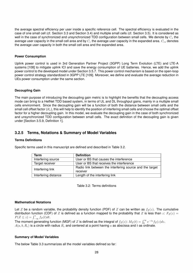
the average spectral efficiency per user inside a specific reference cell. The spectral efficiency is evaluated in thecase of one small cell (cf. Section 3.3 and Section 3.4) and multiple small cells (cf. Section 3.5). It is considered aswell in the case of synchronized and unsynchronized TDD configuration between small cells. We denote by Cs theaverage user capacity in the small cell area and by Ce the average user capacity in the expanded area. Ces denotesthe average user capacity in both the small cell area and the expanded area.
Power Consumption
Uplink power control is used in 3rd Generation Partner Project (3GPP) Long Term Evolution (LTE) and LTE-Asystems [108] to mitigate uplink ICI and save the energy consumption of UE batteries. Hence, we add the uplinkpower control to the developed model under Section 3.5.7. This power control mechanism is based on the open-looppower control strategy standardized in 3GPP LTE [109]. Moreover, we define and evaluate the average reduction inUEs power consumption under the same section.
Decoupling Gain
The main purpose of introducing the decoupling gain metric is to highlight the benefits that the decoupling accessmode can bring to a HetNet TDD based system, in terms of UL and DL throughput gains, mainly in a multiple smallcells environment. Since the decoupling gain will be a function of both the distance between small cells and thesmall cell offset factor (Re), this will help to identify the position of interfering small cells and choose the optimal offsetfactor for a higher decoupling gain. In this model, we evaluate the decoupling gain in the case of both synchronizedand unsynchronized TDD configuration between small cells. The exact definition of the decoupling gain is givenunder [Section 3.5.9, Definition 1].
3.2.5 Terms, Notations & Summary of Model Variables
Terms Definitions
Specific terms used in this manuscript are defined and described in Table 3.2.
Term DefinitionInterfering source User or BS that causes the interferenceTarget receiver User or BS that receives the interference
Interfering link Radio link between the interfering source and the targetreceiver
Interfering distance Length of the interfering link
Table 3.2: Terms definitions
Mathematical Notations
Let Z be a random variable, the probability density function (PDF) of Z can be written as fZ(z). The cumulativedistribution function (CDF) of Z is defined as a function mapped to the probability that Z is less than z: FZ(z) =P (Z ≤ z) =
∫ z−∞ fZ(t)dt.
The moment generating function (MGF) of Z is defined as the integral of fZ(z): MZ(t) =∫∞0e−tzfZ(z)dz.
A(a, b, Rc) is a circle with radius Rc and centered at a point having a as abscissa and b as ordinate.
Summary of Model Variables
The below Table 3.3 summarizes all the model variables defined so far:
28
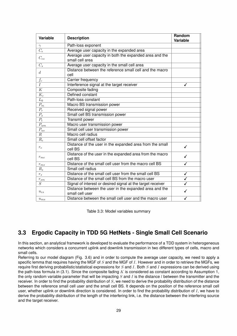
Variable Description RandomVariable
γ Path-loss exponentCe Average user capacity in the expanded area
CesAverage user capacity in both the expanded area and thesmall cell area
Cs Average user capacity in the small cell area
dDistance between the reference small cell and the macrocell
fc Carrier frequencyI Interference signal at the target receiver XXXK Composite fadingKc Defined constantL0 Path-loss constantPm Macro BS transmission powerPr Received signal powerPs Small cell BS transmission powerPt Transmit powerPum Macro user transmission powerPus Small cell user transmission powerR Macro cell radiusRe Small cell offset factor
reDistance of the user in the expanded area from the smallcell BS XXX
rmeDistance of the user in the expanded area from the macrocell BS XXX
rms Distance of the small cell user from the macro cell BS XXXRs Small cell radiusrs Distance of the small cell user from the small cell BS XXXrsm Distance of the small cell BS from the macro user XXXS Signal of interest or desired signal at the target receiver XXX
uesDistance between the user in the expanded area and thesmall cell user XXX
ums Distance between the small cell user and the macro user XXX
Table 3.3: Model variables summary
3.3 Ergodic Capacity in TDD 5G HetNets - Single Small Cell Scenario
In this section, an analytical framework is developed to evaluate the performance of a TDD system in heterogeneousnetworks which considers a concurrent uplink and downlink transmission in two different types of cells, macro andsmall cells.Referring to our model diagram (Fig. 3.6) and in order to compute the average user capacity, we need to apply aspecific lemma that requires having the MGF of S and the MGF of I. However and in order to retrieve the MGFs, werequire first deriving probabilistic/statistical expressions for S and I. Both S and I expressions can be derived usingthe path-loss formula in (3.1). Since the composite fading K is considered as constant according to Assumption 1,the only random variable parameter that will be impacting S and I is the distance l between the transmitter and thereceiver. In order to find the probability distribution of S, we need to derive the probability distribution of the distancebetween the reference small cell user and the small cell BS. It depends on the position of the reference small celluser, whether uplink or downlink direction is considered. In order to find the probability distribution of I, we have toderive the probability distribution of the length of the interfering link, i.e. the distance between the interfering sourceand the target receiver.
29
In this section, we will show how statistical expressions for both the reference user position and the interfering linklength can be derived using the proposed geometric approach.
3.3.1 Signal of Interest Modeling
A. Downlink Direction
The signal power received by a randomly selected user at the reference small cell on a downlink channel is definedusing equation (3.1) with Pt = Ps the transmit power and l = rs the reference user position. Consequently, S canbe written as follows:
S = KL0Psr−γs , (3.4)
Since we consider uniformly distributed users, the distribution of the distance rs of a small cell user will be followingthe distribution of a random point inside a disk of radius Rs:
frs(r) =2r
R2s
, 0 ≤ r ≤ Rs, (3.5)
According to Assumption 1, K is considered as constant. Consequently, the CDF of S can be formulated as:
FS(s) = P (S ≤ s) = P (KL0Psr−γs ≤ s) = P (r−γs ≤ s
KL0Ps) = P
(rs ≤ (
s
KL0Ps)−
1γ
)= 1− Frs
((s
Kc)−
1γ
), (3.6)
where Kc = KL0Ps and Frs(r) is the CDF of rs.
Applying the chain rule [111], the PDF of the received signal S can be formulated as:
fS(s) =1
sγfrs
((s
Kc)−
1γ
)(s
Kc)
−1γ . (3.7)
By replacing (3.5) in (3.7), the PDF of S can be written as:
fS(s) = βs−(2+γγ ), (3.8)
where β = 2K2γc
γR2s
.
Consequently, the MGF of S can be given as:
MS(t) = E[e(−tS)] =∫ ∞0
e−tsfS(s)ds. (3.9)
MS(t) =
∫ ∞a
βs−(2+γγ )e−tsds, (3.10)
where a = KcR−γs .
B. Uplink Direction
When the small cell is operating in uplink mode, the signal power received at the reference small cell on an uplinkchannel from a randomly selected user is defined using equation (3.1) with Pt = Pus and l = rs. Same formulas areapplied to the PDF and MGF of the signal of interest while changing the constant Kc to Kc = KL0Pus.
3.3.2 Interference Modeling
In order to characterize the statistics of each interference scenario that could occur in TDD-based HetNets, theproposed framework analyzes in details both the downlink and uplink interferences (see Fig. 3.9). This will requireconsidering the four interference scenarios described previously: Down - Down, Up - Down, Down - Up and Up -
30
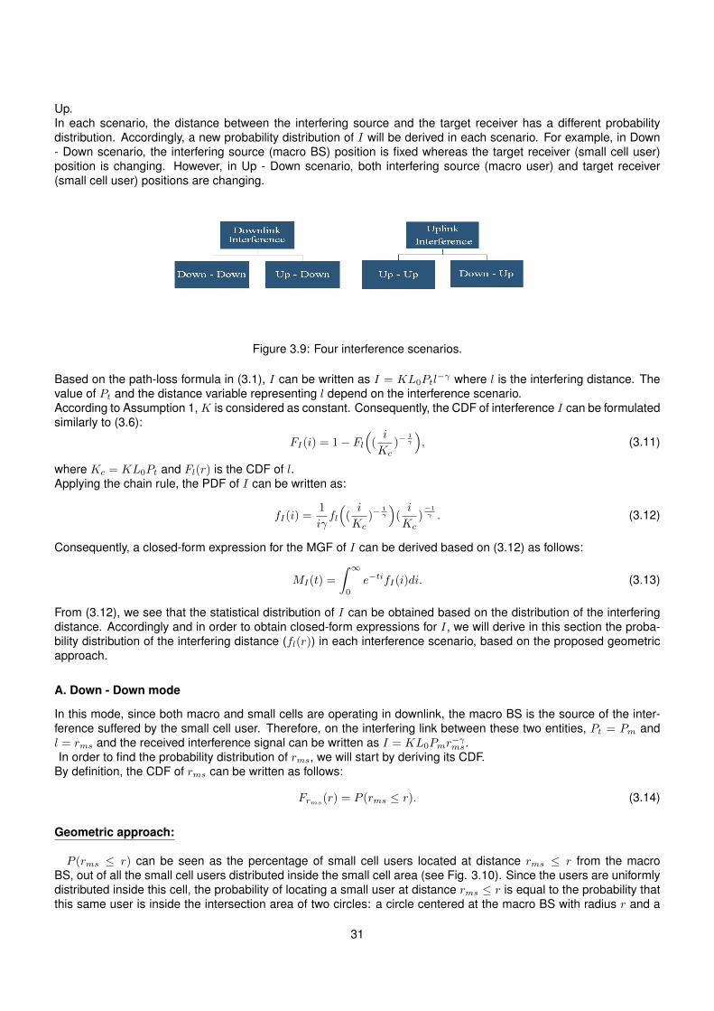
Up.In each scenario, the distance between the interfering source and the target receiver has a different probabilitydistribution. Accordingly, a new probability distribution of I will be derived in each scenario. For example, in Down- Down scenario, the interfering source (macro BS) position is fixed whereas the target receiver (small cell user)position is changing. However, in Up - Down scenario, both interfering source (macro user) and target receiver(small cell user) positions are changing.
Figure 3.9: Four interference scenarios.
Based on the path-loss formula in (3.1), I can be written as I = KL0Ptl−γ where l is the interfering distance. The
value of Pt and the distance variable representing l depend on the interference scenario.According to Assumption 1, K is considered as constant. Consequently, the CDF of interference I can be formulatedsimilarly to (3.6):
FI(i) = 1− Fl((i
Kc)−
1γ
), (3.11)
where Kc = KL0Pt and Fl(r) is the CDF of l.Applying the chain rule, the PDF of I can be written as:
fI(i) =1
iγfl
((i
Kc)−
1γ
)(i
Kc)
−1γ . (3.12)
Consequently, a closed-form expression for the MGF of I can be derived based on (3.12) as follows:
MI(t) =
∫ ∞0
e−tifI(i)di. (3.13)
From (3.12), we see that the statistical distribution of I can be obtained based on the distribution of the interferingdistance. Accordingly and in order to obtain closed-form expressions for I, we will derive in this section the proba-bility distribution of the interfering distance (fl(r)) in each interference scenario, based on the proposed geometricapproach.
A. Down - Down mode
In this mode, since both macro and small cells are operating in downlink, the macro BS is the source of the inter-ference suffered by the small cell user. Therefore, on the interfering link between these two entities, Pt = Pm andl = rms and the received interference signal can be written as I = KL0Pmr
−γms.
In order to find the probability distribution of rms, we will start by deriving its CDF.By definition, the CDF of rms can be written as follows:
Frms(r) = P (rms ≤ r). (3.14)
Geometric approach:
P (rms ≤ r) can be seen as the percentage of small cell users located at distance rms ≤ r from the macroBS, out of all the small cell users distributed inside the small cell area (see Fig. 3.10). Since the users are uniformlydistributed inside this cell, the probability of locating a small user at distance rms ≤ r is equal to the probability thatthis same user is inside the intersection area of two circles: a circle centered at the macro BS with radius r and a
31
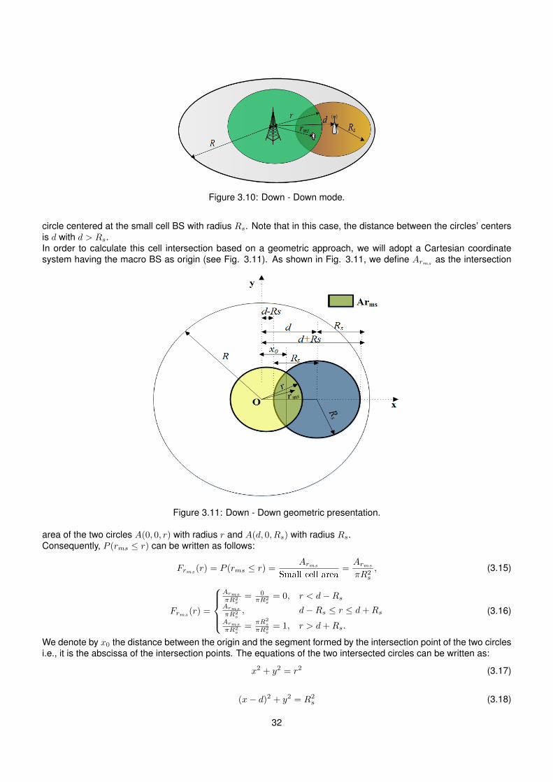
Figure 3.10: Down - Down mode.
circle centered at the small cell BS with radius Rs. Note that in this case, the distance between the circles’ centersis d with d > Rs.In order to calculate this cell intersection based on a geometric approach, we will adopt a Cartesian coordinatesystem having the macro BS as origin (see Fig. 3.11). As shown in Fig. 3.11, we define Arms as the intersection
Figure 3.11: Down - Down geometric presentation.
area of the two circles A(0, 0, r) with radius r and A(d, 0, Rs) with radius Rs.Consequently, P (rms ≤ r) can be written as follows:
Frms(r) = P (rms ≤ r) =Arms
Small cell area=ArmsπR2
s
, (3.15)
Frms(r) =
ArmsπR2
s= 0
πR2s= 0, r < d−Rs
ArmsπR2
s, d−Rs ≤ r ≤ d+Rs
ArmsπR2
s=
πR2s
πR2s= 1, r > d+Rs.
(3.16)
We denote by x0 the distance between the origin and the segment formed by the intersection point of the two circlesi.e., it is the abscissa of the intersection points. The equations of the two intersected circles can be written as:
x2 + y2 = r2 (3.17)
(x− d)2 + y2 = R2s (3.18)
32
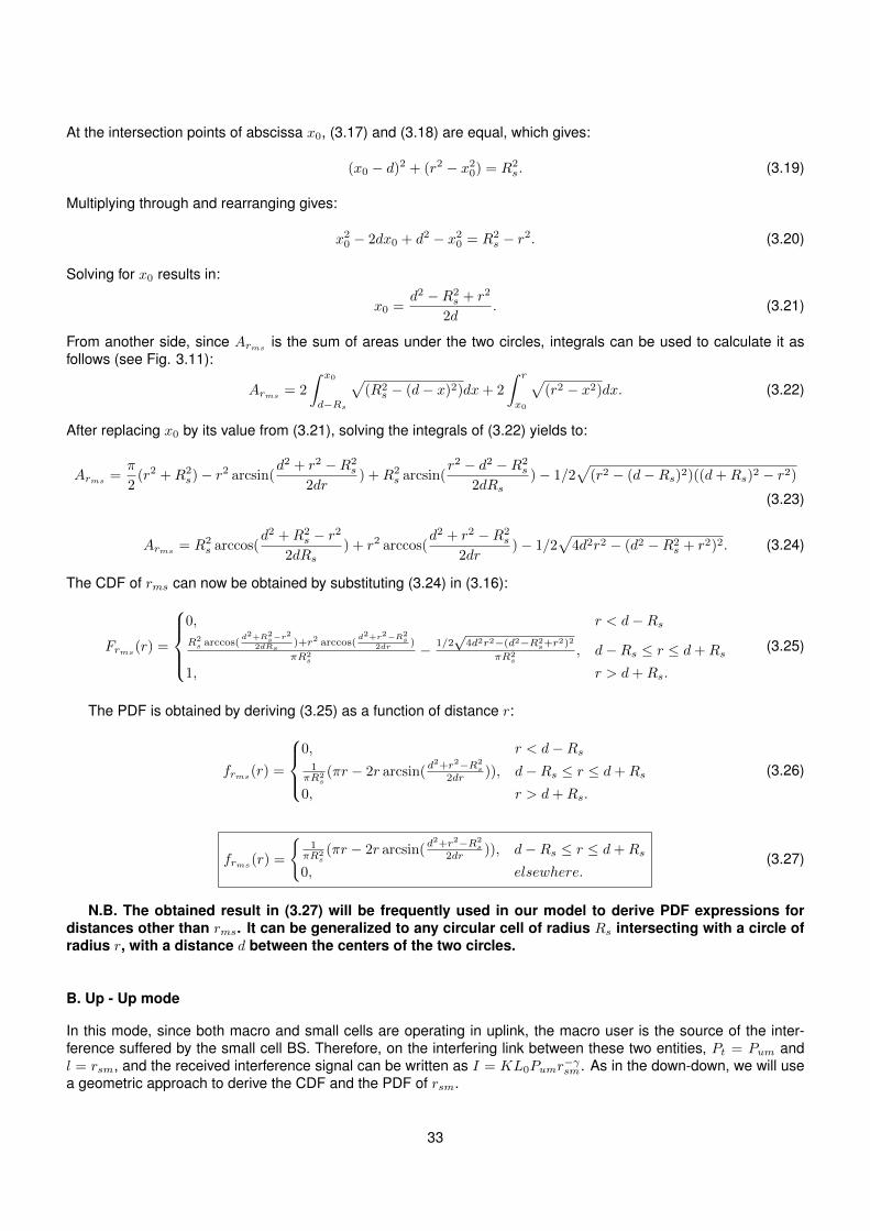
At the intersection points of abscissa x0, (3.17) and (3.18) are equal, which gives:
(x0 − d)2 + (r2 − x20) = R2s. (3.19)
Multiplying through and rearranging gives:
x20 − 2dx0 + d2 − x20 = R2s − r2. (3.20)
Solving for x0 results in:
x0 =d2 −R2
s + r2
2d. (3.21)
From another side, since Arms is the sum of areas under the two circles, integrals can be used to calculate it asfollows (see Fig. 3.11):
Arms = 2
∫ x0
d−Rs
√(R2
s − (d− x)2)dx+ 2
∫ r
x0
√(r2 − x2)dx. (3.22)
After replacing x0 by its value from (3.21), solving the integrals of (3.22) yields to:
Arms =π
2(r2 +R2
s)− r2 arcsin(d2 + r2 −R2
s
2dr) +R2
s arcsin(r2 − d2 −R2
s
2dRs)− 1/2
√(r2 − (d−Rs)2)((d+Rs)2 − r2)
(3.23)
Arms = R2s arccos(
d2 +R2s − r2
2dRs) + r2 arccos(
d2 + r2 −R2s
2dr)− 1/2
√4d2r2 − (d2 −R2
s + r2)2. (3.24)
The CDF of rms can now be obtained by substituting (3.24) in (3.16):
Frms(r) =
0, r < d−RsR2s arccos(
d2+R2s−r
2
2dRs)+r2 arccos(
d2+r2−R2s
2dr )
πR2s
− 1/2√
4d2r2−(d2−R2s+r
2)2
πR2s
, d−Rs ≤ r ≤ d+Rs
1, r > d+Rs.
(3.25)
The PDF is obtained by deriving (3.25) as a function of distance r:
frms(r) =
0, r < d−Rs1
πR2s(πr − 2r arcsin(
d2+r2−R2s
2dr )), d−Rs ≤ r ≤ d+Rs
0, r > d+Rs.
(3.26)
frms(r) =
{1
πR2s(πr − 2r arcsin(
d2+r2−R2s
2dr )), d−Rs ≤ r ≤ d+Rs
0, elsewhere.(3.27)
N.B. The obtained result in (3.27) will be frequently used in our model to derive PDF expressions fordistances other than rms. It can be generalized to any circular cell of radius Rs intersecting with a circle ofradius r, with a distance d between the centers of the two circles.
B. Up - Up mode
In this mode, since both macro and small cells are operating in uplink, the macro user is the source of the inter-ference suffered by the small cell BS. Therefore, on the interfering link between these two entities, Pt = Pum andl = rsm, and the received interference signal can be written as I = KL0Pumr
−γsm. As in the down-down, we will use
a geometric approach to derive the CDF and the PDF of rsm.
33
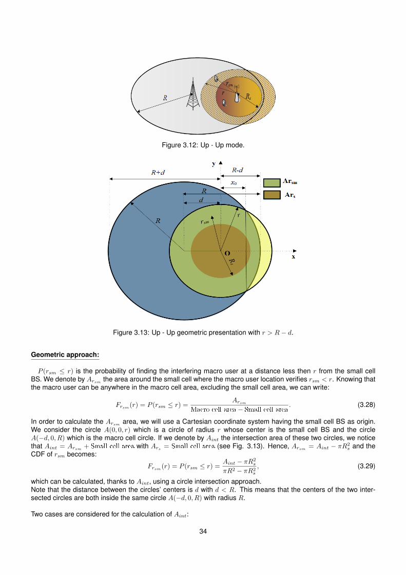
Figure 3.12: Up - Up mode.
Figure 3.13: Up - Up geometric presentation with r > R− d.
Geometric approach:
P (rsm ≤ r) is the probability of finding the interfering macro user at a distance less then r from the small cellBS. We denote by Arsm the area around the small cell where the macro user location verifies rsm < r. Knowing thatthe macro user can be anywhere in the macro cell area, excluding the small cell area, we can write:
Frsm(r) = P (rsm ≤ r) =Arsm
Macro cell area− Small cell area. (3.28)
In order to calculate the Arsm area, we will use a Cartesian coordinate system having the small cell BS as origin.We consider the circle A(0, 0, r) which is a circle of radius r whose center is the small cell BS and the circleA(−d, 0, R) which is the macro cell circle. If we denote by Aint the intersection area of these two circles, we noticethat Aint = Arsm + Small cell area with Ars = Small cell area (see Fig. 3.13). Hence, Arsm = Aint − πR2
s and theCDF of rsm becomes:
Frsm(r) = P (rsm ≤ r) =Aint − πR2
s
πR2 − πR2s
, (3.29)
which can be calculated, thanks to Aint, using a circle intersection approach.Note that the distance between the circles’ centers is d with d < R. This means that the centers of the two inter-sected circles are both inside the same circle A(−d, 0, R) with radius R.
Two cases are considered for the calculation of Aint:
34
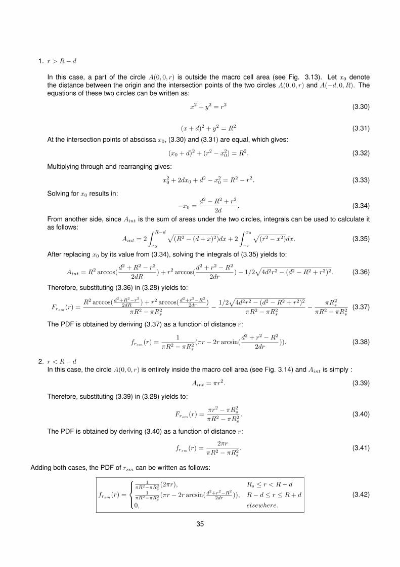
1. r > R− d
In this case, a part of the circle A(0, 0, r) is outside the macro cell area (see Fig. 3.13). Let x0 denotethe distance between the origin and the intersection points of the two circles A(0, 0, r) and A(−d, 0, R). Theequations of these two circles can be written as:
x2 + y2 = r2 (3.30)
(x+ d)2 + y2 = R2 (3.31)
At the intersection points of abscissa x0, (3.30) and (3.31) are equal, which gives:
(x0 + d)2 + (r2 − x20) = R2. (3.32)
Multiplying through and rearranging gives:
x20 + 2dx0 + d2 − x20 = R2 − r2. (3.33)
Solving for x0 results in:
−x0 =d2 −R2 + r2
2d. (3.34)
From another side, since Aint is the sum of areas under the two circles, integrals can be used to calculate itas follows:
Aint = 2
∫ R−d
x0
√(R2 − (d+ x)2)dx+ 2
∫ x0
−r
√(r2 − x2)dx. (3.35)
After replacing x0 by its value from (3.34), solving the integrals of (3.35) yields to:
Aint = R2 arccos(d2 +R2 − r2
2dR) + r2 arccos(
d2 + r2 −R2
2dr)− 1/2
√4d2r2 − (d2 −R2 + r2)2. (3.36)
Therefore, substituting (3.36) in (3.28) yields to:
Frsm(r) =R2 arccos(d
2+R2−r22dR ) + r2 arccos(d
2+r2−R2
2dr )
πR2 − πR2s
−1/2√
4d2r2 − (d2 −R2 + r2)2
πR2 − πR2s
− πR2s
πR2 − πR2s
(3.37)
The PDF is obtained by deriving (3.37) as a function of distance r:
frsm(r) =1
πR2 − πR2s
(πr − 2r arcsin(d2 + r2 −R2
2dr)). (3.38)
2. r < R− dIn this case, the circle A(0, 0, r) is entirely inside the macro cell area (see Fig. 3.14) and Aint is simply :
Aint = πr2. (3.39)
Therefore, substituting (3.39) in (3.28) yields to:
Frsm(r) =πr2 − πR2
s
πR2 − πR2s
. (3.40)
The PDF is obtained by deriving (3.40) as a function of distance r:
frsm(r) =2πr
πR2 − πR2s
. (3.41)
Adding both cases, the PDF of rsm can be written as follows:
frsm(r) =
1
πR2−πR2s(2πr), Rs ≤ r < R− d
1πR2−πR2
s(πr − 2r arcsin(d
2+r2−R2
2dr )), R− d ≤ r ≤ R+ d
0, elsewhere.
(3.42)
35
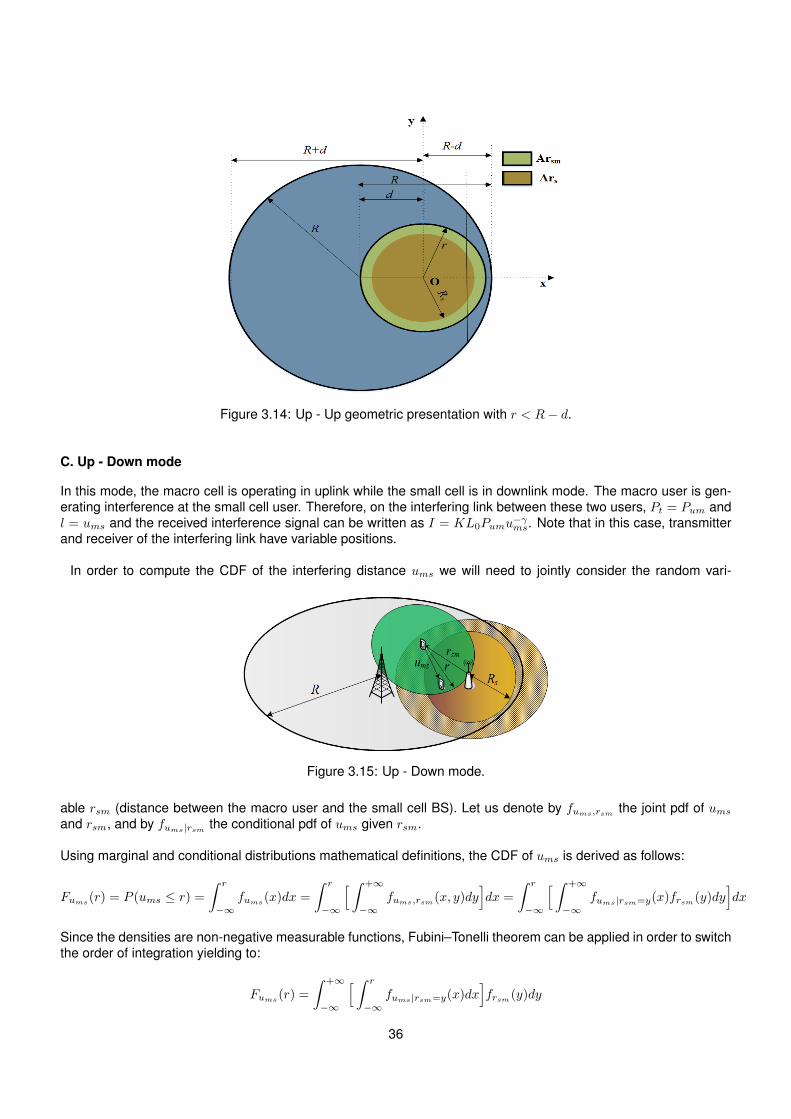
Figure 3.14: Up - Up geometric presentation with r < R− d.
C. Up - Down mode
In this mode, the macro cell is operating in uplink while the small cell is in downlink mode. The macro user is gen-erating interference at the small cell user. Therefore, on the interfering link between these two users, Pt = Pum andl = ums and the received interference signal can be written as I = KL0Pumu
−γms. Note that in this case, transmitter
and receiver of the interfering link have variable positions.
In order to compute the CDF of the interfering distance ums we will need to jointly consider the random vari-
Figure 3.15: Up - Down mode.
able rsm (distance between the macro user and the small cell BS). Let us denote by fums,rsm the joint pdf of umsand rsm, and by fums|rsm the conditional pdf of ums given rsm.
Using marginal and conditional distributions mathematical definitions, the CDF of ums is derived as follows:
Fums(r) = P (ums ≤ r) =∫ r
−∞fums(x)dx =
∫ r
−∞
[ ∫ +∞
−∞fums,rsm(x, y)dy
]dx =
∫ r
−∞
[ ∫ +∞
−∞fums|rsm=y(x)frsm(y)dy
]dx
Since the densities are non-negative measurable functions, Fubini–Tonelli theorem can be applied in order to switchthe order of integration yielding to:
Fums(r) =
∫ +∞
−∞
[ ∫ r
−∞fums|rsm=y(x)dx
]frsm(y)dy
36
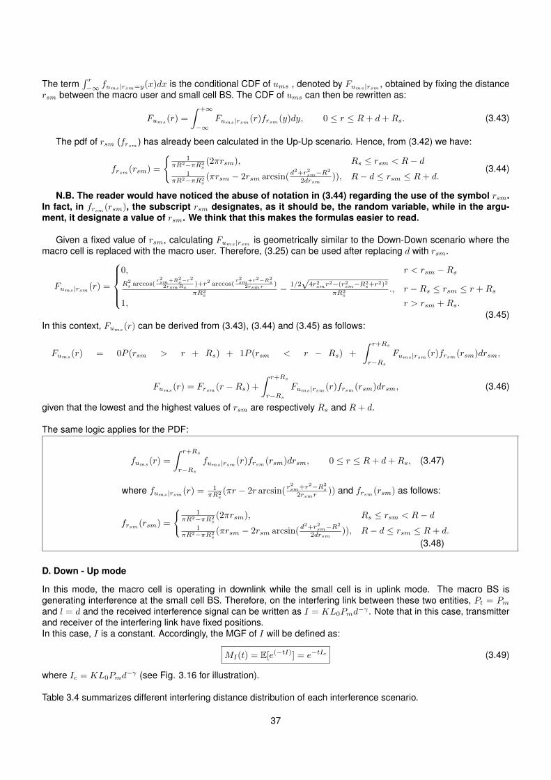
The term∫ r−∞ fums|rsm=y(x)dx is the conditional CDF of ums , denoted by Fums|rsm , obtained by fixing the distance
rsm between the macro user and small cell BS. The CDF of ums can then be rewritten as:
Fums(r) =
∫ +∞
−∞Fums|rsm(r)frsm(y)dy, 0 ≤ r ≤ R+ d+Rs. (3.43)
The pdf of rsm (frsm ) has already been calculated in the Up-Up scenario. Hence, from (3.42) we have:
frsm(rsm) =
{1
πR2−πR2s(2πrsm), Rs ≤ rsm < R− d
1πR2−πR2
s(πrsm − 2rsm arcsin(
d2+r2sm−R2
2drsm)), R− d ≤ rsm ≤ R+ d.
(3.44)
N.B. The reader would have noticed the abuse of notation in (3.44) regarding the use of the symbol rsm.In fact, in frsm(rsm), the subscript rsm designates, as it should be, the random variable, while in the argu-ment, it designate a value of rsm. We think that this makes the formulas easier to read.
Given a fixed value of rsm, calculating Fums|rsm is geometrically similar to the Down-Down scenario where themacro cell is replaced with the macro user. Therefore, (3.25) can be used after replacing d with rsm.
Fums|rsm(r) =
0, r < rsm −RsR2s arccos(
r2sm+R2s−r
2
2rsmRs)+r2 arccos(
r2sm+r2−R2s
2rsmr)
πR2s
− 1/2√
4r2smr2−(r2sm−R2
s+r2)2
πR2s
., r −Rs ≤ rsm ≤ r +Rs
1, r > rsm +Rs.
(3.45)In this context, Fums(r) can be derived from (3.43), (3.44) and (3.45) as follows:
Fums(r) = 0P (rsm > r + Rs) + 1P (rsm < r − Rs) +
∫ r+Rs
r−RsFums|rsm(r)frsm(rsm)drsm,
Fums(r) = Frsm(r −Rs) +∫ r+Rs
r−RsFums|rsm(r)frsm(rsm)drsm, (3.46)
given that the lowest and the highest values of rsm are respectively Rs and R+ d.
The same logic applies for the PDF:
fums(r) =
∫ r+Rs
r−Rsfums|rsm(r)frsm(rsm)drsm, 0 ≤ r ≤ R+ d+Rs, (3.47)
where fums|rsm(r) =1
πR2s(πr − 2r arcsin(
r2sm+r2−R2s
2rsmr)) and frsm(rsm) as follows:
frsm(rsm) =
{1
πR2−πR2s(2πrsm), Rs ≤ rsm < R− d
1πR2−πR2
s(πrsm − 2rsm arcsin(
d2+r2sm−R2
2drsm)), R− d ≤ rsm ≤ R+ d.
(3.48)
D. Down - Up mode
In this mode, the macro cell is operating in downlink while the small cell is in uplink mode. The macro BS isgenerating interference at the small cell BS. Therefore, on the interfering link between these two entities, Pt = Pmand l = d and the received interference signal can be written as I = KL0Pmd
−γ . Note that in this case, transmitterand receiver of the interfering link have fixed positions.In this case, I is a constant. Accordingly, the MGF of I will be defined as:
MI(t) = E[e(−tI)] = e−tIc (3.49)
where Ic = KL0Pmd−γ (see Fig. 3.16 for illustration).
Table 3.4 summarizes different interfering distance distribution of each interference scenario.
37
Figure 3.16: Down - Up mode.
Macro Small cell Scenario Interfering Distance Distribution
Down Down BS-MS frms(r) =1
πR2s(πr − 2r arcsin(
d2 + r2 −R2s
2dr)), d−Rs ≤ r ≤ d+Rs
Up Up MS-BS frsm(r) =
1
πR2−πR2s(2πr), Rs ≤ r < R− d
1πR2−πR2
s(πr − 2r arcsin( d
2+r2−R2
2dr )), R− d ≤ r ≤ R+ d
Up Down MS-MS
fums(r) =
∫ r+Rs
r−Rsfums|rsm(r)frsm(rsm)drsm, 0 ≤ r ≤ R+ d+Rs,
fums|rsm(r) =1
πR2s(πr − 2r arcsin(
r2sm + r2 −R2s
2rsmr))
frsm(rsm) =
1
πR2−πR2s(2πrsm), Rs ≤ rsm < R− d
1πR2−πR2
s(πrsm − 2rsm arcsin(
d2+r2sm−R2
2drsm)), R− d ≤ rsm ≤ R+ d
Down Up BS-BS d = constant
Table 3.4: Summary of interfering distances distributions.
3.3.3 Capacity Analysis in Single Small Cell Scenario
The average user capacity per unit bandwidth i.e. the spectral efficiency at the reference small cell, is defined asthe achievable average rate of the link to the allocated bandwidth (B), expressed mathematically by the modifiedShannon’s formula as:
Cs = E[B ln(1 + S
I+σ2 )
B
]= E
[ln(1 +
S
I + σ2)], (3.50)
with σ2 the thermal noise power variance.
The latter can be calculated using the lemma proposed in [112] as follows:
Cs = E[ln(1 +S
I + σ2)] =
∫ ∞0
MI(t)−MS(t)MI(t)
te−(σ
2)tdt =
∫ ∞0
MI(t)−MS(t)MI(t)
te−ate−(σ
2+a)tdt, (3.51)
38
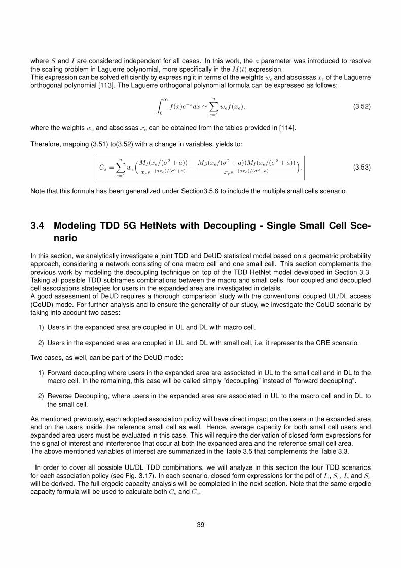
where S and I are considered independent for all cases. In this work, the a parameter was introduced to resolvethe scaling problem in Laguerre polynomial, more specifically in the M(t) expression.This expression can be solved efficiently by expressing it in terms of the weights we and abscissas xe of the Laguerreorthogonal polynomial [113]. The Laguerre orthogonal polynomial formula can be expressed as follows:∫ ∞
0
f(x)e−xdx 'n∑e=1
wef(xe), (3.52)
where the weights we and abscissas xe can be obtained from the tables provided in [114].
Therefore, mapping (3.51) to(3.52) with a change in variables, yields to:
Cs =
n∑e=1
we
(MI(xe/(σ2 + a))
xee−(axe)/(σ2+a)
− MS(xe/(σ2 + a))MI(xe/(σ
2 + a))
xee−(axe)/(σ2+a)
). (3.53)
Note that this formula has been generalized under Section3.5.6 to include the multiple small cells scenario.
3.4 Modeling TDD 5G HetNets with Decoupling - Single Small Cell Sce-nario
In this section, we analytically investigate a joint TDD and DeUD statistical model based on a geometric probabilityapproach, considering a network consisting of one macro cell and one small cell. This section complements theprevious work by modeling the decoupling technique on top of the TDD HetNet model developed in Section 3.3.Taking all possible TDD subframes combinations between the macro and small cells, four coupled and decoupledcell associations strategies for users in the expanded area are investigated in details.A good assessment of DeUD requires a thorough comparison study with the conventional coupled UL/DL access(CoUD) mode. For further analysis and to ensure the generality of our study, we investigate the CoUD scenario bytaking into account two cases:
1) Users in the expanded area are coupled in UL and DL with macro cell.
2) Users in the expanded area are coupled in UL and DL with small cell, i.e. it represents the CRE scenario.
Two cases, as well, can be part of the DeUD mode:
1) Forward decoupling where users in the expanded area are associated in UL to the small cell and in DL to themacro cell. In the remaining, this case will be called simply "decoupling" instead of "forward decoupling".
2) Reverse Decoupling, where users in the expanded area are associated in UL to the macro cell and in DL tothe small cell.
As mentioned previously, each adopted association policy will have direct impact on the users in the expanded areaand on the users inside the reference small cell as well. Hence, average capacity for both small cell users andexpanded area users must be evaluated in this case. This will require the derivation of closed form expressions forthe signal of interest and interference that occur at both the expanded area and the reference small cell area.The above mentioned variables of interest are summarized in the Table 3.5 that complements the Table 3.3.
In order to cover all possible UL/DL TDD combinations, we will analyze in this section the four TDD scenariosfor each association policy (see Fig. 3.17). In each scenario, closed form expressions for the pdf of Ie, Se, Is and Sswill be derived. The full ergodic capacity analysis will be completed in the next section. Note that the same ergodiccapacity formula will be used to calculate both Cs and Ce.
39
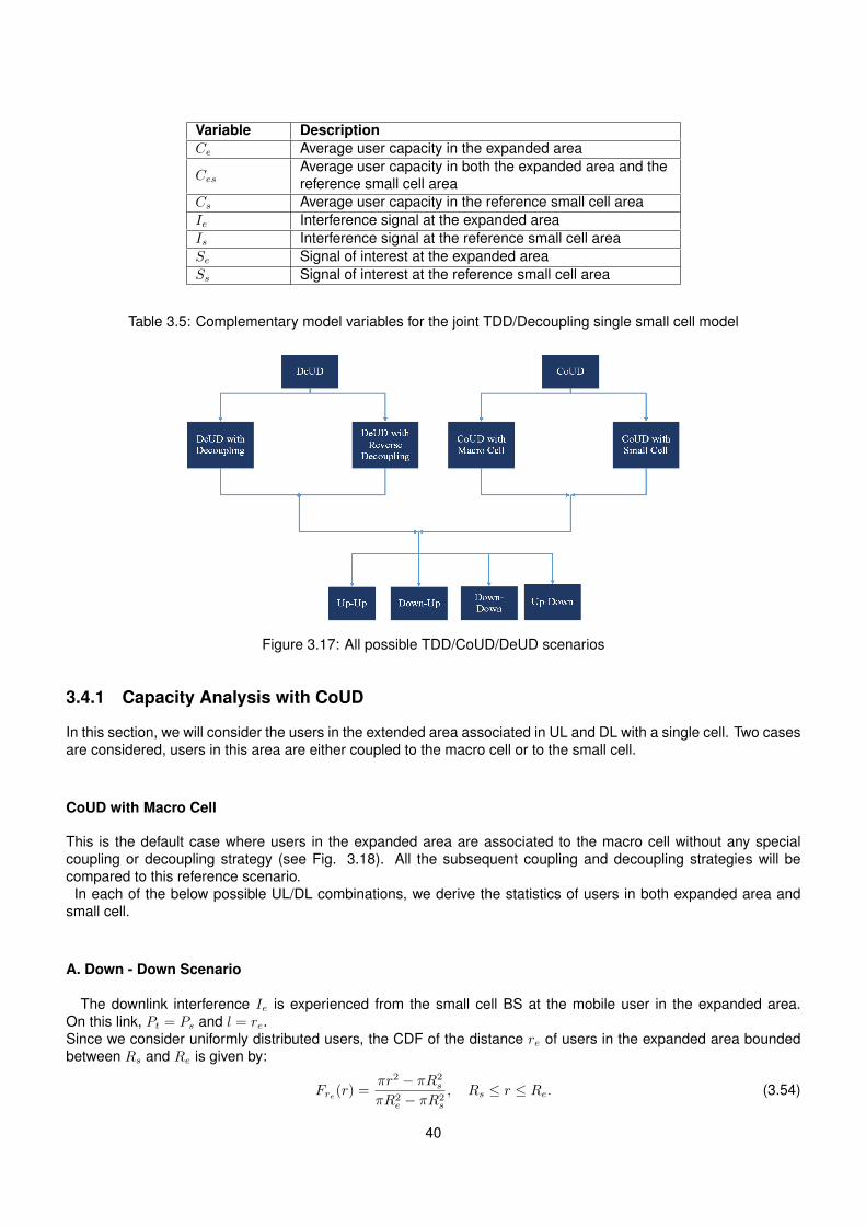
Variable DescriptionCe Average user capacity in the expanded area
CesAverage user capacity in both the expanded area and thereference small cell area
Cs Average user capacity in the reference small cell areaIe Interference signal at the expanded areaIs Interference signal at the reference small cell areaSe Signal of interest at the expanded areaSs Signal of interest at the reference small cell area
Table 3.5: Complementary model variables for the joint TDD/Decoupling single small cell model
Figure 3.17: All possible TDD/CoUD/DeUD scenarios
3.4.1 Capacity Analysis with CoUD
In this section, we will consider the users in the extended area associated in UL and DL with a single cell. Two casesare considered, users in this area are either coupled to the macro cell or to the small cell.
CoUD with Macro Cell
This is the default case where users in the expanded area are associated to the macro cell without any specialcoupling or decoupling strategy (see Fig. 3.18). All the subsequent coupling and decoupling strategies will becompared to this reference scenario.
In each of the below possible UL/DL combinations, we derive the statistics of users in both expanded area andsmall cell.
A. Down - Down Scenario
The downlink interference Ie is experienced from the small cell BS at the mobile user in the expanded area.On this link, Pt = Ps and l = re.Since we consider uniformly distributed users, the CDF of the distance re of users in the expanded area boundedbetween Rs and Re is given by:
Fre(r) =πr2 − πR2
s
πR2e − πR2
s
, Rs ≤ r ≤ Re. (3.54)
40
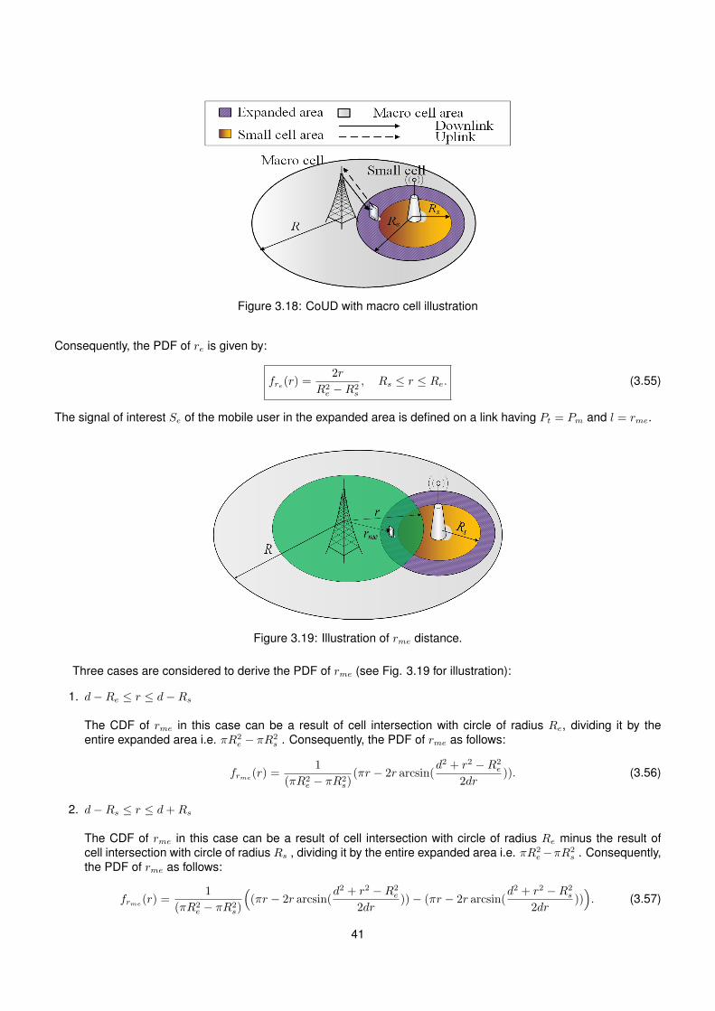
Figure 3.18: CoUD with macro cell illustration
Consequently, the PDF of re is given by:
fre(r) =2r
R2e −R2
s
, Rs ≤ r ≤ Re. (3.55)
The signal of interest Se of the mobile user in the expanded area is defined on a link having Pt = Pm and l = rme.
Figure 3.19: Illustration of rme distance.
Three cases are considered to derive the PDF of rme (see Fig. 3.19 for illustration):
1. d−Re ≤ r ≤ d−Rs
The CDF of rme in this case can be a result of cell intersection with circle of radius Re, dividing it by theentire expanded area i.e. πR2
e − πR2s . Consequently, the PDF of rme as follows:
frme(r) =1
(πR2e − πR2
s)(πr − 2r arcsin(
d2 + r2 −R2e
2dr)). (3.56)
2. d−Rs ≤ r ≤ d+Rs
The CDF of rme in this case can be a result of cell intersection with circle of radius Re minus the result ofcell intersection with circle of radius Rs , dividing it by the entire expanded area i.e. πR2
e−πR2s . Consequently,
the PDF of rme as follows:
frme(r) =1
(πR2e − πR2
s)
((πr − 2r arcsin(
d2 + r2 −R2e
2dr))− (πr − 2r arcsin(
d2 + r2 −R2s
2dr))). (3.57)
41
3. d+Rs ≤ r ≤ d+Re
The CDF of rme in this case is defined as:
Frme(r) = F3(r)−πR2
s
(πR2e − πR2
s), (3.58)
with F3(r) a CDF that results from a cell intersection with a circle of radius Re .By applying the derivative of Frme(r) and since the second term is a constant, the PDF frme(r) will be:
frme(r) = f3(r) =1
(πR2e − πR2
s)(πr − 2r arcsin(
d2 + r2 −R2e
2dr)), (3.59)
with f3(r) defined as the derivative of F3(r).
Adding the three cases, the probability density function (PDF) of rme can be written as:
frme(r) =
1
(πR2e−πR2
s)(πr − 2r arcsin( d
2+r2−R2e
2dr)), d−Re ≤ r ≤ d−Rs
1(πR2
e−πR2s)
((πr − 2r arcsin( d
2+r2−R2e
2dr))− (πr − 2r arcsin( d
2+r2−R2s
2dr))), d−Rs ≤ r ≤ d+Rs
1(πR2
e−πR2s)(πr − 2r arcsin( d
2+r2−R2e
2dr)), d+Rs ≤ r ≤ d+Re.
(3.60)
As for the statistics related to the small cell users, the downlink interference Is is experienced from the macroBS at the small cell users. On this link, Pt = Pm and l = rs. Based on the expression (3.27) derived in the previoussection, the PDF of rms can be obtained as a result of cell intersection with circle of radius Rs:
frms(r) =1
πR2s
(πr − 2r arcsin(d2 + r2 −R2
s
2dr)). (3.61)
The signal of interest Ss of the small cell user is defined on a link having Pt = Ps and l = rs.Since we consider uniformly distributed users, the distribution of the distance rs of a small cell user is given by:
frs(r) =2r
R2s
, 0 ≤ r ≤ Rs. (3.62)
Note that the same distribution of rs will be applicable for all coming scenarios.
B. Up - Down Scenario
The uplink interference Ie is experienced from the small cell BS at the macro BS. On this link, Pt = Ps andl = d.The uplink desired signal Se of the mobile user in the expanded area is defined on a link having Pt = Pum andl = rme.Repeating the same analysis as in (3.60), the PDF of rme can be written as:
frme(r) =
1
(πR2e−πR2
s)(πr − 2r arcsin( d
2+r2−R2e
2dr)), d−Re ≤ r ≤ d−Rs
1(πR2
e−πR2s)
((πr − 2r arcsin(
d2+r2−R2e
2dr))− (πr − 2r arcsin(
d2+r2−R2s
2dr))), d−Rs ≤ r ≤ d+Rs
1(πR2
e−πR2s)(πr − 2r arcsin( d
2+r2−R2e
2dr)), d+Rs ≤ r ≤ d+Re.
(3.63)
As for the statistics related to the small cell users, the downlink interference Is is experienced from the macrocell user at the small cell user. On this link, Pt = Pum and l = ums.Based on the expression (3.47) derived in the Up - Down scenario, the PDF of ums can be written as follows:
fums(r) =
∫ r+Rs
r−Rsfums|rsm(r)frsm(rsm)drsm, 0 ≤ r ≤ R+ d+Rs, (3.64)
where fums|rsm(r) =1
πR2s(πr − 2r arcsin(
r2sm+r2−R2s
2rsmr)) and frsm(rsm) defined as follows:
frsm(rsm) =
{1
πR2−πR2s(2πrsm), Rs ≤ rsm < R− d
1πR2−πR2
s(πrsm − 2rsm arcsin( d
2+r2sm−R2
2drsm)), R− d ≤ rsm ≤ R+ d.
(3.65)
The signal of interest Ss of the small cell user is defined on a link having Pt = Ps and l = rs.
42
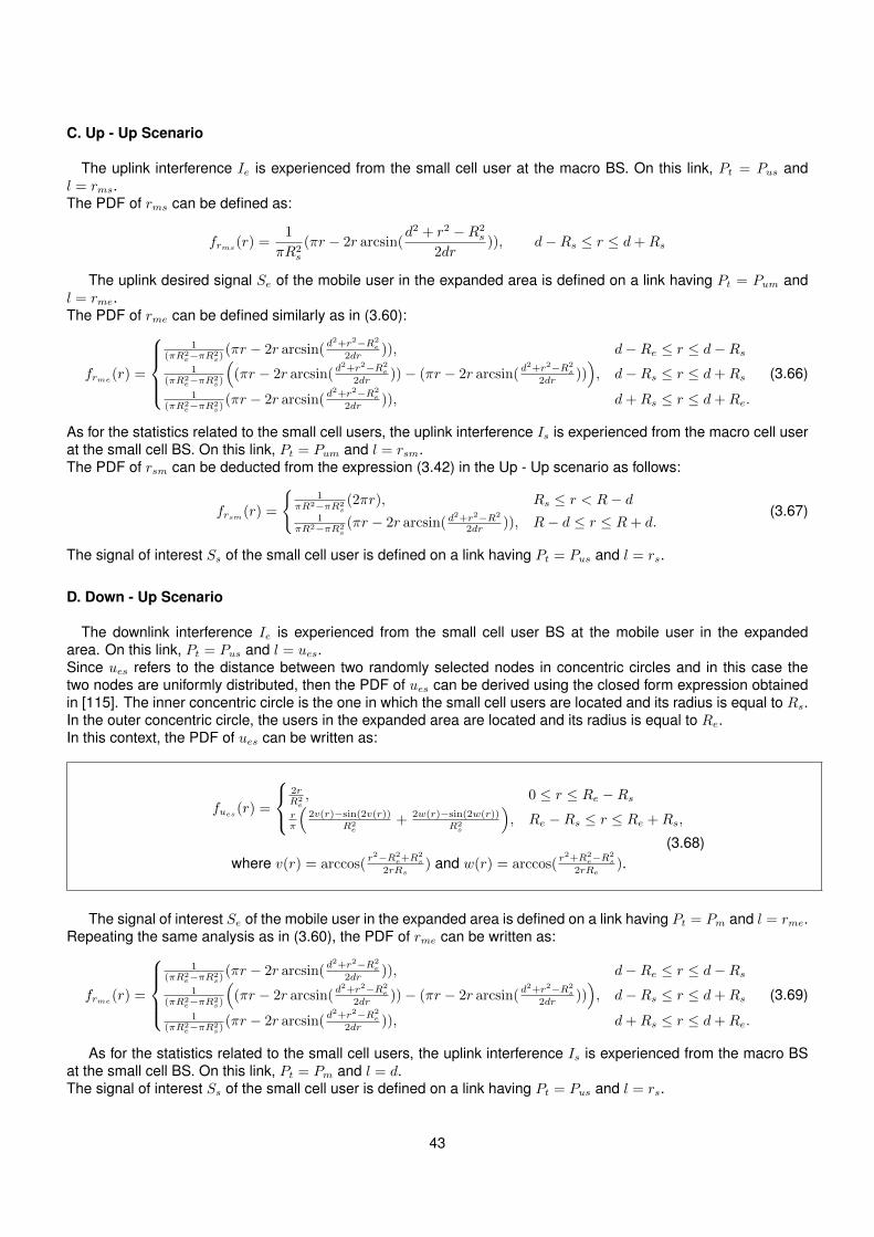
C. Up - Up Scenario
The uplink interference Ie is experienced from the small cell user at the macro BS. On this link, Pt = Pus andl = rms.The PDF of rms can be defined as:
frms(r) =1
πR2s
(πr − 2r arcsin(d2 + r2 −R2
s
2dr)), d−Rs ≤ r ≤ d+Rs
The uplink desired signal Se of the mobile user in the expanded area is defined on a link having Pt = Pum andl = rme.The PDF of rme can be defined similarly as in (3.60):
frme(r) =
1
(πR2e−πR2
s)(πr − 2r arcsin( d
2+r2−R2e
2dr)), d−Re ≤ r ≤ d−Rs
1(πR2
e−πR2s)
((πr − 2r arcsin( d
2+r2−R2e
2dr))− (πr − 2r arcsin( d
2+r2−R2s
2dr))), d−Rs ≤ r ≤ d+Rs
1(πR2
e−πR2s)(πr − 2r arcsin(
d2+r2−R2e
2dr)), d+Rs ≤ r ≤ d+Re.
(3.66)
As for the statistics related to the small cell users, the uplink interference Is is experienced from the macro cell userat the small cell BS. On this link, Pt = Pum and l = rsm.The PDF of rsm can be deducted from the expression (3.42) in the Up - Up scenario as follows:
frsm(r) =
{1
πR2−πR2s(2πr), Rs ≤ r < R− d
1πR2−πR2
s(πr − 2r arcsin( d
2+r2−R2
2dr)), R− d ≤ r ≤ R+ d.
(3.67)
The signal of interest Ss of the small cell user is defined on a link having Pt = Pus and l = rs.
D. Down - Up Scenario
The downlink interference Ie is experienced from the small cell user BS at the mobile user in the expandedarea. On this link, Pt = Pus and l = ues.Since ues refers to the distance between two randomly selected nodes in concentric circles and in this case thetwo nodes are uniformly distributed, then the PDF of ues can be derived using the closed form expression obtainedin [115]. The inner concentric circle is the one in which the small cell users are located and its radius is equal to Rs.In the outer concentric circle, the users in the expanded area are located and its radius is equal to Re.In this context, the PDF of ues can be written as:
fues(r) =
2rR2e, 0 ≤ r ≤ Re −Rs
rπ
(2v(r)−sin(2v(r))
R2e
+ 2w(r)−sin(2w(r))R2s
), Re −Rs ≤ r ≤ Re +Rs,
(3.68)where v(r) = arccos(
r2−R2e+R
2s
2rRs) and w(r) = arccos(
r2+R2e−R
2s
2rRe).
The signal of interest Se of the mobile user in the expanded area is defined on a link having Pt = Pm and l = rme.Repeating the same analysis as in (3.60), the PDF of rme can be written as:
frme(r) =
1
(πR2e−πR2
s)(πr − 2r arcsin( d
2+r2−R2e
2dr)), d−Re ≤ r ≤ d−Rs
1(πR2
e−πR2s)
((πr − 2r arcsin( d
2+r2−R2e
2dr))− (πr − 2r arcsin( d
2+r2−R2s
2dr))), d−Rs ≤ r ≤ d+Rs
1(πR2
e−πR2s)(πr − 2r arcsin( d
2+r2−R2e
2dr)), d+Rs ≤ r ≤ d+Re.
(3.69)
As for the statistics related to the small cell users, the uplink interference Is is experienced from the macro BSat the small cell BS. On this link, Pt = Pm and l = d.The signal of interest Ss of the small cell user is defined on a link having Pt = Pus and l = rs.
43
CoUD with Small Cell or CRE Scenario
A major issue in HetNet planning is to ensure that the small cells actually serve enough users. One way to do that isto increase the area served by the small cell, which can be done through the use of a positive cell selection offset tothe received power of the small cell. Extending the coverage of a cell by means of connecting a UE to a cell whosesignal is weaker than the strongest detected cell signal, is referred to as cell range extension (CRE) [116]. Figure3.20 illustrates the CRE concept, where users in the expanded area are associated in both UL and DL directionswith the small cell.
Figure 3.20: CRE illustration
In each of the following scenario under CRE, we will derive the statistics of users in the expanded area apart, inaddition to the the small users’ figures.
A. Down - Down Scenario
The downlink interference Ie is experienced from the macro BS at the mobile user in the expanded area. Onthis link, Pt = Pm and l = rme.Repeating the same analysis as in (3.60), the PDF of rme can be written as:
frme(r) =
1
(πR2e−πR2
s)(πr − 2r arcsin(
d2+r2−R2e
2dr)), d−Re ≤ r ≤ d−Rs
1(πR2
e−πR2s)
((πr − 2r arcsin( d
2+r2−R2e
2dr))− (πr − 2r arcsin( d
2+r2−R2s
2dr))), d−Rs ≤ r ≤ d+Rs
1(πR2
e−πR2s)(πr − 2r arcsin( d
2+r2−R2e
2dr)), d+Rs ≤ r ≤ d+Re.
(3.70)
The signal of interest Se of the mobile user in the expanded area is defined on a link having Pt = Ps and l = re.The distribution of re is given by (3.55).
As for the statistics related to the small cell users, the downlink interference Is is experienced from the macroBS at the small cell users. On this link, Pt = Pm and l = rms.The PDF of rms can be obtained as a result of cell intersection with circle of radius Rs:
frms(r) =1
πR2s
(πr − 2r arcsin(d2 + r2 −R2
s
2dr)), d−Rs ≤ r ≤ d+Rs. (3.71)
The signal of interest Ss of the small cell user is defined on a link having Pt = Ps and l = rs.
B. Up - Down Scenario
The downlink interference Ie is experienced from the macro cell user at the small cell user that is located in-side the area bounded by Re. On this link, Pt = Pum and l = ums.The PDF of ums is given by replacing Rs with Re in (3.64):
fums(r) =
∫ r+Re
r−Refums|rsm(r)frsm(rsm)drsm, 0 ≤ r ≤ R+ d+Re, (3.72)
44
where fums|rsm(r) =1
πR2e(πr − 2r arcsin(
r2sm+r2−R2e
2rsmr)) and frsm(rsm) formulated as:
frsm(rsm) =
{1
πR2−πR2e(2πrsm), Re ≤ rsm < R− d
1πR2−πR2
e(πrsm − 2rsm arcsin(
d2+r2sm−R2
2drsm)), R− d ≤ rsm ≤ R+ d
(3.73)
The signal of interest Se of the mobile user in the expanded area is defined on a link having Pt = Ps and l = re.The distribution of re is given by (3.55).
As for the statistics related to the small cell users, the downlink interference Is is experienced from the macrocell user at the small cell user that is located inside the area bounded by Re. On this link, Pt = Pum and l = ums.The distribution of ums is given by (3.72). For simplicity, we considered the same distance ums to measure thedistance from the macro user to either the small cell user or the user in the expanded area. This approximation isvalid due to the notably smaller size of small cells comparing to the macro cell. The signal of interest Ss of the smallcell user is defined on a link having Pt = Ps and l = rs.
C. Up - Up Scenario
The uplink interference Ie is experienced from the macro cell user that is located outside the area boundedby Re at the small cell BS. On this link, Pt = Pum and l = rsm.The PDF of rsm is derived as in (3.73) where Re is replacing Rs:
frsm(r) =
{1
πR2−πR2e(2πr), Re ≤ r < R− d
1πR2−πR2
e(πr − 2r arcsin( d
2+r2−R2
2dr)), R− d ≤ r ≤ R+ d.
(3.74)
The uplink desired signal Se of the mobile user in the expanded area is defined on a link having Pt = Pus and l = re.The distribution of re is given by (3.55).
As for the statistics related to the small cell users, the uplink interference Is is defined on a link having Pt = Pumand l = rsm.Same distance rsm as in (3.74) will be studied for simplicity. The accuracy of this approximation will be validated inthe next chapter using Monte-Carlo simulations.The signal of interest Ss of the small cell user is defined on a link having Pt = Pus and l = rs.
D. Down - Up Scenario
The uplink interference Ie is experienced from the macro cell BS at the small cell BS. On this link, Pt = Pmand l = d.The signal of interest Se of the mobile user in the expanded area is defined on a link having Pt = Pus and l = re.The distribution of re is given by (3.55).
As for the statistics related to the small cell users, they can be modeled by replacing re with rs in the expressionsderived for the mobile users in the expanded area under this same scenario.
3.4.2 Capacity Analysis with DeUD
In this section, we will consider the users in the extended area simultaneously connected to two cells, one for thedownlink and one for the uplink. Two cases are considered, decoupling access or reverse decoupling access.
DeUD with Decoupling
Figure 3.21 illustrates the DeUD with decoupling case, where users in the expanded area are associated in UL tothe small cell and in DL to the macro cell.
45
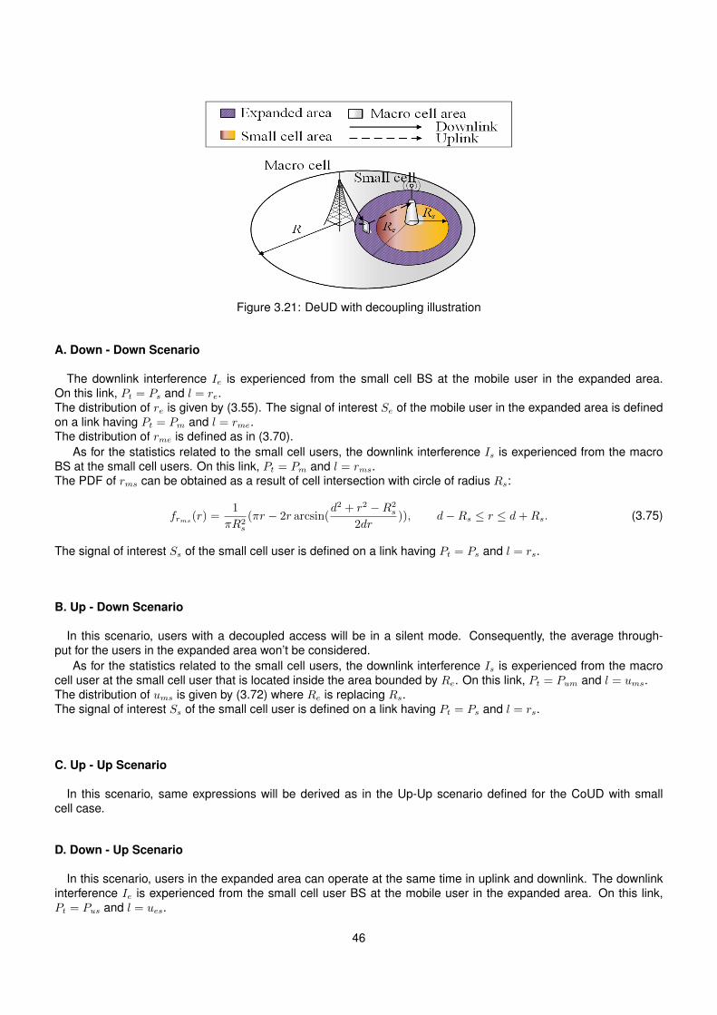
Figure 3.21: DeUD with decoupling illustration
A. Down - Down Scenario
The downlink interference Ie is experienced from the small cell BS at the mobile user in the expanded area.On this link, Pt = Ps and l = re.The distribution of re is given by (3.55). The signal of interest Se of the mobile user in the expanded area is definedon a link having Pt = Pm and l = rme.The distribution of rme is defined as in (3.70).
As for the statistics related to the small cell users, the downlink interference Is is experienced from the macroBS at the small cell users. On this link, Pt = Pm and l = rms.The PDF of rms can be obtained as a result of cell intersection with circle of radius Rs:
frms(r) =1
πR2s
(πr − 2r arcsin(d2 + r2 −R2
s
2dr)), d−Rs ≤ r ≤ d+Rs. (3.75)
The signal of interest Ss of the small cell user is defined on a link having Pt = Ps and l = rs.
B. Up - Down Scenario
In this scenario, users with a decoupled access will be in a silent mode. Consequently, the average through-put for the users in the expanded area won’t be considered.
As for the statistics related to the small cell users, the downlink interference Is is experienced from the macrocell user at the small cell user that is located inside the area bounded by Re. On this link, Pt = Pum and l = ums.The distribution of ums is given by (3.72) where Re is replacing Rs.The signal of interest Ss of the small cell user is defined on a link having Pt = Ps and l = rs.
C. Up - Up Scenario
In this scenario, same expressions will be derived as in the Up-Up scenario defined for the CoUD with smallcell case.
D. Down - Up Scenario
In this scenario, users in the expanded area can operate at the same time in uplink and downlink. The downlinkinterference Ie is experienced from the small cell user BS at the mobile user in the expanded area. On this link,Pt = Pus and l = ues.
46
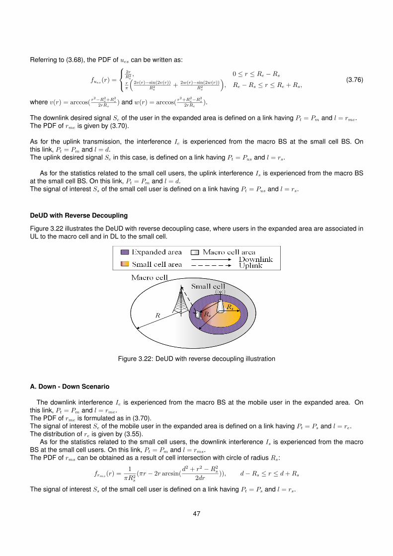
Referring to (3.68), the PDF of ues can be written as:
fues(r) =
2rR2e, 0 ≤ r ≤ Re −Rs
rπ
(2v(r)−sin(2v(r))
R2e
+ 2w(r)−sin(2w(r))R2s
), Re −Rs ≤ r ≤ Re +Rs,
(3.76)
where v(r) = arccos( r2−R2
e+R2s
2rRs) and w(r) = arccos( r
2+R2e−R
2s
2rRe).
The downlink desired signal Se of the user in the expanded area is defined on a link having Pt = Pm and l = rme.The PDF of rme is given by (3.70).
As for the uplink transmission, the interference Ie is experienced from the macro BS at the small cell BS. Onthis link, Pt = Pm and l = d.The uplink desired signal Se in this case, is defined on a link having Pt = Pus and l = rs.
As for the statistics related to the small cell users, the uplink interference Is is experienced from the macro BSat the small cell BS. On this link, Pt = Pm and l = d.The signal of interest Ss of the small cell user is defined on a link having Pt = Pus and l = rs.
DeUD with Reverse Decoupling
Figure 3.22 illustrates the DeUD with reverse decoupling case, where users in the expanded area are associated inUL to the macro cell and in DL to the small cell.
Figure 3.22: DeUD with reverse decoupling illustration
A. Down - Down Scenario
The downlink interference Ie is experienced from the macro BS at the mobile user in the expanded area. Onthis link, Pt = Pm and l = rme.The PDF of rme is formulated as in (3.70).The signal of interest Se of the mobile user in the expanded area is defined on a link having Pt = Ps and l = re.The distribution of re is given by (3.55).
As for the statistics related to the small cell users, the downlink interference Is is experienced from the macroBS at the small cell users. On this link, Pt = Pm and l = rms.The PDF of rms can be obtained as a result of cell intersection with circle of radius Rs:
frms(r) =1
πR2s
(πr − 2r arcsin(d2 + r2 −R2
s
2dr)), d−Rs ≤ r ≤ d+Rs
The signal of interest Ss of the small cell user is defined on a link having Pt = Ps and l = rs.
47
B. Up - Down Scenario
In this scenario, users in the expanded area can operate at the same time in uplink and downlink . The downlinkinterference Ie is experienced from the macro cell user at the small cell user that is located inside the area boundedby Re. On this link, Pt = Pum and l = ums.The PDF of ums is given by (3.72).The downlink desired signal Se of the user in the expanded area is defined on a link having Pt = Ps and l = re.The distribution of re is given by (3.55).
The uplink interference Ie is experienced from the small cell BS at the macro BS. On this link, Pt = Ps and l = d.The uplink desired signal Se of the mobile user in the expanded area is defined on a link having Pt = Pum andl = rme.The PDF of rme is given by (3.70).
As for the statistics related to the small cell users, the downlink interference Is is experienced from the macrocell user at the small cell user that is located inside the area bounded by Re. On this link, Pt = Pum and l = ums.For simplicity, we considered the same distance ums to measure the distance from the macro user to either the smallcell user or the user in the expanded area. This approximation is valid due to the notably smaller size of small cellscomparing to the macro cell.The signal of interest Ss of the small cell user is defined on a link having Pt = Ps and l = rs.
C. Up - Up Scenario
In this scenario, same expressions will be derived as in the Up-Up scenario defined for the CoUD with macrocell case.
D. Down - Up Scenario
In this scenario, users with a reversed decoupled access will be in a silent mode. Consequently, the averagethroughput for the users in the expanded area won’t be considered.
As for the statistics related to the small cell users, the uplink interference Is is experienced from the macro BSat the small cell BS. On this link, Pt = Pm and l = d.The signal of interest Ss of the small cell user is defined on a link having Pt = Pus and l = rs.
3.5 Analytical Evaluation in TDD 5G HetNets with Decoupling - MultipleSmall Cells Scenario
In the previous sections (3.3 and 3.4), the developed models were built with the assumption of one macro cell andone small cell. However and in order to provide more insight into the benefits of decoupling mode in multiple smallcells environment, we derive in this section, analytical expressions for the capacity and the interference, consideringa network of one macro cell and multiple small cells. In this environment, we will consider at least one interferingsmall cell as a second source of interference affecting the reference small cell, in addition to the first source which isthe macro cell. In the previous sections, the interference incurred at one tier (reference small cell) arising from theother tier (macro cell) is referred to as cross-tier interference. It may also be worth mentioning that, since multiplesmall cells are being deployed in this section as an overlay to the macro cell, the modeling of the interferenceincurred at the reference small cell arising from other small cells is becoming essential to evaluate the overallsystem performance. This type of interference is referred to as co-tier interference. Under this context, closed-formexpressions for this new type of interference must be derived as well in order to calculate the average capacity atthe reference small.Moreover, we build on the derived capacity expressions to measure the decoupling gain and thus, identify thelocation of the interfering small cell where the decoupled mode maintains a higher gain in both DL and UL.
48
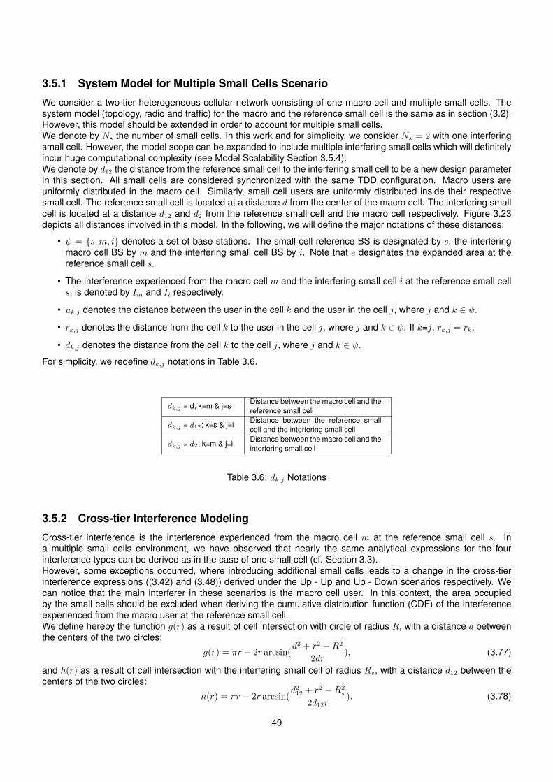
3.5.1 System Model for Multiple Small Cells Scenario
We consider a two-tier heterogeneous cellular network consisting of one macro cell and multiple small cells. Thesystem model (topology, radio and traffic) for the macro and the reference small cell is the same as in section (3.2).However, this model should be extended in order to account for multiple small cells.We denote by Ns the number of small cells. In this work and for simplicity, we consider Ns = 2 with one interferingsmall cell. However, the model scope can be expanded to include multiple interfering small cells which will definitelyincur huge computational complexity (see Model Scalability Section 3.5.4).We denote by d12 the distance from the reference small cell to the interfering small cell to be a new design parameterin this section. All small cells are considered synchronized with the same TDD configuration. Macro users areuniformly distributed in the macro cell. Similarly, small cell users are uniformly distributed inside their respectivesmall cell. The reference small cell is located at a distance d from the center of the macro cell. The interfering smallcell is located at a distance d12 and d2 from the reference small cell and the macro cell respectively. Figure 3.23depicts all distances involved in this model. In the following, we will define the major notations of these distances:
• ψ = {s,m, i} denotes a set of base stations. The small cell reference BS is designated by s, the interferingmacro cell BS by m and the interfering small cell BS by i. Note that e designates the expanded area at thereference small cell s.
• The interference experienced from the macro cell m and the interfering small cell i at the reference small cells, is denoted by Im and Ii respectively.
• uk,j denotes the distance between the user in the cell k and the user in the cell j, where j and k ∈ ψ.
• rk,j denotes the distance from the cell k to the user in the cell j, where j and k ∈ ψ. If k=j, rk,j = rk.
• dk,j denotes the distance from the cell k to the cell j, where j and k ∈ ψ.
For simplicity, we redefine dk,j notations in Table 3.6.
dk,j = d; k=m & j=sDistance between the macro cell and thereference small cell
dk,j = d12; k=s & j=iDistance between the reference smallcell and the interfering small cell
dk,j = d2; k=m & j=iDistance between the macro cell and theinterfering small cell
Table 3.6: dk,j Notations
3.5.2 Cross-tier Interference Modeling
Cross-tier interference is the interference experienced from the macro cell m at the reference small cell s. Ina multiple small cells environment, we have observed that nearly the same analytical expressions for the fourinterference types can be derived as in the case of one small cell (cf. Section 3.3).However, some exceptions occurred, where introducing additional small cells leads to a change in the cross-tierinterference expressions ((3.42) and (3.48)) derived under the Up - Up and Up - Down scenarios respectively. Wecan notice that the main interferer in these scenarios is the macro cell user. In this context, the area occupiedby the small cells should be excluded when deriving the cumulative distribution function (CDF) of the interferenceexperienced from the macro user at the reference small cell.We define hereby the function g(r) as a result of cell intersection with circle of radius R, with a distance d betweenthe centers of the two circles:
g(r) = πr − 2r arcsin(d2 + r2 −R2
2dr), (3.77)
and h(r) as a result of cell intersection with the interfering small cell of radius Rs, with a distance d12 between thecenters of the two circles:
h(r) = πr − 2r arcsin(d212 + r2 −R2
s
2d12r). (3.78)
49
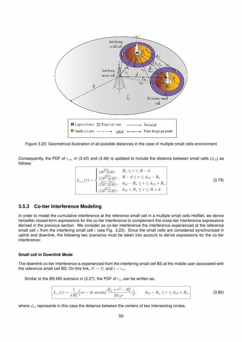
Figure 3.23: Geometrical illustration of all possible distances in the case of multiple small cells environment
Consequently, the PDF of rsm in (3.42) and (3.48) is updated to include the distance between small cells (d12) asfollows:
frsm(r) =
2πr
πR2−2πR2s, Rs ≤ r < R− d
g(r)(πR2−2πR2
s), R− d ≤ r ≤ d12 −Rs
g(r)−h(r)(πR2−2πR2
s), d12 −Rs ≤ r ≤ d12 +Rs
g(r)(πR2−2πR2
s), d12 +Rs ≤ r ≤ R+ d.
(3.79)
3.5.3 Co-tier Interference Modeling
In order to model the cumulative interference at the reference small cell in a multiple small cells HetNet, we derivehereafter closed-form expressions for the co-tier interference to complement the cross-tier interference expressionsderived in the previous section. We consider as co-tier interference the interference experienced at the referencesmall cell s from the interfering small cell i (see Fig. 3.23). Since the small cells are considered synchronized inuplink and downlink, the following two scenarios must be taken into account to derive expressions for the co-tierinterference:
Small cell in Downlink Mode
The downlink co-tier interference is experienced from the interfering small cell BS at the mobile user associated withthe reference small cell BS. On this link, Pt = Ps and l = ris.
Similar to the BS-MS scenario in (3.27), the PDF of ris can be written as:
fris(r) =1
πR2s
(πr − 2r arcsin(
d212 + r2 −R2s
2d12r)), d12 −Rs ≤ r ≤ d12 +Rs, (3.80)
where d12 represents in this case the distance between the centers of two intersecting circles.
50
Small cell in Uplink Mode
The uplink co-tier interference is experienced from the interfering small cell user at the reference small cell BS. Onthis link, Pt = Ps and l = rsi.The PDF of rsi can be obtained as a result of cell intersection with the interfering small cell of radius Rs:
frsi(r) =1
πR2s
(πr − 2r arcsin(
d212 + r2 −R2s
2d12r)), d12 −Rs ≤ r ≤ d12 +Rs. (3.81)
3.5.4 Model Scalability
Although in this section the model is built with two small cells, however its scope can be expanded to include multi-ple interfering small cells f located at distance d1f from the reference small cell respectively. Accordingly, in orderto derive expressions for the interference experienced from different interfering small cells, the PDF of ris (to bedenoted by rfs) in (3.80) is revised by replacing d12 with d1f , same for the PDF of rsi (to be denoted by rsf ) in (3.81).On the other hand, the PDF of the interference experienced from the macro users and thus, the PDF of rsm in (3.79)is carefully revised and can be written as follows:
frsm(r) =
2πrπR2−NsπR2
s, Rs ≤ r < R− d
g(r)(πR2−NsπR2
s), R− d ≤ r ≤ df −Rs
g(r)−∑Nsf=2 hf (r)
(πR2−NsπR2s)
, df −Rs ≤ r ≤ Df +Rsg(r)
(πR2−NsπR2s), Df +Rs ≤ r ≤ R+ d,
(3.82)
where g(r) = πr − 2r arcsin( d2+r2−R2
2dr), Df = max
2≤f≤Nsd1f , df = min
2≤f≤Nsd1f and
hf (r) =
{πr − 2r arcsin(
d21f+r2−R2
s
2d1f r), d1f −Rs ≤ r ≤ d1f +Rs
0, elsewhere.(3.83)
3.5.5 Signal of Interest Modeling
The signal power received by a randomly selected user at the reference small cell on a downlink channel is definedas: S = KL0Psr
−γs where rs is the distance of the user from the small cell BS s. The distribution of S remains the
same as in the case of a single small cell:fS(s) = βs−(
2+γγ ), (3.84)
where β = 2K2γc
γR2s
and Kc = KL0Ps. Note that same logic applies to derive similar expressions on the uplink channel.
3.5.6 Capacity Analysis in Multiple Small Cells Scenario
The average user capacity per unit bandwidth i.e. the spectral efficiency at the reference small cell, in a multiplesmall cells environment is defined as follows:
Cs = E[B ln(1 + S
Itot+σ2 )
B
]= E
[ln(1 +
S
Itot + σ2)], (3.85)
where σ2 is the thermal noise power variance and Itot the cumulative interference defined as: Itot = Im + Ii. Imis the interference experienced from the macro cell and Ii is the interference experienced from the interfering smallcells, at the reference small cell. S and Itot are considered as two independent variables. In the following, we willprovide an approximation to the generic function of the capacity Cs:
The interference, in general, can be written as: I = KL0Ptl−γ = Kcl
−γ where Kc = KL0Pt, l denotes the in-terfering distance, Pt the transmitted power and K the composite fading. Applying the chain rule to the CDF of I,
51
the corresponding PDF can be written as fI(i) = 1iγfl
(( iKc
)−1γ
)( iKc
)−1γ . Accordingly, a closed-form expression for
the MGF of the interference I can be formulated as MI(t) =∫∞0e−tifI(i)di. Note that the same steps apply for the
derivation of the MGF of the signal of interest (MS(t)).Denote by Itot the cumulative interference from the macro cell (Im) and the interfering small cells (Ii), at the ref-erence small cell. Consequently, Itot can be written as: Itot = Im + Ii. Considering Im and Ii as independentvariables, the MGF of the cumulative interference Itot can be calculated as follows: MItot(t) =MIm(t)MIi(t).Based on the MGF expressions derived for S and Itot, the average capacity per unit bandwidth can be calculatedusing the lemma proposed in [112] as follows:
Cs = E[ln(1 + SItot+σ2 )] =
∫∞0
MItot (t)−MS(t)MItot (t)
te−(σ
2)tdt
Cs =∫∞0
MIm (t)MIi(t)−MS(t)MIm (t)MIi
(t)
te−ate−(σ
2+a)tdt.
This expression can be solved efficiently by expressing it in terms of the weights we and abscissas xe of a La-guerre orthogonal polynomial [113] [114], as follows:
Cs =
n∑e=1
we
(MIm(xe/(σ2 + a))MIi(xe/(σ
2 + a))
xee−(axe)/(σ2+a)
− MS(xe/(σ2 + a))MIm(xe/(σ
2 + a))MIi(xe/(σ2 + a))
xee−(axe)/(σ2+a)
). (3.86)
In this work, the a parameter was introduced to resolve the scaling problem in Laguerre polynomial, more specif-ically in the M(t) expression. Adding the a parameter will ensure scalable values of the MGF expression withM(xe/(σ
2 + a)). a is set to 10−4 in the scenarios where the macro cell is in a DL mode and to 10−6 in the scenarioswhere the macro cell is in an UL mode.
Special Case: ψ = {s,m}, i.e. Ns = 1 and Ii = 0: In case of a network consisting of one macro cell andone reference small cell, the latter will be purely affected by the interfering macro cell and therefore Itot = Im = I.Accordingly, the capacity expression can be formulated as follows:
Cs =
n∑e=1
we
(MI(xe/(σ2 + a))
xee−(axe)/(σ2+a)
− MS(xe/(σ2 + a))MI(xe/(σ
2 + a))
xee−(axe)/(σ2+a)
). (3.87)
3.5.7 Uplink Power Control
Uplink power control can also be added to the developed model. Based on the open-loop power control strategystandardized in 3GPP LTE [109], the transmit power of a mobile user is given by:
Pt = min(Pmax, P0rγs ), (3.88)
where rs is the distance of the reference small cell user from its serving BS, P0 is the desired received signal level atthe BS and Pmax denotes the maximum transmit power capability per user. Consequently, the uplink signal powerreceived at the reference BS with power control can be given as S = KL0Ptr
−γs with:
S =
{KL0P0, Pmax > P0r
γs
KL0Pmaxr−γs , Pmax ≤ P0r
γs ,
(3.89)
and the interference caused at a reference BS (or user) from a given interfering small cell (or macro cell), can thenbe derived as I = KL0Ptl
−γ with:
I =
{KL0P0r
γs l−γ , Pmax > P0r
γs
KL0Pmaxl−γ , Pmax ≤ P0r
γs ,
(3.90)
52
where l is the length of the interfering link. The PDF of I can be derived by averaging over rs the PDF of fl(r)|rs .It is important to note that the power control mechanism leads in average to reduction in power consumption whena user in a specific position is able to compensate the overall path loss with P0r
γs < Pmax. In this case, average
reduction in power consumption (PR) can be defined as: PR = E[Pmax − P0rγs ].
Simulation results showing the impact of power control on the system throughput and the network power consump-tion, will be discussed in the next chapter under Section 4.5.2.
3.5.8 Unsynchronized TDD Configuration
Although in this chapter the model is developed based on a synchronized TDD configuration assumption acrosssmall cells, it can be well adapted to consider an unsynchronized TDD configuration by deriving two additionalexpressions for the co-tier interference experienced from the interfering small cell at the reference small cell:
1) In the case where the interfering small cell operates in uplink and the reference small cell operates in downlink,the PDF of the distance from the interfering small cell user to the reference small cell user (uis) can be derivedsimilarly to the PDF of ums in (3.47):
fuis(r) =
∫ r+Rs
r−Rsfuis|rsi(r)frsi(rsi)drsi, 2(Re −Rs) ≤ r ≤ d+ 2Rs, (3.91)
where fuis|rsi(r) =1
πR2s(πr − 2r arcsin( r
2si+r
2−R2s
2rsir)) and frsi(rsi) defined as
follows:
frsi(rsi) =1
πR2s
(πrsi − 2rsi arcsin(
d212 + r2si −R2s
2d12rsi)), (3.92)
2) In the case where the interfering small cell operates in downlink and the reference small cell operates in uplink,the distance from the interfering small cell to the reference small cell is constant and equal to d12.
Simulation results showing the impact of considering an unsynchronized TDD configuration, will be discussed in thenext chapter under Section 4.5.3.
3.5.9 Decoupling Gain Analysis in Multiple Small Cells Scenario
In the previous sections, we have calculated the average user capacity per association policy mainly, in order tocompare the performance of the decoupling strategy with other association strategies. However and in order toprovide more insights about the gain that the decoupling strategy can bring in comparison with the coupled withmacro case, we focus in this section on the analytical evaluation of this gain that is referred to as the decouplinggain. Under this context, we investigate the decoupling gain mainly in multiple small cells scenario where it appearsto be dependent on the distance between the reference small cell and the interfering small cells.
Definition 1. The decoupling gain, denoted as ηd, is defined as the ratio between the throughput achieved whendecoupling is adopted and the throughput achieved without decoupling (in the coupled with macro (CM) case):
ηd =Throughputd(Decoupling) - Throughputd(CM)
Throughputd(CM), (3.93)
where d ∈ {UL,DL}.
To analyze the decoupling gain in a multiple small cells TDD HetNet, it is important to develop a complete modelfor both the CM and the decoupling cases. Moreover, calculating the decoupling gain in one direction (UL or DL)necessitates measuring Ces in that direction for both CM and decoupling cases. Ces is computed by adding theaverage users capacity in the small cell area (Cs) to the average users capacity in the expanded area (Ce). Forsimplicity, we consider in the below calculations Ns = 2 with one interfering small cell.
53
Uplink Decoupling Gain
In the Down - Up and Up - Up scenarios, small cell users along with the users in the expanded area are operatingin uplink. Hence, the latter two scenarios present a considerable part of the overall uplink capacity (Ces), whereasthe Up - Down case considers a negligible part (Ces = Ce ' 0).
A. Down - Up Scenario
a) CM Case: For the Cs calculation, closed-form expressions are derived for:
• Im = KL0Pmd.
• Ii = KL0Pusrsi, where d12 −Rs ≤ rsi ≤ d12 +Rs.
• Ss = KL0Pusrs, where 0 ≤ rs ≤ Rs.
The PDF frsi(r) is given by (3.81), an expression derived in the case of two small cells:
frsi(r) =1
πR2s
(πr − 2r arcsin(
d212 + r2 −R2s
2d12r)), d12 −Rs ≤ r ≤ d12 +Rs. (3.94)
In this case, Ce = 0.b) Decoupling Case: For the Cs calculation, closed-form expressions are derived for:
• Im = KL0Pmd.
• Ii = KL0Pusrsi, where d12 −Re ≤ rsi ≤ d12 +Re.
• Ss = KL0Pusrs, where 0 ≤ rs ≤ Rs.
The PDF frsi(r) is given by replacing Rs with Re in (3.94):
frsi(r) =1
πR2e
(πr − 2r arcsin(
d212 + r2 −R2e
2d12r)), d12 −Re ≤ r ≤ d12 +Re. (3.95)
The same interference expressions will be derived for the calculation of Ce. However, Se is defined as: Se =KL0Pusre, where Rs ≤ re ≤ Re.
B. Up - Up Scenario
a) CM Case: For the Cs calculation, closed-form expressions are derived for:
• Im = KL0Pumrsm, where Rs ≤ rsm ≤ R+ d.
• Ii = KL0Pusrsi, where d12 −Rs ≤ rsi ≤ d12 +Rs.
• Ss = KL0Pusrs, where 0 ≤ rs ≤ Rs.
The PDF of rsm is derived as follows:
frsm(r) =
2πr
(πR2−2πR2s), Rs ≤ r < R− d
g(r)(πR2−2πR2
s), R− d ≤ r ≤ d12 −Rs
g(r)−h(r)(πR2−2πR2
s), d12 −Rs ≤ r ≤ d12 +Rs
g(r)(πR2−2πR2
s), d12 +Rs ≤ r ≤ R+ d,
(3.96)
where g(r) = πr − 2r arcsin( d2+r2−R2
2dr) and h(r) = πr − 2r arcsin( d
212+r
2−R2s
2d12r).
The PDF of rsi is given by (3.94).In this case, Ce ' 0.
b) Decoupling Case: For the Cs calculation, closed-form expressions are derived for:
54
• Im = KL0Pumrsm, where Re ≤ rsm ≤ R+ d.
• Ii = KL0Pusrsi, where d12 −Re ≤ rsi ≤ d12 +Re.
• Ss = KL0Pusrs, where 0 ≤ rs ≤ Rs.
The PDF frsm(r) is given by replacing Rs with Re in (3.96):
frsm(r) =
2πr
(πR2−2πR2e), Re ≤ r < R− d
g(r)(πR2−2πR2
e), R− d ≤ r ≤ d12 −Re
g(r)−i(r)(πR2−2πR2
e), d12 −Re ≤ r ≤ d12 +Re
g(r)(πR2−2πR2
e), d12 +Re ≤ r ≤ R+ d,
(3.97)
where g(r) = πr − 2r arcsin( d2+r2−R2
2dr) and i(r) computed as a result of cell intersection with the interfering small
cell of radius Re, with a distance d12 between the centers of the two circles:
i(r) = πr − 2r arcsin(d212 + r2 −R2
e
2d12r). (3.98)
The PDF of rsi is given by (3.95).The same interference expressions will be derived for the calculation of Ce. However, Se is defined as: Se =KL0Pusre.
Downlink Decoupling Gain
In the Up - Down and Down - Down scenarios, small cell users along with the users in the expanded area areoperating in downlink. Hence, the latter two scenarios present a considerable part of the overall downlink capacity(Ces), whereas the Down - Up case considers a negligible part (Ces = Ce ' 0).
A. Up - Down Scenario
a) CM Case: For the Cs calculation, closed-form expressions are derived for:
• Im = KL0Pumums, where 0 ≤ ums ≤ R+ d+Rs.
• Ii = KL0Psris, where d12 −Rs ≤ ris ≤ d12 +Rs.
• Ss = KL0Psrs, where 0 ≤ rs ≤ Rs.
ums represents the distance from the macro cell user to the small cell user that is located inside the area boundedby Rs. The PDF of ums is derived by averaging over the PDF of rsm (frsm(rsm)):
fums(r) =
∫ r+Rs
r−Rsfums|rsm(r)frsm(rsm)drsm, 0 ≤ r ≤ R+ d+Rs, (3.99)
where rsm is the distance of the reference small cell BS from the macro cell user and fums|rsm(r) denotes the PDFof ums conditioned on rsm.In this case, the expanded areas of both small cells are part of the macro user region and thus, frsm will be derivedusing Rs as the main parameter to determine the macro user area boundaries as in (3.96). Since Cs represents theaverage capacity of the reference small cell users located inside the area bounded by Rs, the integral of fums|rsm(r)will range from r − Rs to r + Rs. The PDF fris(r) is given by (3.80), an expression derived in the case of two smallcells:
fris(r) =1
πR2s
(πr − 2r arcsin(
d212 + r2 −R2s
2d12r)), d12 −Rs ≤ r ≤ d12 +Rs. (3.100)
In the CM case under the Up - Down scenario, Ce = 0 and thus, Ces = Cs.b) Decoupling Case: For the Cs calculation, closed-form expressions are derived for:
• Im = KL0Pumums, where Re −Rs ≤ ums ≤ R+ d+Rs.
55
• Ii = KL0Psris, where d12 −Rs ≤ ris ≤ d12 +Rs.
• Ss = KL0Psrs, where 0 ≤ rs ≤ Rs.
ums represents the distance from the macro cell user to the small cell user that is located inside the area boundedby Rs. The PDF of ums is derived by averaging over the PDF of rsm (frsm(rsm)):
fums(r) =
∫ r+Rs
r−Rsfums|rsm(r)frsm(rsm)drsm, Re −Rs ≤ r ≤ R+ d+Rs. (3.101)
Contrary to the CM case, the expanded areas of both small cells are out of the macro user region and thus, frsm willbe derived using Re as the main parameter to determine the macro user area boundaries:
frsm(r) =
2πr
(πR2−2πR2e), Re ≤ r < R− d
g(r)(πR2−2πR2
e), R− d ≤ r ≤ d12 −Re
g(r)−i(r)(πR2−2πR2
e), d12 −Re ≤ r ≤ d12 +Re
g(r)(πR2−2πR2
e), d12 +Re ≤ r ≤ R+ d,
(3.102)
where g(r) = πr − 2r arcsin( d2+r2−R2
2dr) and i(r) = πr − 2r arcsin( d
212+r
2−R2e
2d12r).
Consequently, ums will range from Re − Rs to R + d + Rs. Similar to the CM case and since Cs represents theaverage capacity of the reference small cell users located inside the area bounded by Rs, the integral of fums|rsm(r)will range from r −Rs to r +Rs.Note that ris(r) follows the same statistical distribution as in the CM case. Whether the user located in the expandedarea, is in decoupling or CM state, ris(r) will be reflecting the interference experienced from the interfering smallcell independently of the small cell user access policy.In this case, Ce = 0 and thus, Ces = Cs.
B. Down - Down Scenario
Under this scenario, same expressions are derived for both CM and decoupling cases. Theoretically, it meansthere is no downlink decoupling gain (ηDL = 0).For the Cs calculation, closed-form expressions are derived for:
• Im = KL0Pmrms, where d−Rs ≤ rms ≤ d+Rs.
• Ii = KL0Psris, where d12 −Rs ≤ ris ≤ d12 +Rs.
• Ss = KL0Psrs, where 0 ≤ rs ≤ Rs.
The PDF of rms can be obtained as a result of the cell intersection with the circle of radius Rs:
frms(r) =1
πR2s
(πr − 2r arcsin(
d2 + r2 −R2s
2dr)), d−Rs ≤ r ≤ d+Rs. (3.103)
The PDF of ris is given by (3.100).As for the Ce calculation, closed-form expressions are derived for:
• Im = KL0Pmrme, where d−Re ≤ rme ≤ d+Re.
• Ii = KL0Psrie, where d12 −Re ≤ rie ≤ d12 +Re.
• Se = KL0Psre, where Rs ≤ re ≤ Re.
The PDF of rme can be defined similarly as in (3.60). As for the distribution of rie, it is given by replacing d with d12in (3.60):
56
frie(r) =
i(r)
(πR2e−πR2
s), d12 −Re ≤ r ≤ d12 −Rs
i(r)−h(r)(πR2
e−πR2s), d12 −Rs ≤ r ≤ d12 +Rs
i(r)(πR2
e−πR2s), d12 +Rs ≤ r ≤ d12 +Re,
(3.104)
where i(r) = πr − 2r arcsin( d212+r
2−R2e
2d12r) and h(r) = πr − 2r arcsin(
d212+r2−R2
s
2d12r).
3.6 Conclusion
In this chapter, we have developed a statistical and analytical model for a HetNet based system where decou-pling and dynamic TDD are jointly deployed. The proposed model offers a simple analysis tool to assess a givenTDD/Decoupling-based HetNet deployment. The analytical formulas provide relevant insights about network perfor-mance without the need for time consuming Monte-Carlo Simulations. This tool is also useful for network designerswho can use it to determine the range of deployment parameters given a target QoS.In our analysis, we have considered a network consisting of one macro cell along with one small cell. Our mainfocus will be evaluating users’ performance inside the small cell. This small cell is referred to as a reference smallcell.Firstly, the case of one small cell has been considered. Incorporating the dynamic TDD technique into the HetNetbased system has imposed the modeling of four kinds of cross-tier interference in order to cover all UL/DL TDDpossible combinations between the macro cell from a side and the small cell from the other side. Moreover, deploy-ing the decoupling policy on top of the TDD HetNet system has necessitated the modeling of various associationpolicies in order to highlight the benefits that the decoupling policy can bring to that system in comparison with theother policies.Secondly, multiple instances of interfering small cells have been deployed at specific distances from the referencesmall cell in order to be aligned as much as possible with real case scenarios. We have considered this specificnetwork model, as simple as it shows in regards to BS distribution, to focus on the main thesis objective which isthe modeling of TDD and decoupling in a scenario that is close to real cases, and at the same time to avoid addingfurther complexity to the model itself. Instead, including any other BS distribution (stochastic for example) will bringsignificant additional complexity to our HetNet analysis. In this case, our work will be further away from reaching itsobjectives.In this chapter, a geometric approach has been adopted to derive closed-form expressions for the interfering dis-tances along with the location of the reference small cell user. This geometric approach was based on differentmethods, e.g. cells intersection method, randomly selected nodes in concentric circles method, etc. Based onthe distances distribution, we have calculated the PDF and MGF of the interference and the signal of interest. Inmultiple small cells environment, a new type of interference to which we refer to as the co-tier interference has beenmodeled in addition to the cross-tier interference. Relying on the MGF results of both the interference and the signalof interest, we have derived closed-form expression for the spectral efficiency or what we refer to as capacity perunit bandwidth. Also, additional expressions have been derived for other performance metrics. e.g. the decouplinggain, power control and average reduction in power consumption. Moreover, the statistical model has been adaptedto consider an unsynchronized TDD configuration across small cells, in addition to the initial synchronized TDDconfiguration.
57

Chapter 4
Performance Evaluation of TDD andDecoupling in 5G HetNets
4.1 Introduction
We evaluate under this chapter the system performance metrics, for which we have derived closed form expressionsin Chapter 3. We define the system parameters and discuss the Monte-Carlo simulation results that are provided tovalidate the accuracy of the analytical model including 95% confidence intervals of disparity measures. Confidenceintervals are derived for a sample mean, using the sample data values themselves. In this chapter, we denote by(Th.) the theoretical results and by (M.C.) the Monte-Carlo simulation results.
4.2 System Parameters
In this chapter, we consider analyzing the average capacity (Ces) of the reference small cell for each of the belowlisted scenarios. Ces is computed by adding the average users capacity in the small cell area (Cs) to the averageusers capacity in the expanded area (Ce). Uniformly distributed users are considered in both macro and small cells.The default system parameters are listed in Table 4.1. According to 3GPP standards, macro cell radius can be setfrom few kilometers up to 35 Km. In this model, we consider a macro cell radius R = 1 Km with a maximum BStransmission power Pm = 43 dBm (20 W) according to the 3GPP specifications in [118]. In this case, the powerreceived at the macro cell edge will be around -85 dBm, which is considered as the minimum desired received signallevel at the mobile user. The power received at the cell edge was calculated based on the path-loss expression in(3.1) or (3.2), leading to a path-loss constant L0 = 1.58 ∗ 10−4. As for the small cell coverage, the radius can betypically set between 10 and 250 m. In this model, we consider a small cell radius Rs = 200 m with a maximumtransmission power Ps = 24 dBm (0.25 W) according to the 3GPP specifications in [119]. Similarly to the macro cellcase, the power received at the small cell edge will be around -83 dBm. The maximum UE transmission power isset to 23 dBm (0.22 W) according to [118].Yet, in order to apply a sort of power control between macro cell users from one side and small cell users fromthe other side, we allow a slight difference between UE maximum transmission power in macro cell Pum = 23.4dBm (0.22 W) and Pus = 23 dBm (0.2 W) in small cells. However, in Section 4.5.2 a dynamic uplink power controlmechanism is considered instead. The latter is based on the open-loop power control strategy with a desiredreceived signal level at the BS, P0 = 10−7 W (-40 dBm) [109].
4.2.1 TDD Frame Type
In this Chapter, we consider frame structures where all uplink/downlink combinations between the macro and smallcells are taken into account, as shown in Fig. 4.1. In the sections that follow, both UL and DL throughputs will beevaluated and averaged over the period of the TDD frame defined in this figure.It is important to note that, relying on the model developed in Chapter 3 and that encloses all possible inter-linkinterferences, any other TDD configuration with different length can be easily adopted and investigated.
59
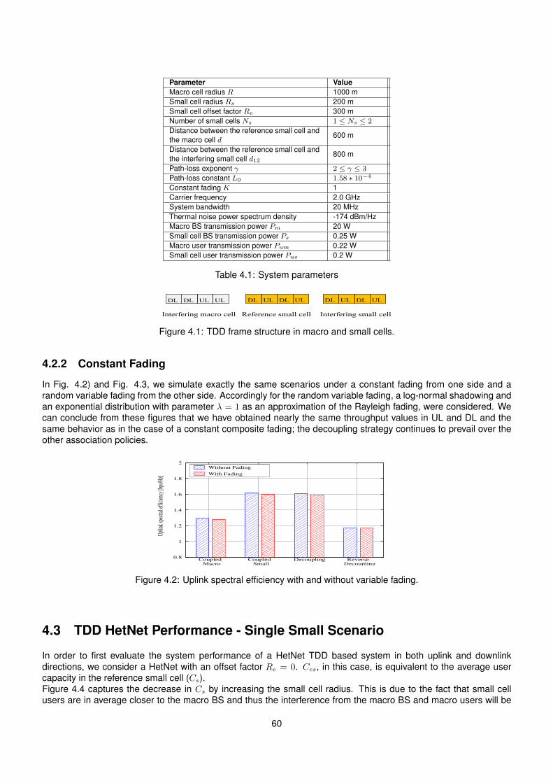
Parameter ValueMacro cell radius R 1000 mSmall cell radius Rs 200 mSmall cell offset factor Re 300 mNumber of small cells Ns 1 ≤ Ns ≤ 2
Distance between the reference small cell andthe macro cell d
600 m
Distance between the reference small cell andthe interfering small cell d12
800 m
Path-loss exponent γ 2 ≤ γ ≤ 3
Path-loss constant L0 1.58 ∗ 10−4
Constant fading K 1Carrier frequency 2.0 GHzSystem bandwidth 20 MHzThermal noise power spectrum density -174 dBm/HzMacro BS transmission power Pm 20 WSmall cell BS transmission power Ps 0.25 WMacro user transmission power Pum 0.22 WSmall cell user transmission power Pus 0.2 W
Table 4.1: System parameters
ULDLDL
Interfering macro cell
UL
Reference small cell Interfering small cell
DLULDL UL DLULDL UL
Figure 4.1: TDD frame structure in macro and small cells.
4.2.2 Constant Fading
In Fig. 4.2) and Fig. 4.3, we simulate exactly the same scenarios under a constant fading from one side and arandom variable fading from the other side. Accordingly for the random variable fading, a log-normal shadowing andan exponential distribution with parameter λ = 1 as an approximation of the Rayleigh fading, were considered. Wecan conclude from these figures that we have obtained nearly the same throughput values in UL and DL and thesame behavior as in the case of a constant composite fading; the decoupling strategy continues to prevail over theother association policies.
0.8
1
1.2
1.4
1.6
1.8
2
Coupled Macro
Coupled Small
Decoupling Reverse Decoupling
Upl
ink
spec
tral e
ffici
ency
[bps
/Hz]
Without Fading
With Fading
Figure 4.2: Uplink spectral efficiency with and without variable fading.
4.3 TDD HetNet Performance - Single Small Scenario
In order to first evaluate the system performance of a HetNet TDD based system in both uplink and downlinkdirections, we consider a HetNet with an offset factor Re = 0. Ces, in this case, is equivalent to the average usercapacity in the reference small cell (Cs).Figure 4.4 captures the decrease in Cs by increasing the small cell radius. This is due to the fact that small cellusers are in average closer to the macro BS and thus the interference from the macro BS and macro users will be
60
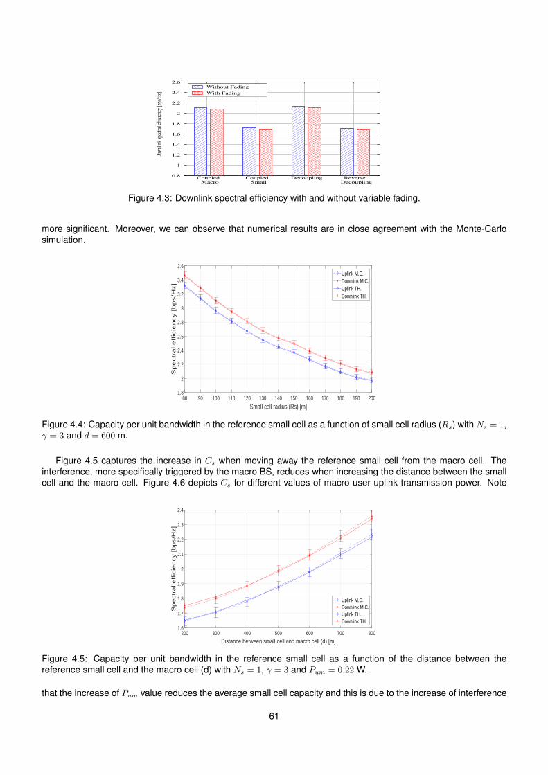
0.8
1
1.2
1.4
1.6
1.8
2
2.2
2.4
2.6
Coupled Macro
Coupled Small
Decoupling Reverse Decoupling
Dow
nlin
k sp
ectra
l effi
cien
cy [b
ps/H
z]
Without Fading
With Fading
Figure 4.3: Downlink spectral efficiency with and without variable fading.
more significant. Moreover, we can observe that numerical results are in close agreement with the Monte-Carlosimulation.
Small cell radius (Rs) [m]80 90 100 110 120 130 140 150 160 170 180 190 200
Sp
ectr
al e
ffic
ien
cy [
bp
s/H
z]
1.8
2
2.2
2.4
2.6
2.8
3
3.2
3.4
3.6Uplink M.C.Downlink M.C.Uplink TH.Downlink TH.
Figure 4.4: Capacity per unit bandwidth in the reference small cell as a function of small cell radius (Rs) with Ns = 1,γ = 3 and d = 600 m.
Figure 4.5 captures the increase in Cs when moving away the reference small cell from the macro cell. Theinterference, more specifically triggered by the macro BS, reduces when increasing the distance between the smallcell and the macro cell. Figure 4.6 depicts Cs for different values of macro user uplink transmission power. Note
Distance between small cell and macro cell (d) [m]200 300 400 500 600 700 800
Sp
ectr
al e
ffic
ien
cy [
bp
s/H
z]
1.6
1.7
1.8
1.9
2
2.1
2.2
2.3
2.4
Uplink M.C.Downlink M.C.Uplink TH.Downlink TH.
Figure 4.5: Capacity per unit bandwidth in the reference small cell as a function of the distance between thereference small cell and the macro cell (d) with Ns = 1, γ = 3 and Pum = 0.22 W.
that the increase of Pum value reduces the average small cell capacity and this is due to the increase of interference
61
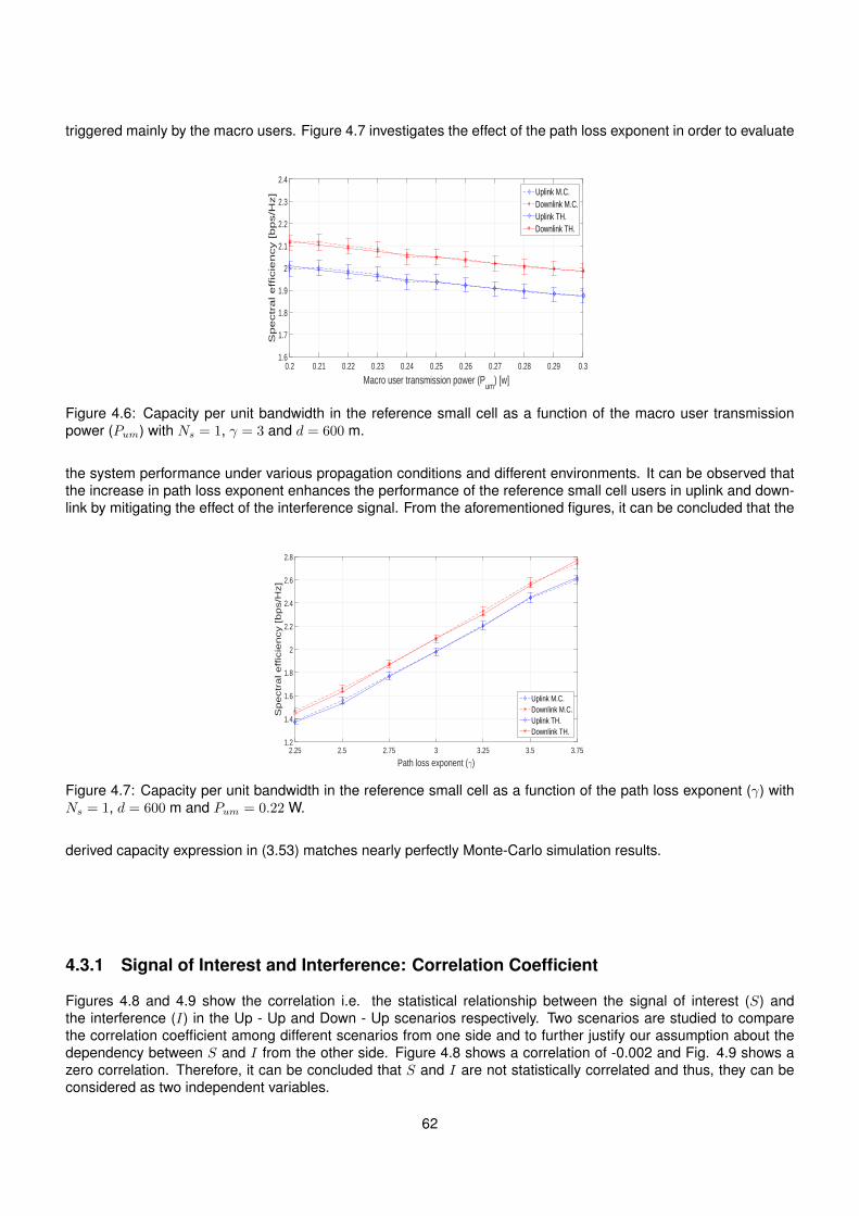
triggered mainly by the macro users. Figure 4.7 investigates the effect of the path loss exponent in order to evaluate
Macro user transmission power (Pum
) [w]0.2 0.21 0.22 0.23 0.24 0.25 0.26 0.27 0.28 0.29 0.3
Sp
ectr
al e
ffic
ien
cy [
bp
s/H
z]
1.6
1.7
1.8
1.9
2
2.1
2.2
2.3
2.4Uplink M.C.Downlink M.C.Uplink TH.Downlink TH.
Figure 4.6: Capacity per unit bandwidth in the reference small cell as a function of the macro user transmissionpower (Pum) with Ns = 1, γ = 3 and d = 600 m.
the system performance under various propagation conditions and different environments. It can be observed thatthe increase in path loss exponent enhances the performance of the reference small cell users in uplink and down-link by mitigating the effect of the interference signal. From the aforementioned figures, it can be concluded that the
Path loss exponent (γ)2.25 2.5 2.75 3 3.25 3.5 3.75
Sp
ectr
al e
ffic
ien
cy [
bp
s/H
z]
1.2
1.4
1.6
1.8
2
2.2
2.4
2.6
2.8
Uplink M.C.Downlink M.C.Uplink TH.Downlink TH.
Figure 4.7: Capacity per unit bandwidth in the reference small cell as a function of the path loss exponent (γ) withNs = 1, d = 600 m and Pum = 0.22 W.
derived capacity expression in (3.53) matches nearly perfectly Monte-Carlo simulation results.
4.3.1 Signal of Interest and Interference: Correlation Coefficient
Figures 4.8 and 4.9 show the correlation i.e. the statistical relationship between the signal of interest (S) andthe interference (I) in the Up - Up and Down - Up scenarios respectively. Two scenarios are studied to comparethe correlation coefficient among different scenarios from one side and to further justify our assumption about thedependency between S and I from the other side. Figure 4.8 shows a correlation of -0.002 and Fig. 4.9 shows azero correlation. Therefore, it can be concluded that S and I are not statistically correlated and thus, they can beconsidered as two independent variables.
62
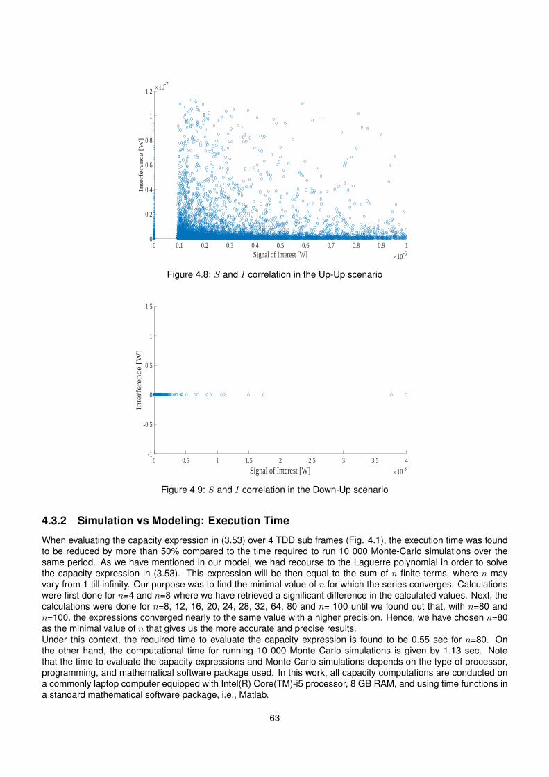
Signal of Interest [W]×10-6
0 0.1 0.2 0.3 0.4 0.5 0.6 0.7 0.8 0.9 1
Inte
rfere
nce [
W]
×10-7
0
0.2
0.4
0.6
0.8
1
1.2
Figure 4.8: S and I correlation in the Up-Up scenario
Signal of Interest [W] ×10-30 0.5 1 1.5 2 2.5 3 3.5 4
Inte
rfere
nce [
W]
-1
-0.5
0
0.5
1
1.5
Figure 4.9: S and I correlation in the Down-Up scenario
4.3.2 Simulation vs Modeling: Execution Time
When evaluating the capacity expression in (3.53) over 4 TDD sub frames (Fig. 4.1), the execution time was foundto be reduced by more than 50% compared to the time required to run 10 000 Monte-Carlo simulations over thesame period. As we have mentioned in our model, we had recourse to the Laguerre polynomial in order to solvethe capacity expression in (3.53). This expression will be then equal to the sum of n finite terms, where n mayvary from 1 till infinity. Our purpose was to find the minimal value of n for which the series converges. Calculationswere first done for n=4 and n=8 where we have retrieved a significant difference in the calculated values. Next, thecalculations were done for n=8, 12, 16, 20, 24, 28, 32, 64, 80 and n= 100 until we found out that, with n=80 andn=100, the expressions converged nearly to the same value with a higher precision. Hence, we have chosen n=80as the minimal value of n that gives us the more accurate and precise results.Under this context, the required time to evaluate the capacity expression is found to be 0.55 sec for n=80. Onthe other hand, the computational time for running 10 000 Monte Carlo simulations is given by 1.13 sec. Notethat the time to evaluate the capacity expressions and Monte-Carlo simulations depends on the type of processor,programming, and mathematical software package used. In this work, all capacity computations are conducted ona commonly laptop computer equipped with Intel(R) Core(TM)-i5 processor, 8 GB RAM, and using time functions ina standard mathematical software package, i.e., Matlab.
63
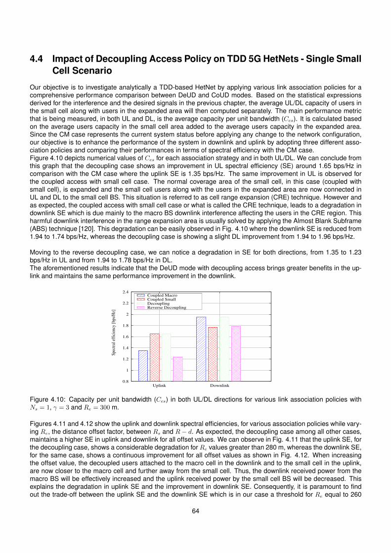
4.4 Impact of Decoupling Access Policy on TDD 5G HetNets - Single SmallCell Scenario
Our objective is to investigate analytically a TDD-based HetNet by applying various link association policies for acomprehensive performance comparison between DeUD and CoUD modes. Based on the statistical expressionsderived for the interference and the desired signals in the previous chapter, the average UL/DL capacity of users inthe small cell along with users in the expanded area will then computed separately. The main performance metricthat is being measured, in both UL and DL, is the average capacity per unit bandwidth (Ces). It is calculated basedon the average users capacity in the small cell area added to the average users capacity in the expanded area.Since the CM case represents the current system status before applying any change to the network configuration,our objective is to enhance the performance of the system in downlink and uplink by adopting three different asso-ciation policies and comparing their performances in terms of spectral efficiency with the CM case.Figure 4.10 depicts numerical values of Ces for each association strategy and in both UL/DL. We can conclude fromthis graph that the decoupling case shows an improvement in UL spectral efficiency (SE) around 1.65 bps/Hz incomparison with the CM case where the uplink SE is 1.35 bps/Hz. The same improvement in UL is observed forthe coupled access with small cell case. The normal coverage area of the small cell, in this case (coupled withsmall cell), is expanded and the small cell users along with the users in the expanded area are now connected inUL and DL to the small cell BS. This situation is referred to as cell range expansion (CRE) technique. However andas expected, the coupled access with small cell case or what is called the CRE technique, leads to a degradation indownlink SE which is due mainly to the macro BS downlink interference affecting the users in the CRE region. Thisharmful downlink interference in the range expansion area is usually solved by applying the Almost Blank Subframe(ABS) technique [120]. This degradation can be easily observed in Fig. 4.10 where the downlink SE is reduced from1.94 to 1.74 bps/Hz, whereas the decoupling case is showing a slight DL improvement from 1.94 to 1.96 bps/Hz.
Moving to the reverse decoupling case, we can notice a degradation in SE for both directions, from 1.35 to 1.23bps/Hz in UL and from 1.94 to 1.78 bps/Hz in DL.The aforementioned results indicate that the DeUD mode with decoupling access brings greater benefits in the up-link and maintains the same performance improvement in the downlink.
0.8
1
1.2
1.4
1.6
1.8
2
2.2
2.4
Uplink Downlink
Spe
ctra
l eff
icie
ncy
[bps
/Hz]
Coupled MacroCoupled SmallDecouplingReverse Decoupling
Figure 4.10: Capacity per unit bandwidth (Ces) in both UL/DL directions for various link association policies withNs = 1, γ = 3 and Re = 300 m.
Figures 4.11 and 4.12 show the uplink and downlink spectral efficiencies, for various association policies while vary-ing Re, the distance offset factor, between Rs and R − d. As expected, the decoupling case among all other cases,maintains a higher SE in uplink and downlink for all offset values. We can observe in Fig. 4.11 that the uplink SE, forthe decoupling case, shows a considerable degradation for Re values greater than 280 m, whereas the downlink SE,for the same case, shows a continuous improvement for all offset values as shown in Fig. 4.12. When increasingthe offset value, the decoupled users attached to the macro cell in the downlink and to the small cell in the uplink,are now closer to the macro cell and further away from the small cell. Thus, the downlink received power from themacro BS will be effectively increased and the uplink received power by the small cell BS will be decreased. Thisexplains the degradation in uplink SE and the improvement in downlink SE. Consequently, it is paramount to findout the trade-off between the uplink SE and the downlink SE which is in our case a threshold for Re equal to 260
64
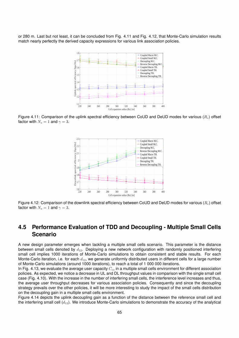
or 280 m. Last but not least, it can be concluded from Fig. 4.11 and Fig. 4.12, that Monte-Carlo simulation resultsmatch nearly perfectly the derived capacity expressions for various link association policies.
Cell expansion radius (Re) [m]220 240 260 280 300 320 340 360 380 400
Up
lin
k s
pec
tral
eff
icie
ncy
[b
ps/
Hz]
1.1
1.2
1.3
1.4
1.5
1.6
1.7
1.8Coupled Macro M.C.Coupled Small M.C.Decoupling M.C.Reverse Decoupling M.C.Coupled Macro TH.Coupled Small TH.Decoupling TH.Reverse Decoupling TH.
Figure 4.11: Comparison of the uplink spectral efficiency between CoUD and DeUD modes for various (Re) offsetfactor with Ns = 1 and γ = 3.
Cell expansion radius (Re) [m]220 240 260 280 300 320 340 360 380 400
Do
wn
lin
k s
pectr
al
eff
icie
ncy
[b
ps/
Hz]
1.6
1.7
1.8
1.9
2
2.1
2.2
2.3Coupled Macro M.C.Coupled Small M.C.Decoupling M.C.Reverse Decoupling M.C.Coupled Macro TH.Coupled Small TH.Decoupling TH.Reverse Decoupling TH.
Figure 4.12: Comparison of the downlink spectral efficiency between CoUD and DeUD modes for various (Re) offsetfactor with Ns = 1 and γ = 3.
4.5 Performance Evaluation of TDD and Decoupling - Multiple Small CellsScenario
A new design parameter emerges when tackling a multiple small cells scenario. This parameter is the distancebetween small cells denoted by d12. Deploying a new network configuration with randomly positioned interferingsmall cell implies 1000 iterations of Monte-Carlo simulations to obtain consistent and stable results. For eachMonte-Carlo iteration, i.e. for each d12, we generate uniformly distributed users in different cells for a large numberof Monte-Carlo simulations (around 1000 iterations), to reach a total of 1 000 000 iterations.In Fig. 4.13, we evaluate the average user capacity Ces in a multiple small cells environment for different associationpolicies. As expected, we notice a decrease in UL and DL throughput values in comparison with the single small cellcase (Fig. 4.10). With the increase in the number of interfering small cells, the interference level increases and thus,the average user throughput decreases for various association policies. Consequently and since the decouplingstrategy prevails over the other policies, it will be more interesting to study the impact of the small cells distributionon the decoupling gain in a multiple small cells environment.Figure 4.14 depicts the uplink decoupling gain as a function of the distance between the reference small cell andthe interfering small cell (d12). We introduce Monte-Carlo simulations to demonstrate the accuracy of the analytical
65
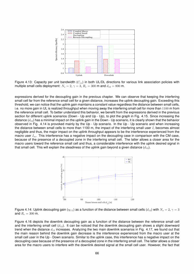
0.8
1
1.2
1.4
1.6
1.8
2
2.2
2.4
2.6
Uplink Downlink
Spe
ctra
l eff
icie
ncy
[bps
/Hz]
Coupled MacroCoupled SmallDecouplingReverse Decoupling
Figure 4.13: Capacity per unit bandwidth (Ces) in both UL/DL directions for various link association policies withmultiple small cells deployment: Ns = 2, γ = 3, Re = 300 m and d12 = 800 m.
expressions derived for the decoupling gain in the previous chapter. We can observe that keeping the interferingsmall cell far from the reference small cell for a given distance, increases the uplink decoupling gain. Exceeding thisthreshold, we can notice that the uplink gain maintains a constant value regardless the distance between small cells,i.e. no more gain in UL is realized throughput when moving away the interfering small cell for more than 1100 m fromthe reference small cell. To better understand this behavior, we benefit from the expressions derived in the previoussection for different uplink scenarios (Down - Up and Up - Up), to plot the graph in Fig. 4.15. Since increasing thedistance (d12) has a minimal impact on the uplink gain in the Down - Up scenario, it is clearly shown that the behaviorobserved in Fig. 4.14 is provoked mainly by the Up - Up scenario. In the Up - Up scenario and when increasingthe distance between small cells to more than 1100 m, the impact of the interfering small user Ii becomes almostnegligible and thus, the major impact on the uplink throughput appears to be the interference experienced from themacro user Im. This interference has a negative impact on the decoupling case in comparison with the CM case,because of the presence of a decoupled zone in the interfering small cell. The latter allows a closer area for themacro users toward the reference small cell and thus, a considerable interference with the uplink desired signal inthat small cell. This will explain the steadiness of the uplink gain beyond a given distance (d12).
Distance between small cells (d12
) [m]800 900 1000 1100 1200
Upli
nk d
ecoupli
ng g
ain
[%
]
25
30
35
40M.C.TH.
Figure 4.14: Uplink decoupling gain (ηUL) as a function of the distance between small cells (d12) with Ns = 2, γ = 3and Re = 300 m.
Figure 4.16 depicts the downlink decoupling gain as a function of the distance between the reference small celland the interfering small cell (d12). It can be noticed that the downlink decoupling gain shows a slight downwardtrend when the distance d12 increases. Analyzing the two main downlink scenarios in Fig. 4.17, we found out thatthe main reason behind the downlink gain decrease is the interference experienced from the macro user at thesmall cell user in the Up - Down scenario. Similar to the uplink case, this interference has a negative impact on thedecoupling case because of the presence of a decoupled zone in the interfering small cell. The latter allows a closerarea for the macro users to interfere with the downlink desired signal at the small cell user. However, the fact that
66
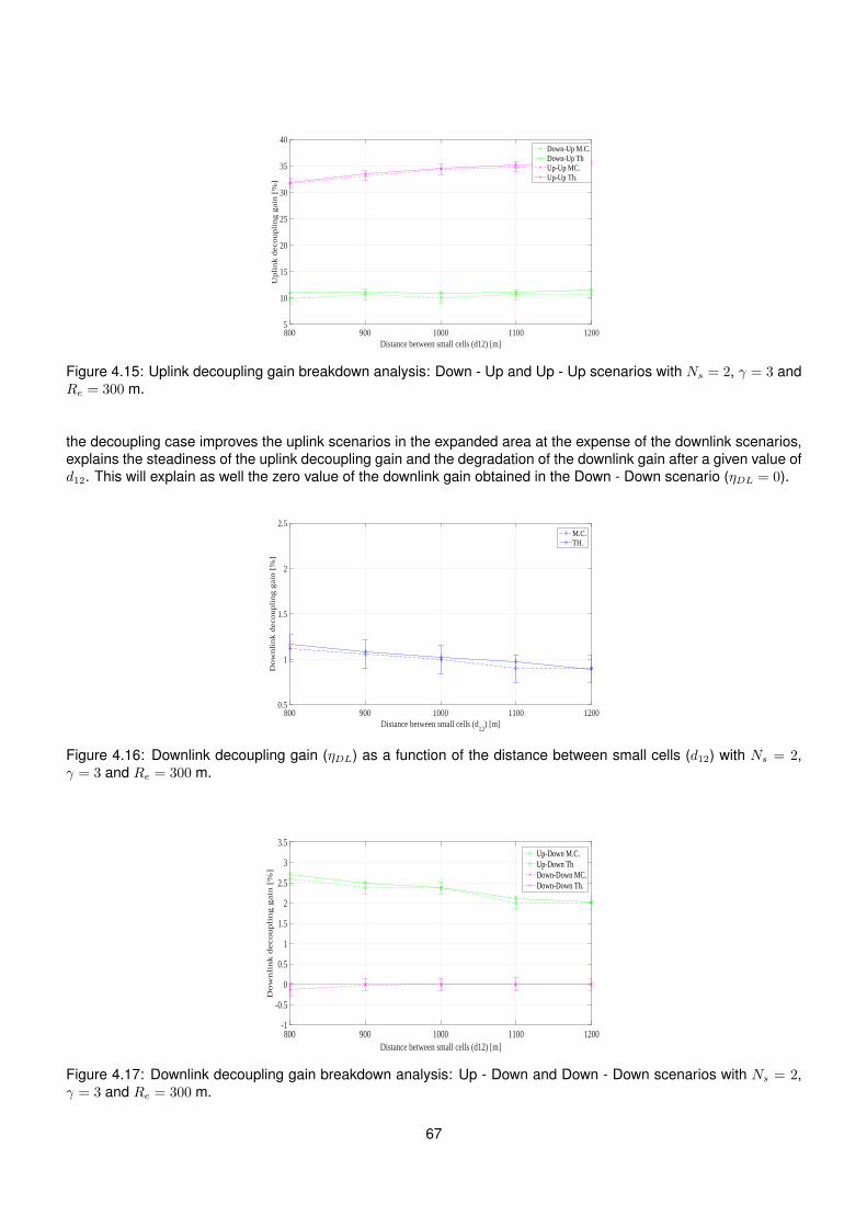
Distance between small cells (d12) [m]800 900 1000 1100 1200
Up
lin
k d
eco
up
lin
g g
ain
[%
]
5
10
15
20
25
30
35
40Down-Up M.C.Down-Up ThUp-Up MC.Up-Up Th.
Figure 4.15: Uplink decoupling gain breakdown analysis: Down - Up and Up - Up scenarios with Ns = 2, γ = 3 andRe = 300 m.
the decoupling case improves the uplink scenarios in the expanded area at the expense of the downlink scenarios,explains the steadiness of the uplink decoupling gain and the degradation of the downlink gain after a given value ofd12. This will explain as well the zero value of the downlink gain obtained in the Down - Down scenario (ηDL = 0).
Distance between small cells (d12
) [m]800 900 1000 1100 1200
Do
wn
lin
k d
eco
up
lin
g g
ain
[%
]
0.5
1
1.5
2
2.5M.C.TH.
Figure 4.16: Downlink decoupling gain (ηDL) as a function of the distance between small cells (d12) with Ns = 2,γ = 3 and Re = 300 m.
Distance between small cells (d12) [m]800 900 1000 1100 1200
Do
wn
lin
k d
eco
up
lin
g g
ain
[%
]
-1
-0.5
0
0.5
1
1.5
2
2.5
3
3.5Up-Down M.C.Up-Down ThDown-Down MC.Down-Down Th.
Figure 4.17: Downlink decoupling gain breakdown analysis: Up - Down and Down - Down scenarios with Ns = 2,γ = 3 and Re = 300 m.
67
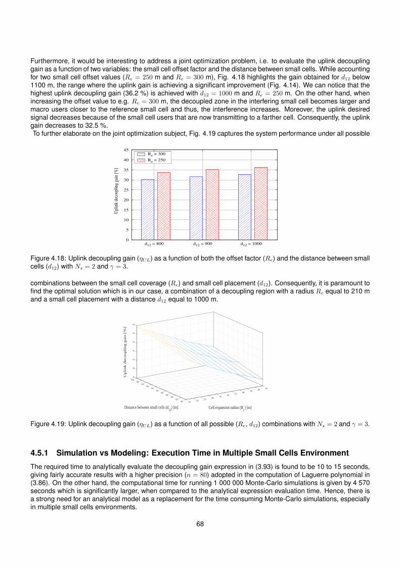
Furthermore, it would be interesting to address a joint optimization problem, i.e. to evaluate the uplink decouplinggain as a function of two variables: the small cell offset factor and the distance between small cells. While accountingfor two small cell offset values (Re = 250 m and Re = 300 m), Fig. 4.18 highlights the gain obtained for d12 below1100 m, the range where the uplink gain is achieving a significant improvement (Fig. 4.14). We can notice that thehighest uplink decoupling gain (36.2 %) is achieved with d12 = 1000 m and Re = 250 m. On the other hand, whenincreasing the offset value to e.g. Re = 300 m, the decoupled zone in the interfering small cell becomes larger andmacro users closer to the reference small cell and thus, the interference increases. Moreover, the uplink desiredsignal decreases because of the small cell users that are now transmitting to a farther cell. Consequently, the uplinkgain decreases to 32.5 %.To further elaborate on the joint optimization subject, Fig. 4.19 captures the system performance under all possible
0
5
10
15
20
25
30
35
40
45
d12 = 800 d12 = 900 d12 = 1000
Upl
ink
deco
upli
ng g
ain
[%]
Re = 300
Re = 250
Figure 4.18: Uplink decoupling gain (ηUL) as a function of both the offset factor (Re) and the distance between smallcells (d12) with Ns = 2 and γ = 3.
combinations between the small cell coverage (Re) and small cell placement (d12). Consequently, it is paramount tofind the optimal solution which is in our case, a combination of a decoupling region with a radius Re equal to 210 mand a small cell placement with a distance d12 equal to 1000 m.
310300
290
Cell expansion radius (Re) [m]
280270
260250
240230
220210800
Distance between small cells (d12
) [m]
820840
860880
900920
940960
980
32
38
40
34
36
28
30
1000
Upli
nk d
ecoupli
ng g
ain
[%
]
Figure 4.19: Uplink decoupling gain (ηUL) as a function of all possible (Re, d12) combinations with Ns = 2 and γ = 3.
4.5.1 Simulation vs Modeling: Execution Time in Multiple Small Cells Environment
The required time to analytically evaluate the decoupling gain expression in (3.93) is found to be 10 to 15 seconds,giving fairly accurate results with a higher precision (n = 80) adopted in the computation of Laguerre polynomial in(3.86). On the other hand, the computational time for running 1 000 000 Monte-Carlo simulations is given by 4 570seconds which is significantly larger, when compared to the analytical expression evaluation time. Hence, there isa strong need for an analytical model as a replacement for the time consuming Monte-Carlo simulations, especiallyin multiple small cells environments.
68
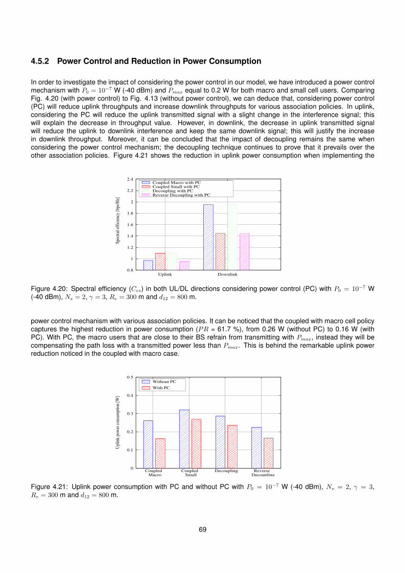
4.5.2 Power Control and Reduction in Power Consumption
In order to investigate the impact of considering the power control in our model, we have introduced a power controlmechanism with P0 = 10−7 W (-40 dBm) and Pmax equal to 0.2 W for both macro and small cell users. ComparingFig. 4.20 (with power control) to Fig. 4.13 (without power control), we can deduce that, considering power control(PC) will reduce uplink throughputs and increase downlink throughputs for various association policies. In uplink,considering the PC will reduce the uplink transmitted signal with a slight change in the interference signal; thiswill explain the decrease in throughput value. However, in downlink, the decrease in uplink transmitted signalwill reduce the uplink to downlink interference and keep the same downlink signal; this will justify the increasein downlink throughput. Moreover, it can be concluded that the impact of decoupling remains the same whenconsidering the power control mechanism; the decoupling technique continues to prove that it prevails over theother association policies. Figure 4.21 shows the reduction in uplink power consumption when implementing the
0.8
1
1.2
1.4
1.6
1.8
2
2.2
2.4
Uplink Downlink
Spe
ctra
l eff
icie
ncy
[bps
/Hz]
Coupled Macro with PCCoupled Small with PCDecoupling with PCReverse Decoupling with PC
Figure 4.20: Spectral efficiency (Ces) in both UL/DL directions considering power control (PC) with P0 = 10−7 W(-40 dBm), Ns = 2, γ = 3, Re = 300 m and d12 = 800 m.
power control mechanism with various association policies. It can be noticed that the coupled with macro cell policycaptures the highest reduction in power consumption (PR = 61.7 %), from 0.26 W (without PC) to 0.16 W (withPC). With PC, the macro users that are close to their BS refrain from transmitting with Pmax, instead they will becompensating the path loss with a transmitted power less than Pmax. This is behind the remarkable uplink powerreduction noticed in the coupled with macro case.
0
0.1
0.2
0.3
0.4
0.5
Coupled Macro
Coupled Small
Decoupling Reverse Decoupling
Upl
ink
pow
er c
onsu
mpt
ion
[W]
Without PC
With PC
Figure 4.21: Uplink power consumption with PC and without PC with P0 = 10−7 W (-40 dBm), Ns = 2, γ = 3,Re = 300 m and d12 = 800 m.
69
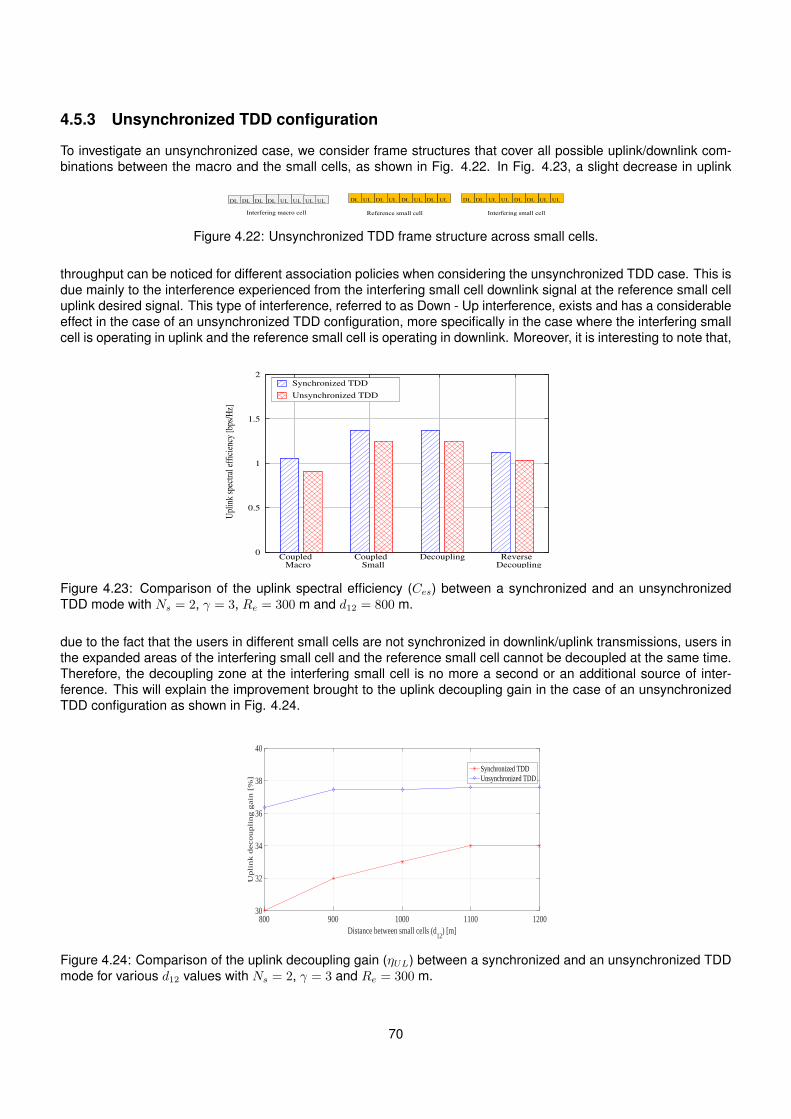
4.5.3 Unsynchronized TDD configuration
To investigate an unsynchronized case, we consider frame structures that cover all possible uplink/downlink com-binations between the macro and the small cells, as shown in Fig. 4.22. In Fig. 4.23, a slight decrease in uplink
ULDLDL
Interfering macro cell
UL
Reference small cell Interfering small cell
DLULDL UL ULDLDL ULUL ULDLDL ULDLDL ULDLULDL UL
Figure 4.22: Unsynchronized TDD frame structure across small cells.
throughput can be noticed for different association policies when considering the unsynchronized TDD case. This isdue mainly to the interference experienced from the interfering small cell downlink signal at the reference small celluplink desired signal. This type of interference, referred to as Down - Up interference, exists and has a considerableeffect in the case of an unsynchronized TDD configuration, more specifically in the case where the interfering smallcell is operating in uplink and the reference small cell is operating in downlink. Moreover, it is interesting to note that,
0
0.5
1
1.5
2
Coupled Macro
Coupled Small
Decoupling Reverse Decoupling
Upl
ink
spec
tral
eff
icie
ncy
[bps
/Hz]
Synchronized TDD
Unsynchronized TDD
Figure 4.23: Comparison of the uplink spectral efficiency (Ces) between a synchronized and an unsynchronizedTDD mode with Ns = 2, γ = 3, Re = 300 m and d12 = 800 m.
due to the fact that the users in different small cells are not synchronized in downlink/uplink transmissions, users inthe expanded areas of the interfering small cell and the reference small cell cannot be decoupled at the same time.Therefore, the decoupling zone at the interfering small cell is no more a second or an additional source of inter-ference. This will explain the improvement brought to the uplink decoupling gain in the case of an unsynchronizedTDD configuration as shown in Fig. 4.24.
Distance between small cells (d12
) [m]800 900 1000 1100 1200
Up
lin
k d
eco
up
lin
g g
ain
[%
]
30
32
34
36
38
40
Synchronized TDDUnsynchronized TDD
Figure 4.24: Comparison of the uplink decoupling gain (ηUL) between a synchronized and an unsynchronized TDDmode for various d12 values with Ns = 2, γ = 3 and Re = 300 m.
70
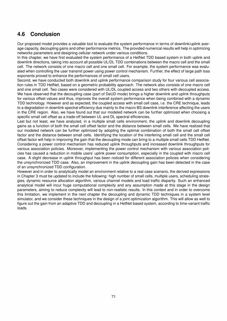
4.6 Conclusion
Our proposed model provides a valuable tool to evaluate the system performance in terms of downlink/uplink aver-age capacity, decoupling gains and other performance metrics. The provided numerical results will help in optimizingnetworks parameters and designing cellular network under various conditions.In this chapter, we have first evaluated the system performance of a HetNet TDD based system in both uplink anddownlink directions, taking into account all possible UL/DL TDD combinations between the macro cell and the smallcell. The network consists of one macro cell and one small cell. For example, the system performance was evalu-ated when controlling the user transmit power using power control mechanism. Further, the effect of large path lossexponents proved to enhance the performances of small cell users.Second, we have conducted both downlink and uplink performance comparison study for four various cell associa-tion rules in TDD HetNet, based on a geometric probability approach. The network also consists of one macro celland one small cell. Two cases were considered with UL/DL coupled access and two others with decoupled access.We have observed that the decoupling case (part of DeUD mode) brings a higher downlink and uplink throughputsfor various offset values and thus, improves the overall system performance when being combined with a dynamicTDD technology. However and as expected, the coupled access with small cell case, i.e. the CRE technique, leadsto a degradation in downlink spectral efficiency due mainly to the macro BS downlink interference affecting the usersin the CRE region. Also, we have found out that our modeled network can be further optimized when choosing aspecific small cell offset as a trade-off between UL and DL spectral efficiencies.Last but not least, we have analyzed, in a multiple small cells environment, the uplink and downlink decouplinggains as a function of both the small cell offset factor and the distance between small cells. We have realized thatour modeled network can be further optimized by adopting the optimal combination of both the small cell offsetfactor and the distance between small cells. Identifying the location of the interfering small cell and the small celloffset factor will help in improving the gain that the decoupling mode can bring to a multiple small cells TDD HetNet.Considering a power control mechanism has reduced uplink throughputs and increased downlink throughputs forvarious association policies. Moreover, implementing the power control mechanism with various association poli-cies has caused a reduction in mobile users’ uplink power consumption, especially in the coupled with macro cellcase. A slight decrease in uplink throughput has been noticed for different association policies when consideringthe unsynchronized TDD case. Also, an improvement in the uplink decoupling gain has been detected in the caseof an unsynchronized TDD configuration.However and in order to analytically model an environment relative to a real case scenario, the derived expressionsin Chapter 3 must be updated to include the following: high number of small cells, multiple users, scheduling strate-gies, dynamic resource allocation algorithm, various channel models and load traffic disparity. Such an enhancedanalytical model will incur huge computational complexity and any assumption made at this stage in the designparameters, aiming to reduce complexity will lead to non-realistic results. In this context and in order to overcomethis limitation, we implement in the next chapter the decoupling and dynamic TDD techniques in a system levelsimulator, and we consider these techniques in the design of a joint optimization algorithm. This will allow as well tofigure out the gain from an adaptive TDD and decoupling in a HetNet based system, according to time-variant trafficloads.
71

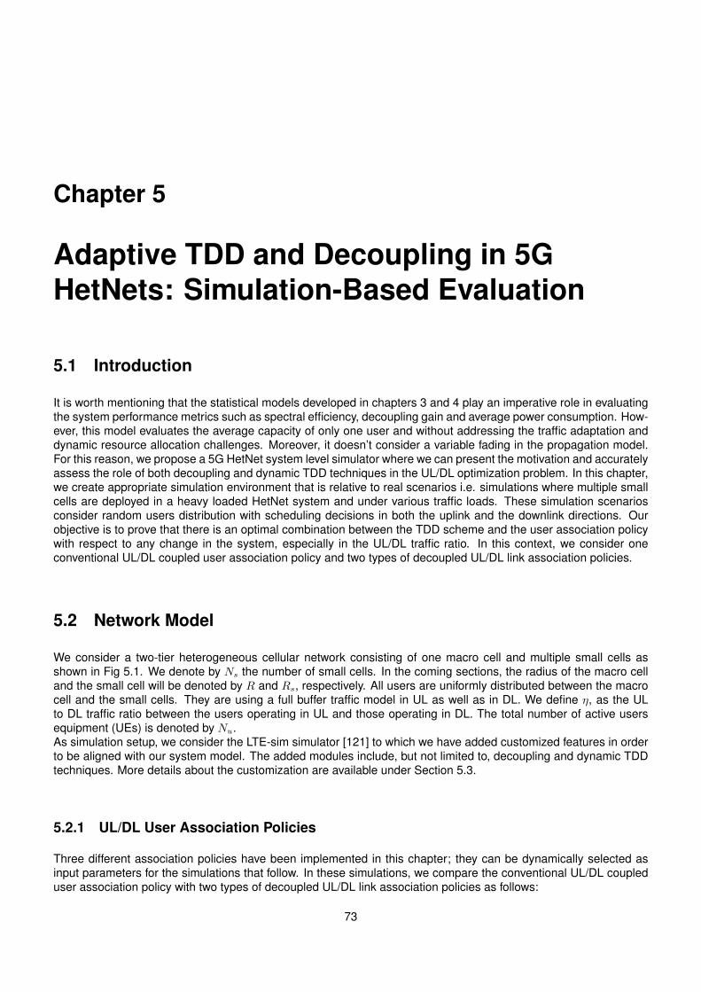
Chapter 5
Adaptive TDD and Decoupling in 5GHetNets: Simulation-Based Evaluation
5.1 Introduction
It is worth mentioning that the statistical models developed in chapters 3 and 4 play an imperative role in evaluatingthe system performance metrics such as spectral efficiency, decoupling gain and average power consumption. How-ever, this model evaluates the average capacity of only one user and without addressing the traffic adaptation anddynamic resource allocation challenges. Moreover, it doesn’t consider a variable fading in the propagation model.For this reason, we propose a 5G HetNet system level simulator where we can present the motivation and accuratelyassess the role of both decoupling and dynamic TDD techniques in the UL/DL optimization problem. In this chapter,we create appropriate simulation environment that is relative to real scenarios i.e. simulations where multiple smallcells are deployed in a heavy loaded HetNet system and under various traffic loads. These simulation scenariosconsider random users distribution with scheduling decisions in both the uplink and the downlink directions. Ourobjective is to prove that there is an optimal combination between the TDD scheme and the user association policywith respect to any change in the system, especially in the UL/DL traffic ratio. In this context, we consider oneconventional UL/DL coupled user association policy and two types of decoupled UL/DL link association policies.
5.2 Network Model
We consider a two-tier heterogeneous cellular network consisting of one macro cell and multiple small cells asshown in Fig 5.1. We denote by Ns the number of small cells. In the coming sections, the radius of the macro celland the small cell will be denoted by R and Rs, respectively. All users are uniformly distributed between the macrocell and the small cells. They are using a full buffer traffic model in UL as well as in DL. We define η, as the ULto DL traffic ratio between the users operating in UL and those operating in DL. The total number of active usersequipment (UEs) is denoted by Nu.As simulation setup, we consider the LTE-sim simulator [121] to which we have added customized features in orderto be aligned with our system model. The added modules include, but not limited to, decoupling and dynamic TDDtechniques. More details about the customization are available under Section 5.3.
5.2.1 UL/DL User Association Policies
Three different association policies have been implemented in this chapter; they can be dynamically selected asinput parameters for the simulations that follow. In these simulations, we compare the conventional UL/DL coupleduser association policy with two types of decoupled UL/DL link association policies as follows:
73
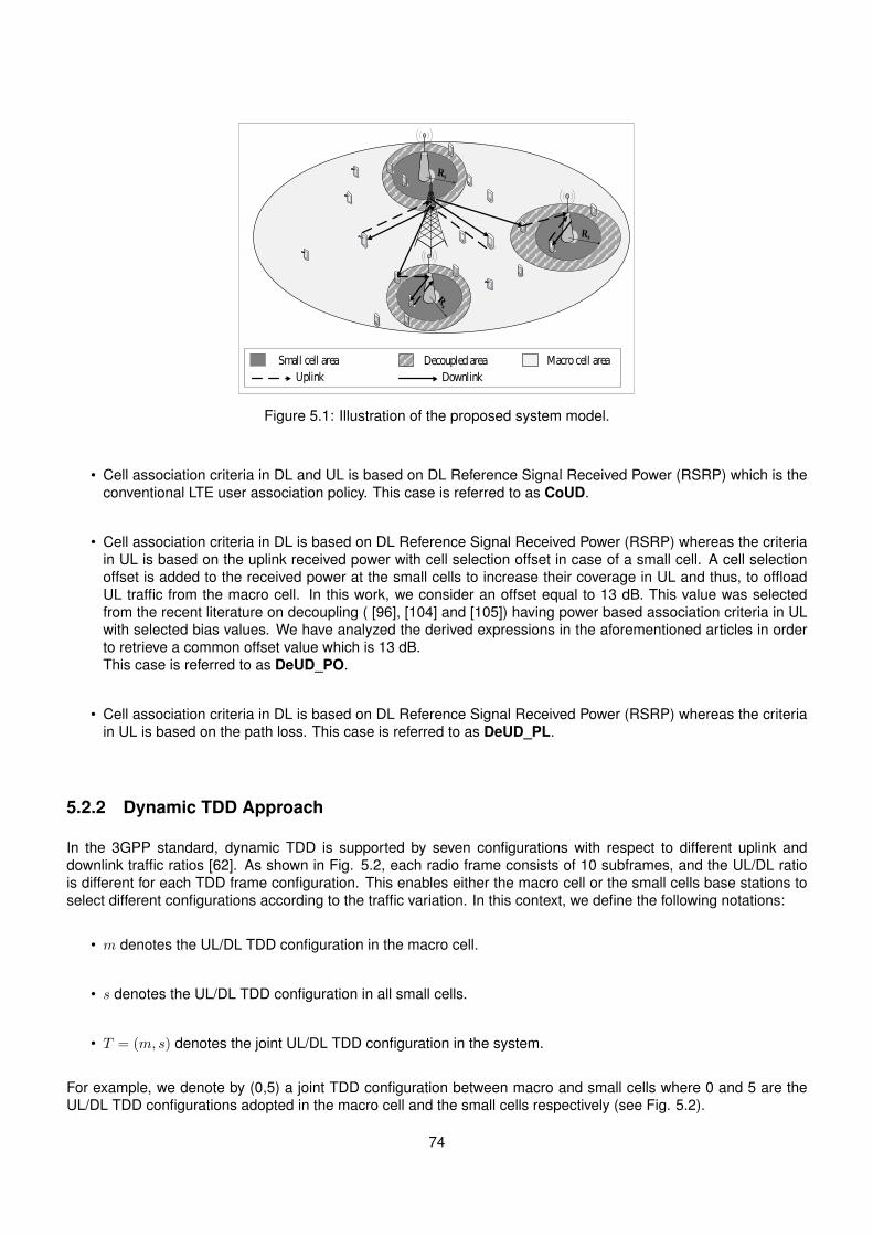
Decoupled areaSmall cell area Macro cell area
DownlinkUplink
Figure 5.1: Illustration of the proposed system model.
• Cell association criteria in DL and UL is based on DL Reference Signal Received Power (RSRP) which is theconventional LTE user association policy. This case is referred to as CoUD.
• Cell association criteria in DL is based on DL Reference Signal Received Power (RSRP) whereas the criteriain UL is based on the uplink received power with cell selection offset in case of a small cell. A cell selectionoffset is added to the received power at the small cells to increase their coverage in UL and thus, to offloadUL traffic from the macro cell. In this work, we consider an offset equal to 13 dB. This value was selectedfrom the recent literature on decoupling ( [96], [104] and [105]) having power based association criteria in ULwith selected bias values. We have analyzed the derived expressions in the aforementioned articles in orderto retrieve a common offset value which is 13 dB.This case is referred to as DeUD_PO.
• Cell association criteria in DL is based on DL Reference Signal Received Power (RSRP) whereas the criteriain UL is based on the path loss. This case is referred to as DeUD_PL.
5.2.2 Dynamic TDD Approach
In the 3GPP standard, dynamic TDD is supported by seven configurations with respect to different uplink anddownlink traffic ratios [62]. As shown in Fig. 5.2, each radio frame consists of 10 subframes, and the UL/DL ratiois different for each TDD frame configuration. This enables either the macro cell or the small cells base stations toselect different configurations according to the traffic variation. In this context, we define the following notations:
• m denotes the UL/DL TDD configuration in the macro cell.
• s denotes the UL/DL TDD configuration in all small cells.
• T = (m, s) denotes the joint UL/DL TDD configuration in the system.
For example, we denote by (0,5) a joint TDD configuration between macro and small cells where 0 and 5 are theUL/DL TDD configurations adopted in the macro cell and the small cells respectively (see Fig. 5.2).
74
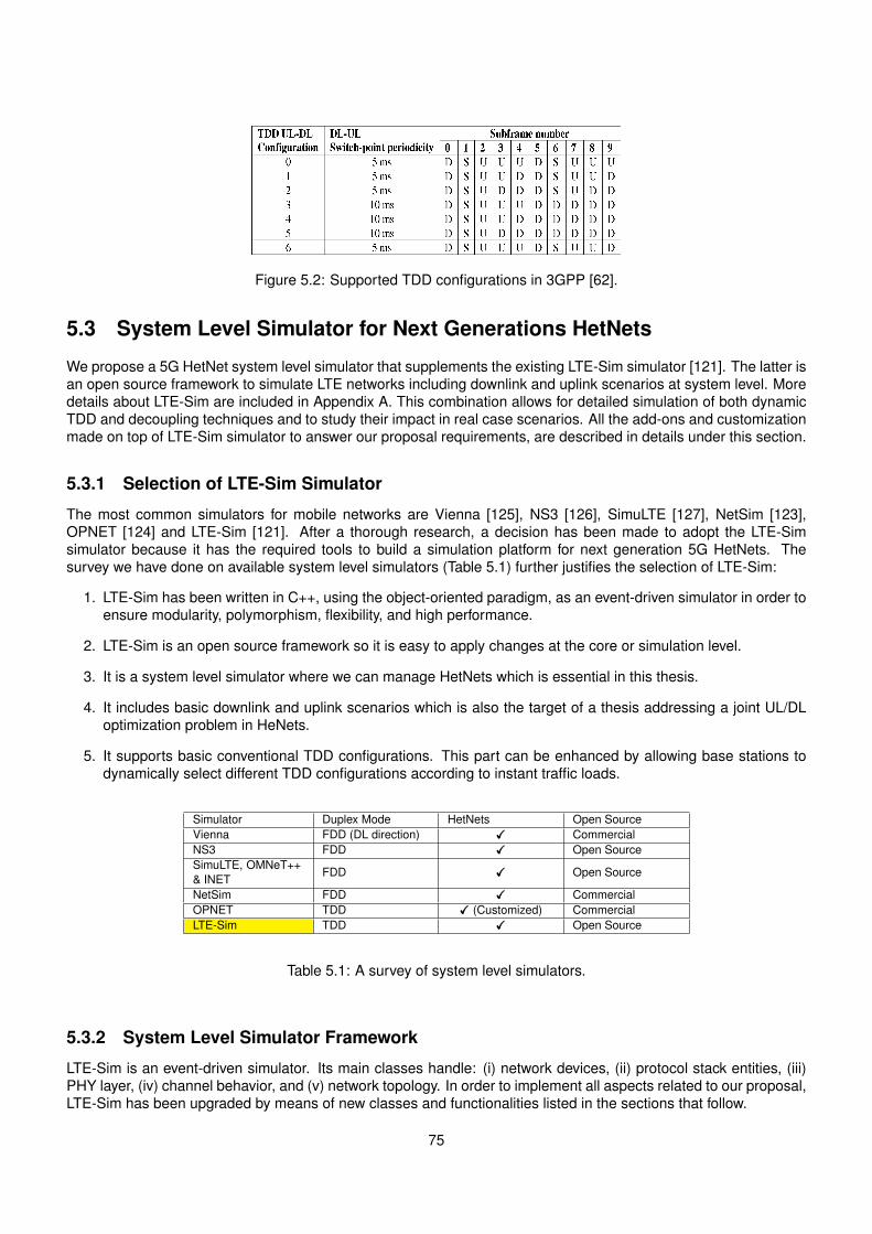
Figure 5.2: Supported TDD configurations in 3GPP [62].
5.3 System Level Simulator for Next Generations HetNets
We propose a 5G HetNet system level simulator that supplements the existing LTE-Sim simulator [121]. The latter isan open source framework to simulate LTE networks including downlink and uplink scenarios at system level. Moredetails about LTE-Sim are included in Appendix A. This combination allows for detailed simulation of both dynamicTDD and decoupling techniques and to study their impact in real case scenarios. All the add-ons and customizationmade on top of LTE-Sim simulator to answer our proposal requirements, are described in details under this section.
5.3.1 Selection of LTE-Sim Simulator
The most common simulators for mobile networks are Vienna [125], NS3 [126], SimuLTE [127], NetSim [123],OPNET [124] and LTE-Sim [121]. After a thorough research, a decision has been made to adopt the LTE-Simsimulator because it has the required tools to build a simulation platform for next generation 5G HetNets. Thesurvey we have done on available system level simulators (Table 5.1) further justifies the selection of LTE-Sim:
1. LTE-Sim has been written in C++, using the object-oriented paradigm, as an event-driven simulator in order toensure modularity, polymorphism, flexibility, and high performance.
2. LTE-Sim is an open source framework so it is easy to apply changes at the core or simulation level.
3. It is a system level simulator where we can manage HetNets which is essential in this thesis.
4. It includes basic downlink and uplink scenarios which is also the target of a thesis addressing a joint UL/DLoptimization problem in HeNets.
5. It supports basic conventional TDD configurations. This part can be enhanced by allowing base stations todynamically select different TDD configurations according to instant traffic loads.
Simulator Duplex Mode HetNets Open SourceVienna FDD (DL direction) XXX CommercialNS3 FDD XXX Open SourceSimuLTE, OMNeT++& INET
FDD XXX Open Source
NetSim FDD XXX CommercialOPNET TDD XXX (Customized) CommercialLTE-Sim TDD XXX Open Source
Table 5.1: A survey of system level simulators.
5.3.2 System Level Simulator Framework
LTE-Sim is an event-driven simulator. Its main classes handle: (i) network devices, (ii) protocol stack entities, (iii)PHY layer, (iv) channel behavior, and (v) network topology. In order to implement all aspects related to our proposal,LTE-Sim has been upgraded by means of new classes and functionalities listed in the sections that follow.
75
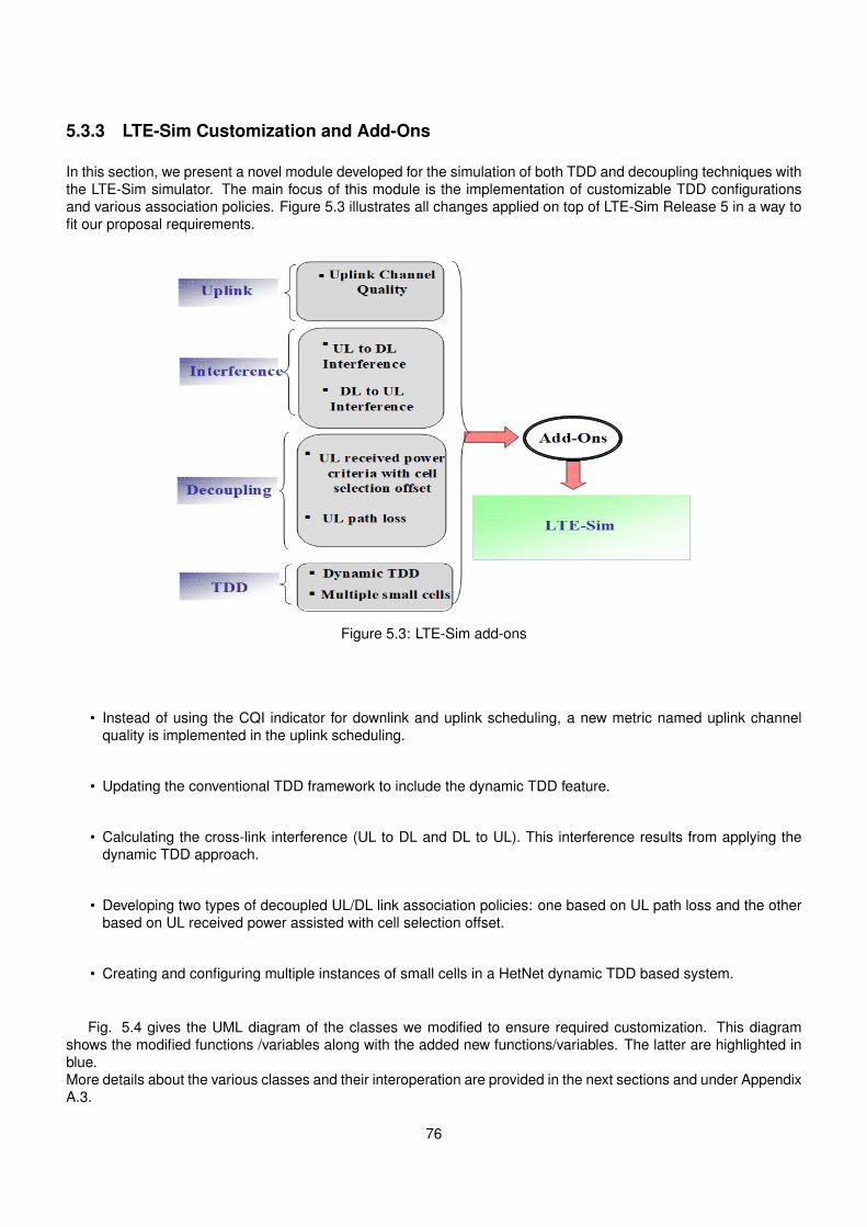
5.3.3 LTE-Sim Customization and Add-Ons
In this section, we present a novel module developed for the simulation of both TDD and decoupling techniques withthe LTE-Sim simulator. The main focus of this module is the implementation of customizable TDD configurationsand various association policies. Figure 5.3 illustrates all changes applied on top of LTE-Sim Release 5 in a way tofit our proposal requirements.
Figure 5.3: LTE-Sim add-ons
• Instead of using the CQI indicator for downlink and uplink scheduling, a new metric named uplink channelquality is implemented in the uplink scheduling.
• Updating the conventional TDD framework to include the dynamic TDD feature.
• Calculating the cross-link interference (UL to DL and DL to UL). This interference results from applying thedynamic TDD approach.
• Developing two types of decoupled UL/DL link association policies: one based on UL path loss and the otherbased on UL received power assisted with cell selection offset.
• Creating and configuring multiple instances of small cells in a HetNet dynamic TDD based system.
Fig. 5.4 gives the UML diagram of the classes we modified to ensure required customization. This diagramshows the modified functions /variables along with the added new functions/variables. The latter are highlighted inblue.More details about the various classes and their interoperation are provided in the next sections and under AppendixA.3.
76
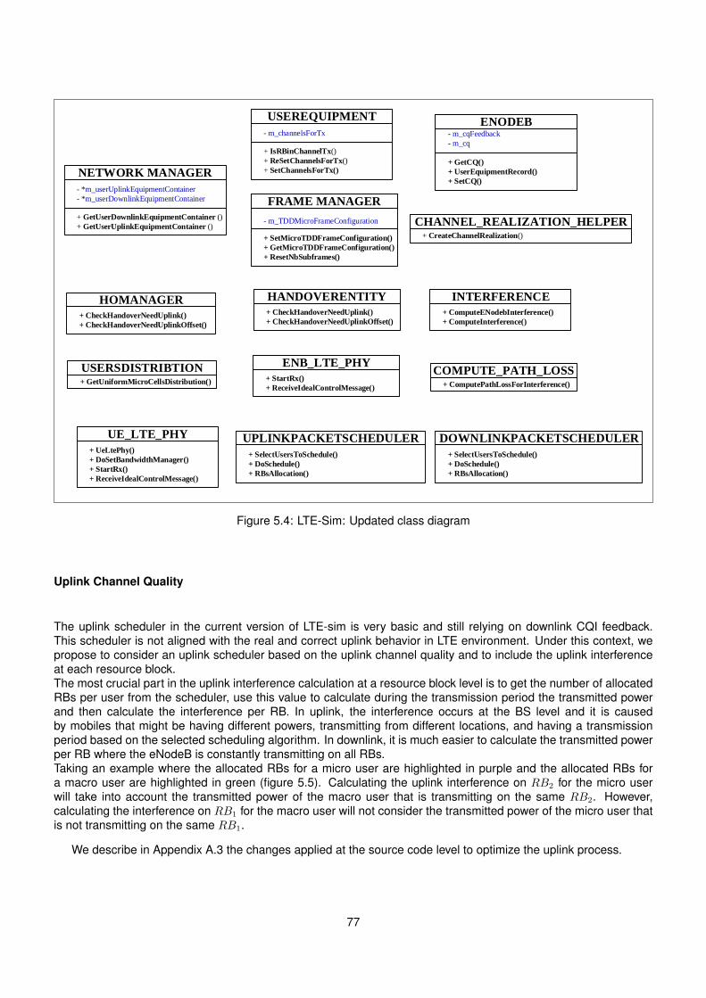
- *m_userUplinkEquipmentContainer
- *m_userDownlinkEquipmentContainer
NETWORK MANAGER
+ GetUserDownlinkEquipmentContainer ()
+ GetUserUplinkEquipmentContainer ()- m_TDDMicroFrameConfiguration
FRAME MANAGER
+ SetMicroTDDFrameConfiguration()
+ GetMicroTDDFrameConfiguration()
+ ResetNbSubframes()
HOMANAGER
+ CheckHandoverNeedUplink()
+ CheckHandoverNeedUplinkOffset()
HANDOVERENTITY
+ CheckHandoverNeedUplink()
+ CheckHandoverNeedUplinkOffset()
USERSDISTRIBTION+ GetUniformMicroCellsDistribution()
ENB_LTE_PHY
+ StartRx()
+ ReceiveIdealControlMessage()
UE_LTE_PHY
+ UeLtePhy()
+ DoSetBandwidthManager()
+ StartRx()
+ ReceiveIdealControlMessage()
UPLINKPACKETSCHEDULER
+ SelectUsersToSchedule()
+ DoSchedule()
+ RBsAllocation()
DOWNLINKPACKETSCHEDULER
+ SelectUsersToSchedule()
+ DoSchedule()
+ RBsAllocation()
COMPUTE_PATH_LOSS+ ComputePathLossForInterference()
INTERFERENCE
+ ComputeENodebInterference()
+ ComputeInterference()
CHANNEL_REALIZATION_HELPER+ CreateChannelRealization()
- m_cqFeedback
- m_cq
ENODEB
+ GetCQ()
+ UserEquipmentRecord()
+ SetCQ()
- m_channelsForTx
USEREQUIPMENT
+ IsRBinChannelTx()
+ ReSetChannelsForTx()
+ SetChannelsForTx()
Figure 5.4: LTE-Sim: Updated class diagram
Uplink Channel Quality
The uplink scheduler in the current version of LTE-sim is very basic and still relying on downlink CQI feedback.This scheduler is not aligned with the real and correct uplink behavior in LTE environment. Under this context, wepropose to consider an uplink scheduler based on the uplink channel quality and to include the uplink interferenceat each resource block.The most crucial part in the uplink interference calculation at a resource block level is to get the number of allocatedRBs per user from the scheduler, use this value to calculate during the transmission period the transmitted powerand then calculate the interference per RB. In uplink, the interference occurs at the BS level and it is causedby mobiles that might be having different powers, transmitting from different locations, and having a transmissionperiod based on the selected scheduling algorithm. In downlink, it is much easier to calculate the transmitted powerper RB where the eNodeB is constantly transmitting on all RBs.Taking an example where the allocated RBs for a micro user are highlighted in purple and the allocated RBs fora macro user are highlighted in green (figure 5.5). Calculating the uplink interference on RB2 for the micro userwill take into account the transmitted power of the macro user that is transmitting on the same RB2. However,calculating the interference on RB1 for the macro user will not consider the transmitted power of the micro user thatis not transmitting on the same RB1.
We describe in Appendix A.3 the changes applied at the source code level to optimize the uplink process.
77
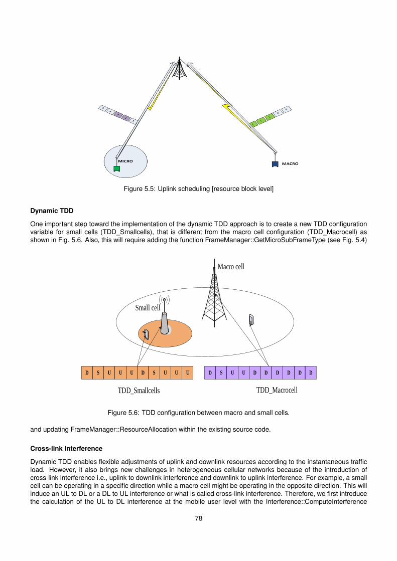
Figure 5.5: Uplink scheduling [resource block level]
Dynamic TDD
One important step toward the implementation of the dynamic TDD approach is to create a new TDD configurationvariable for small cells (TDD_Smallcells), that is different from the macro cell configuration (TDD_Macrocell) asshown in Fig. 5.6. Also, this will require adding the function FrameManager::GetMicroSubFrameType (see Fig. 5.4)
D D DU U U
Macro cell
Small cell
TDD_Smallcells TDD_Macrocell
U D DD S U DU D SS U UD
Figure 5.6: TDD configuration between macro and small cells.
and updating FrameManager::ResourceAllocation within the existing source code.
Cross-link Interference
Dynamic TDD enables flexible adjustments of uplink and downlink resources according to the instantaneous trafficload. However, it also brings new challenges in heterogeneous cellular networks because of the introduction ofcross-link interference i.e., uplink to downlink interference and downlink to uplink interference. For example, a smallcell can be operating in a specific direction while a macro cell might be operating in the opposite direction. This willinduce an UL to DL or a DL to UL interference or what is called cross-link interference. Therefore, we first introducethe calculation of the UL to DL interference at the mobile user level with the Interference::ComputeInterference
78
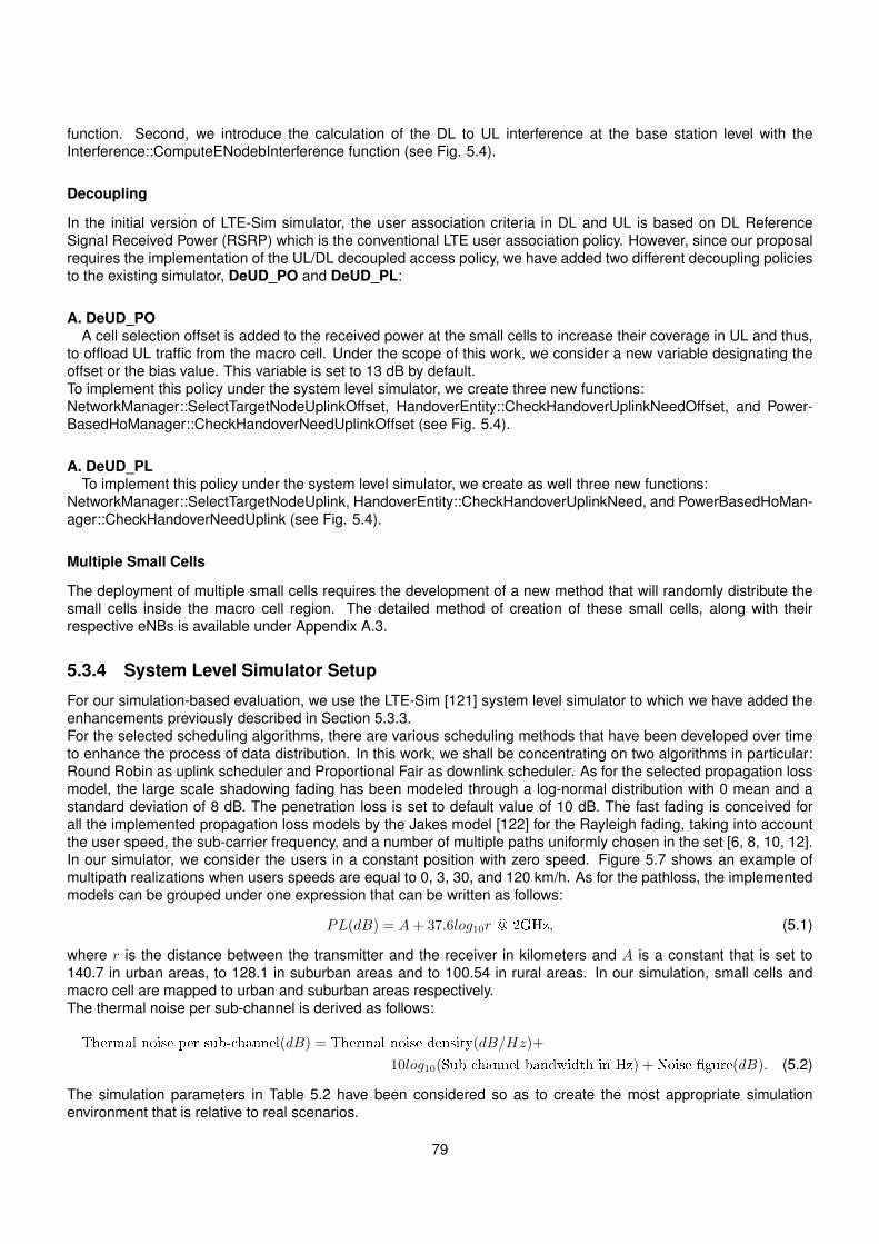
function. Second, we introduce the calculation of the DL to UL interference at the base station level with theInterference::ComputeENodebInterference function (see Fig. 5.4).
Decoupling
In the initial version of LTE-Sim simulator, the user association criteria in DL and UL is based on DL ReferenceSignal Received Power (RSRP) which is the conventional LTE user association policy. However, since our proposalrequires the implementation of the UL/DL decoupled access policy, we have added two different decoupling policiesto the existing simulator, DeUD_PO and DeUD_PL:
A. DeUD_POA cell selection offset is added to the received power at the small cells to increase their coverage in UL and thus,
to offload UL traffic from the macro cell. Under the scope of this work, we consider a new variable designating theoffset or the bias value. This variable is set to 13 dB by default.To implement this policy under the system level simulator, we create three new functions:NetworkManager::SelectTargetNodeUplinkOffset, HandoverEntity::CheckHandoverUplinkNeedOffset, and Power-BasedHoManager::CheckHandoverNeedUplinkOffset (see Fig. 5.4).
A. DeUD_PLTo implement this policy under the system level simulator, we create as well three new functions:
NetworkManager::SelectTargetNodeUplink, HandoverEntity::CheckHandoverUplinkNeed, and PowerBasedHoMan-ager::CheckHandoverNeedUplink (see Fig. 5.4).
Multiple Small Cells
The deployment of multiple small cells requires the development of a new method that will randomly distribute thesmall cells inside the macro cell region. The detailed method of creation of these small cells, along with theirrespective eNBs is available under Appendix A.3.
5.3.4 System Level Simulator Setup
For our simulation-based evaluation, we use the LTE-Sim [121] system level simulator to which we have added theenhancements previously described in Section 5.3.3.For the selected scheduling algorithms, there are various scheduling methods that have been developed over timeto enhance the process of data distribution. In this work, we shall be concentrating on two algorithms in particular:Round Robin as uplink scheduler and Proportional Fair as downlink scheduler. As for the selected propagation lossmodel, the large scale shadowing fading has been modeled through a log-normal distribution with 0 mean and astandard deviation of 8 dB. The penetration loss is set to default value of 10 dB. The fast fading is conceived forall the implemented propagation loss models by the Jakes model [122] for the Rayleigh fading, taking into accountthe user speed, the sub-carrier frequency, and a number of multiple paths uniformly chosen in the set [6, 8, 10, 12].In our simulator, we consider the users in a constant position with zero speed. Figure 5.7 shows an example ofmultipath realizations when users speeds are equal to 0, 3, 30, and 120 km/h. As for the pathloss, the implementedmodels can be grouped under one expression that can be written as follows:
PL(dB) = A+ 37.6log10r @ 2GHz, (5.1)
where r is the distance between the transmitter and the receiver in kilometers and A is a constant that is set to140.7 in urban areas, to 128.1 in suburban areas and to 100.54 in rural areas. In our simulation, small cells andmacro cell are mapped to urban and suburban areas respectively.The thermal noise per sub-channel is derived as follows:
Thermal noise per sub-channel(dB) = Thermal noise density(dB/Hz)+
10log10(Sub-channel bandwidth in Hz) +Noise �gure(dB). (5.2)
The simulation parameters in Table 5.2 have been considered so as to create the most appropriate simulationenvironment that is relative to real scenarios.
79
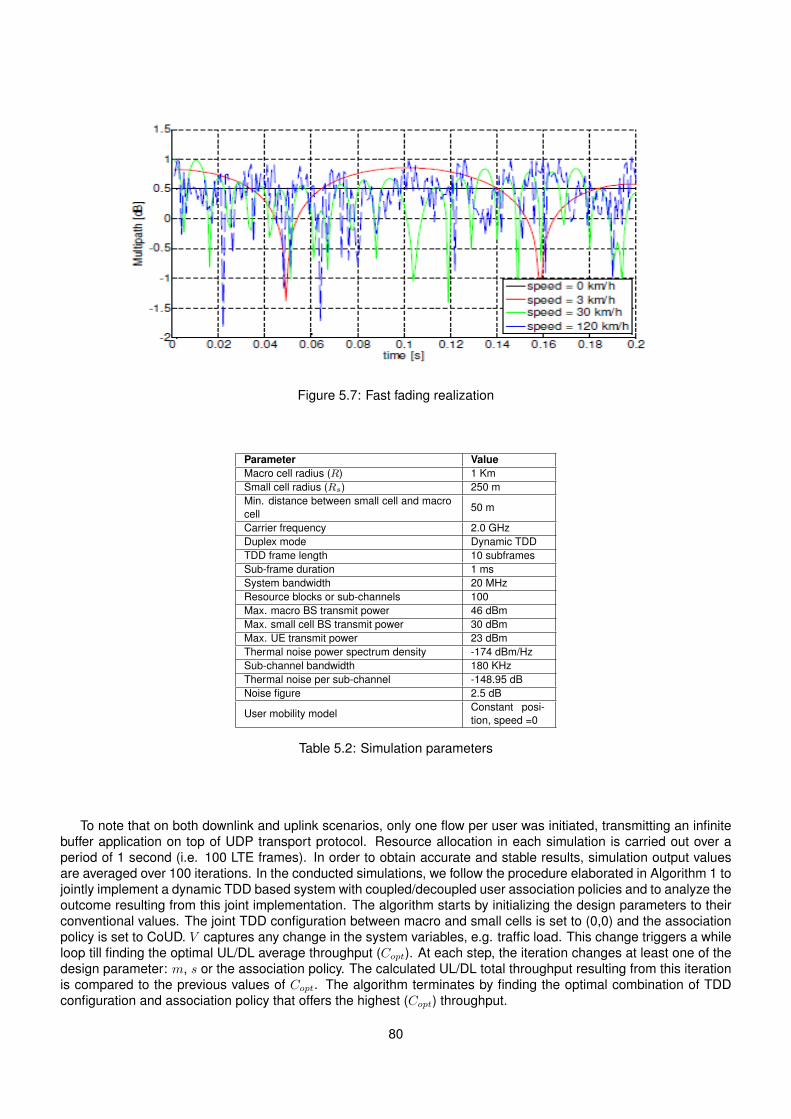
Figure 5.7: Fast fading realization
Parameter ValueMacro cell radius (R) 1 KmSmall cell radius (Rs) 250 mMin. distance between small cell and macrocell
50 m
Carrier frequency 2.0 GHzDuplex mode Dynamic TDDTDD frame length 10 subframesSub-frame duration 1 msSystem bandwidth 20 MHzResource blocks or sub-channels 100Max. macro BS transmit power 46 dBmMax. small cell BS transmit power 30 dBmMax. UE transmit power 23 dBmThermal noise power spectrum density -174 dBm/HzSub-channel bandwidth 180 KHzThermal noise per sub-channel -148.95 dBNoise figure 2.5 dB
User mobility modelConstant posi-tion, speed =0
Table 5.2: Simulation parameters
To note that on both downlink and uplink scenarios, only one flow per user was initiated, transmitting an infinitebuffer application on top of UDP transport protocol. Resource allocation in each simulation is carried out over aperiod of 1 second (i.e. 100 LTE frames). In order to obtain accurate and stable results, simulation output valuesare averaged over 100 iterations. In the conducted simulations, we follow the procedure elaborated in Algorithm 1 tojointly implement a dynamic TDD based system with coupled/decoupled user association policies and to analyze theoutcome resulting from this joint implementation. The algorithm starts by initializing the design parameters to theirconventional values. The joint TDD configuration between macro and small cells is set to (0,0) and the associationpolicy is set to CoUD. V captures any change in the system variables, e.g. traffic load. This change triggers a whileloop till finding the optimal UL/DL average throughput (Copt). At each step, the iteration changes at least one of thedesign parameter: m, s or the association policy. The calculated UL/DL total throughput resulting from this iterationis compared to the previous values of Copt. The algorithm terminates by finding the optimal combination of TDDconfiguration and association policy that offers the highest (Copt) throughput.
80
Algorithm 1 Adaptive TDD and coupled/decoupled user association policies
1: procedure SIMULATION PROCEDURE2: T=(m,s)← Joint TDD configuration3: ua← User association policy4: V ← System input variables5: Copt ← UL and DL optimal average throughput6: Tempopt ← UL and DL temporary optimal average throughput7: Copt ← Calculate(ua,(m, s), V )8: while V changes do9: for m← 0 to 6 do
10: for s← 0 to 6 do11: ua← CoUD12: Tempopt ← Calculate(ua,(m, s), V )13: if Tempopt > Copt then14: Copt ← Tempopt.15: ua← DeUD16: Tempopt ← Calculate(ua,(m, s), V )17: if Tempopt > Copt then18: Copt ← Tempopt.
5.3.5 Network Performance Metrics
In this chapter, several performance metrics are identified to be used as a means to evaluate and compare allsimulation results. We present hereafter the definition and the motivation of each of these metrics.
A. Throughput
Throughput measures the network actual data transmission rate, which can vary wildly through different areas ofa HetNet based system. While the network bandwidth measures the theoretical limit of data transfer, throughputtells how much data is actually being sent. Specifically, throughput measures the amount of data that is successfullybeing sent over a specific period or simulation time. In our simulator, we capture the total average system throughputin Mbps, including the macro cell and the small cells throughputs in both UL and DL directions.
B. Outage / Coverage Probability
A crucial aspect in the evaluation and planning of a wireless network is the effect of interference imposed onradio links. The probabilities that the throughput drops below and rises above a certain threshold are defined asoutage probability and coverage probability, respectively. The outage/coverage probability is crucial in terms ofbenchmarking the average throughput of a randomly chosen user in the network, and serves as a fundamental met-ric for network performance analysis and optimization. In our simulator, we capture the average outage probabilityof the users associated to the macro cell from one side and those attached to the small cells from the other side.
C. Throughput Percentile
In 3GPP, the cell edge user throughput is defined as the 5th percentile point of the CDF of users’ average through-put per transmission, assuming that 95% of the users are expected to achieve a certain throughput per transmissionregardless of their geographical location in the cell. If the optimization goal is to maximize the coverage, the 5th per-centile cell edge users should acquire an acceptable throughput. Similarly, the 50th and 90th percentile are definedas the 50th and 90th point of the CDF of the UE throughput respectively. They are measured to evaluate the usersthroughput inside a specific cell. In our simulator, we investigate the 5th, 50th and 90th percentile uplink throughputfor different association policies in comparison.
In order to evaluate the presented performance metrics and since the current version of the simulator provides
81
a sophisticated tracing functionality, we develop a new windows based application to analyze the LTE-Sim traces(Fig. 5.8), parse them and represent the calculated metrics under a graphical user interface.
Figure 5.8: LTE-Sim traces example
5.4 Simulation Results
In this section, we evaluate first the performance of a HetNet system adopting the conventional TDD configuration(i.e. an UL/DL fixed configuration) with coupled/decoupled association policies. Then, we will follow the procedure inAlgorithm 1 and assess the improvement brought by the joint implementation of dynamic TDD and UL/DL decoupledaccess to the system, in terms of UL and DL throughputs.
5.4.1 Coupled/Decoupled Association Policies in a Conventional TDD System
Figure 5.9 shows the evolution of UE average uplink throughput as a function of the number of small cells for variousassociation criteria with T = (0,0). We notice that the decoupling case with path loss option (DeUD_PL) outperformsCoUD and DeUD_PO cases regardless of the number of deployed small cells. This is due to the fact that users aredispersed and not centralized in one area (cell edge area or cell center area). Moreover, it came to our attentionthat CoUD case tends to progress similarly to DeUD when the number of small cells significantly increases. Thiscan be explained by the fact that, when increasing the number of small cells, the users in coupled mode are now inthe range of small cells in terms of DL signal received power, without the need to refer to the UL path loss option.
Number of small cells2 4 6 8 10 12
UE
av
erag
e u
pli
nk
th
rou
gh
pu
t [M
bp
s]
0.4
0.5
0.6
0.7
0.8
0.9
1
1.1
1.2CoUDDeUD_PO: Offset=13 dBDeUD_PL
Figure 5.9: Comparison of the UE average uplink throughput between CoUD, DeUD_PO and DeUD_PL cases vsthe number of small cells with Nu = 100, η = 0 dB and T = (0,0) (conventional TDD).
82
Figure 5.10 depicts the 5th percentile uplink throughput in a conventional TDD HetNet under various small cellsdensity. It can be observed that the DeUD_PL case prevails over the DeUD_PO case when deploying two to foursmall cells, however and after adding increasingly more small cells, we notice a drastic change in the behavior ofboth cases. The DeUD_PO case outperforms the DeUD_PL for dense small cells networks i.e. when number of de-ployed small cells is greater than four. This is due to the fact that, when adding more small cells, the cell edge userswill be more subject to harmful interference from close macro users. Consequently, and in order to mitigate the ULinterference caused by the macro users, the path loss association policy is no more able to do the job. Instead,applying the association policy that extends the small cell coverage by adding a specific bias i.e. the DeUD_POpolicy will reduce the UL interference and thus, improve the 5th percentile uplink throughput.
Number of small cells2 4 6 8 10 12
5th
perc
enti
le u
pli
nk t
hro
ughput
[Mbps]
0.02
0.04
0.06
0.08
0.1
0.12DeUD_PO: Offset=13 dBDeUD_PL
Figure 5.10: 5th percentile uplink throughput comparison between DeUD_PO and DeUD_PL cases vs the numberof small cells with Nu = 100, η = 0 dB and T = (0,0) (conventional TDD).
Figure 5.11 shows the 5th, 50th and 90th percentile uplink throughput for the three association policies in aHetNet system with 12 small cells. We can observe that the 5th percentile uplink throughput in the DeUD_PO caseis increased by 37.5 % compared to the CoUD case and by more than 400 % compared to the DeUD_PL. Thesmall cell expansion caused by the DeUD_PO plays an imperative role in decreasing the level of UL interference byattaching the macro users to the nearest small cell. This explains the improvement in 5th percentile uplink throughputbrought by the DeUD_PO case to the cell edge users. As for the 50th percentile uplink throughput, we notice thatthe DeUD_PO case outperforms both the CoUD and DeUD_PL cases by 120 % and 41 % respectively. Note thatthe gains in the 5th and 50th percentile are resulting from the higher coverage of the small cells in the DeUD_POcase with an offset equal to 13 dB. Looking at the 90th percentile UL throughput, we can see that the DeUD_PLcase achieves the highest throughput which can be explained by the fact that small cells serve less users than theDeUD_PO case so these users get a higher throughput but at the expense of the 5th and 50th percentile users.
Figure 5.12 captures the average outage probability of the users associated to the macro cell from one side andthose attached to the small cells from the other side. In this work, we define the outage probability in one cell asthe percentage of users that fail to reach the minimum throughput demand (considered as equal to 250 Kbps) outof the total number of users attached to that cell. As expected, it can be noticed that the macro cell has a very highoutage rate (more than 80 %) in the coupled CoUD case. This is basically due to the fact that the macro cell isvery congested in the UL because of the adopted association policy that is based on the downlink received power.Hence, macro cell BS won’t have enough resources to serve all of its associated users with a high throughput level.However, in the decoupled case, users are distributed more evenly between the macro and the small cells. This isreflected more obviously in the DeUD_PO case where the macro cell reaches an outage probability of 37 % andthe small cells achieve an average outage rate of 40 %. In this case, macro users who used to suffer from lowthroughput are moved to the edge of the small cells, causing a state of evenness in terms of outage probabilitybetween macro cell and small cells.
Table 5.3 shows the average number of users per cell where we calculate the average for the macro cell and thesmall cells separately for a total number of 200 users for all cases. Note that we consider in this scenario a total offour randomly distributed small cells. This table shows how most of the users are connected to the macro cell andhow the small cells are under-utilized in the conventional CoUD case. On the other hand, the users in the DeUD_PL
83
0
0.5
1
1.5
2
2.5
3
5th
percentile 50th
percentile 90th
percentile
Upl
ink
thro
ughp
ut [
Mbp
s]
CoUD
DeUD-PO
DeUD-PL
Figure 5.11: 5th, 50th and 90th percentile uplink throughput comparison of CoUD, DeUD_PO and DeUD_PL caseswith Nu = 100, Ns = 12, η = 0 dB and T = (0,0) (conventional TDD).
0
20
40
60
80
100
CoUD DeUD-PO DeUD-PL
Out
age
prob
abil
ity
[%]
Macro cell Small cell
Figure 5.12: Outage probability in macro and small cells between CoUD, DeUD_PO and DeUD_PL cases withNu = 100, Ns = 4, η = 0 dB and T = (0,0) (conventional TDD).
case are distributed in a more homogeneous way among the macro cell and the small cells, which ensures muchmore efficient resource utilization.
Macro cell Small cellDeUD_PL 126 25CoUD 146 5
Table 5.3: Average number of users per node (macro and small cells) for the CoUD and DeUD_PL cases.
Figure 5.13 shows the comparison between both CoUD and DeUD_PL cases under various small cell downlinktransmitted powers. It can be observed that the DeUD_PL outperforms the CoUD case, in terms of total averageUL throughput irrespective of the small cell downlink power. This is due mainly to the fact that the decoupling policyimproves the average UL throughput of both macro and small cell users, whereas the coupled policy improves theUL throughput of small cell edge users. Increasing the DL signal received power will extend the small cell uplinkcoverage in the CoUD case where the UL association citeria is based on DL received power. This will offload themacro cell, mitigate the uplink interference experienced from the macro users at the small cell BS and thus, improvethe small cell users uplink throughput. However, in the DeUD_PL case, the UL association criteria is based on theuplink path loss and thus, not affected by the change in the small cell transmit power. This will justify the steadyvalue of the UL throughput shown in Fig. 5.13.
84
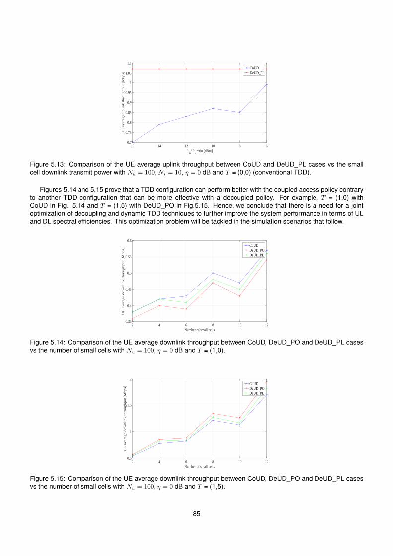
Pm
/ Ps ratio [dBm]
6810121416
UE
aver
age
upli
nk t
hro
ughput
[Mbps]
0.7
0.75
0.8
0.85
0.9
0.95
1
1.05
1.1CoUDDeUD_PL
Figure 5.13: Comparison of the UE average uplink throughput between CoUD and DeUD_PL cases vs the smallcell downlink transmit power with Nu = 100, Ns = 10, η = 0 dB and T = (0,0) (conventional TDD).
Figures 5.14 and 5.15 prove that a TDD configuration can perform better with the coupled access policy contraryto another TDD configuration that can be more effective with a decoupled policy. For example, T = (1,0) withCoUD in Fig. 5.14 and T = (1,5) with DeUD_PO in Fig.5.15. Hence, we conclude that there is a need for a jointoptimization of decoupling and dynamic TDD techniques to further improve the system performance in terms of ULand DL spectral efficiencies. This optimization problem will be tackled in the simulation scenarios that follow.
Number of small cells2 4 6 8 10 12
UE
aver
age
dow
nli
nk t
hro
ughput
[Mbps]
0.35
0.4
0.45
0.5
0.55
0.6CoUDDeUD_PODeUD_PL
Figure 5.14: Comparison of the UE average downlink throughput between CoUD, DeUD_PO and DeUD_PL casesvs the number of small cells with Nu = 100, η = 0 dB and T = (1,0).
Number of small cells2 4 6 8 10 12
UE
aver
age
dow
nli
nk t
hro
ughput
[Mbps]
0.5
1
1.5
2CoUDDeUD_PODeUD_PL
Figure 5.15: Comparison of the UE average downlink throughput between CoUD, DeUD_PO and DeUD_PL casesvs the number of small cells with Nu = 100, η = 0 dB and T = (1,5).
85
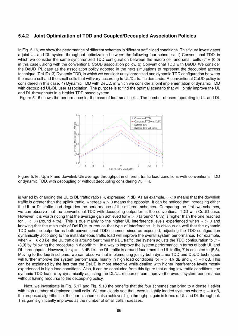
5.4.2 Joint Optimization of TDD and Coupled/Decoupled Association Policies
In Fig. 5.16, we show the performance of different schemes in different traffic load conditions. This figure investigatesa joint UL and DL system throughput optimization between the following four schemes: 1) Conventional TDD, inwhich we consider the same synchronized TDD configuration between the macro cell and small cells (T = (0,0)in this case), along with the conventional CoUD association policy. 2) Conventional TDD with DeUD. We considerthe DeUD_PL case as the association policy adopted in the next simulations to represent the decoupled accesstechnique (DeUD). 3) Dynamic TDD, in which we consider unsynchronized and dynamic TDD configuration betweenthe macro cell and the small cells that will vary according to UL/DL traffic demands. A conventional CoUD policy isconsidered in this case. 4) Dynamic TDD with DeUD, in which we consider a joint implementation of dynamic TDDwith decoupled UL/DL user association. The purpose is to find the optimal scenario that will jointly improve the ULand DL throughputs in a HetNet TDD based system.Figure 5.16 shows the performance for the case of four small cells. The number of users operating in UL and DL
UL-to-DL traffic ratio (η) [dB]-7 -6 -4.8 -3 0 3 4.8 6 7
UE
av
era
ge t
hro
ug
hp
ut
[Mb
ps]
0.1
0.2
0.3
0.4
0.5
0.6Conventional TDDConventional TDD with DeUDDynamic TDDDynamic TDD with DeUD
Figure 5.16: Uplink and downlink UE average throughput in different traffic load conditions with conventional TDDor dynamic TDD, with decoupling or without decoupling considering Ns = 4.
is varied by changing the UL to DL traffic ratio (η), expressed in dB. As an example, η < 0 means that the downlinktraffic is greater than the uplink traffic, whereas η > 0 means the opposite. It can be noticed that increasing eitherthe UL or DL traffic load degrades the performance of the different schemes. Comparing the first two schemes,we can observe that the conventional TDD with decoupling outperforms the conventional TDD with CoUD case.However, it is worth noting that the average gain achieved for η > 0 (around 16 %) is higher than the one reachedfor η < 0 (around 4 %). This is due mainly to the higher UL interference levels experienced when η > 0 andknowing that the main role of DeUD is to reduce that type of interference. It is obvious as well that the dynamicTDD scheme outperforms both conventional TDD schemes since as expected, adjusting the TDD configurationdynamically according to the instantaneous traffic load will improve the overall system performance. For example,when η = 6 dB i.e. the UL traffic is around four times the DL traffic, the system adjusts the TDD configuration to T =(3,3) by following the procedure in Algorithm 1 in a way to improve the system performance in terms of both UL andDL throughputs. However, for η = −6 dB i.e. the DL traffic is around four times the UL traffic, T is adjusted to (5,5).Moving to the fourth scheme, we can observe that implementing jointly both dynamic TDD and DeUD techniqueswill further improve the system performance, mainly in high load conditions for η > 4.8 dB and η < −3 dB. Thiscan be explained by the fact that the DeUD is more effective while dealing with higher interference levels mostlyexperienced in high load conditions. Also, it can be concluded from this figure that during low traffic conditions, thedynamic TDD feature by dynamically adjusting the DL/UL resources can improve the overall system performancewithout having recourse to the decoupling policy.
Next, we investigate in Fig. 5.17 and Fig. 5.18 the benefits that the four schemes can bring to a dense HetNetwith high number of deployed small cells. We can clearly see that, even in lightly loaded systems where η = 0 dB,the proposed algorithm i.e. the fourth scheme, also achieves high throughput gain in terms of UL and DL throughput.This gain significantly improves as the number of small cells increases.
86
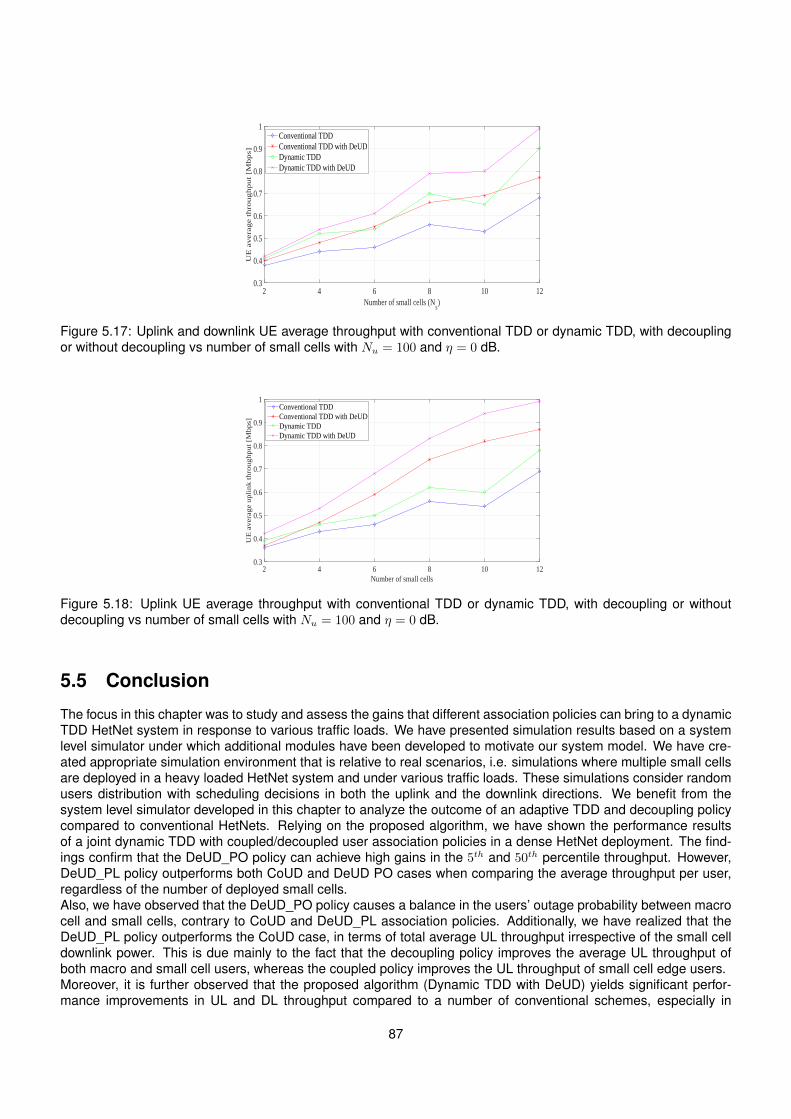
Number of small cells (Ns)
2 4 6 8 10 12
UE
av
era
ge t
hro
ug
hp
ut
[Mb
ps]
0.3
0.4
0.5
0.6
0.7
0.8
0.9
1Conventional TDDConventional TDD with DeUDDynamic TDDDynamic TDD with DeUD
Figure 5.17: Uplink and downlink UE average throughput with conventional TDD or dynamic TDD, with decouplingor without decoupling vs number of small cells with Nu = 100 and η = 0 dB.
Number of small cells2 4 6 8 10 12
UE
aver
age
upli
nk t
hro
ughput
[Mbps]
0.3
0.4
0.5
0.6
0.7
0.8
0.9
1Conventional TDDConventional TDD with DeUDDynamic TDDDynamic TDD with DeUD
Figure 5.18: Uplink UE average throughput with conventional TDD or dynamic TDD, with decoupling or withoutdecoupling vs number of small cells with Nu = 100 and η = 0 dB.
5.5 Conclusion
The focus in this chapter was to study and assess the gains that different association policies can bring to a dynamicTDD HetNet system in response to various traffic loads. We have presented simulation results based on a systemlevel simulator under which additional modules have been developed to motivate our system model. We have cre-ated appropriate simulation environment that is relative to real scenarios, i.e. simulations where multiple small cellsare deployed in a heavy loaded HetNet system and under various traffic loads. These simulations consider randomusers distribution with scheduling decisions in both the uplink and the downlink directions. We benefit from thesystem level simulator developed in this chapter to analyze the outcome of an adaptive TDD and decoupling policycompared to conventional HetNets. Relying on the proposed algorithm, we have shown the performance resultsof a joint dynamic TDD with coupled/decoupled user association policies in a dense HetNet deployment. The find-ings confirm that the DeUD_PO policy can achieve high gains in the 5th and 50th percentile throughput. However,DeUD_PL policy outperforms both CoUD and DeUD PO cases when comparing the average throughput per user,regardless of the number of deployed small cells.Also, we have observed that the DeUD_PO policy causes a balance in the users’ outage probability between macrocell and small cells, contrary to CoUD and DeUD_PL association policies. Additionally, we have realized that theDeUD_PL policy outperforms the CoUD case, in terms of total average UL throughput irrespective of the small celldownlink power. This is due mainly to the fact that the decoupling policy improves the average UL throughput ofboth macro and small cell users, whereas the coupled policy improves the UL throughput of small cell edge users.Moreover, it is further observed that the proposed algorithm (Dynamic TDD with DeUD) yields significant perfor-mance improvements in UL and DL throughput compared to a number of conventional schemes, especially in
87
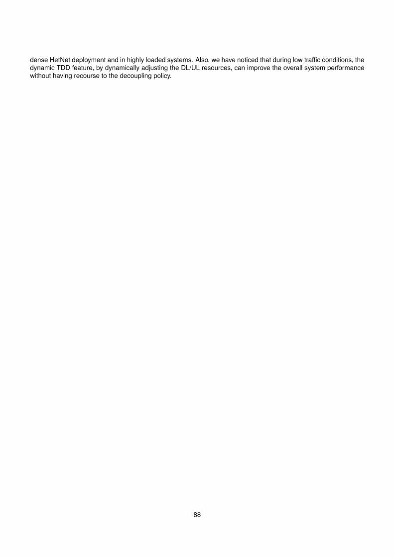
dense HetNet deployment and in highly loaded systems. Also, we have noticed that during low traffic conditions, thedynamic TDD feature, by dynamically adjusting the DL/UL resources, can improve the overall system performancewithout having recourse to the decoupling policy.
88
Chapter 6
Conclusion
In this chapter, we summarize the conclusions that we have drawn from this research, and we provide directions forfuture work.
6.1 Summary of Conclusions
This thesis addresses the challenge of integrating both TDD and uplink / downlink decoupling techniques into thesame model as a first step and to integrate them into the same simulator as a second step.Developing a statistical model for a given cellular system plays an imperative role in the design and analysis ofthat wireless cellular system. In our case, it offers a simple analysis tool to assess a given TDD/Decoupling-basedHetNet deployment. The analytical formulas provide relevant insights about network performance without the needfor time consuming Monte-Carlo Simulations. Our proposed tool is also useful for network designers who can use itto determine the range of deployment parameters given a target QoS.Therefore, and in order to meet the first thesis objective and evaluate the system performance when implementinga dynamic TDD mechanism associated with uplink / downlink decoupling, we have developed a statistical andanalytical framework that was segregated into three main sections:
• TDD Statistical Model in a Single Small Cell Environment: We have proposed an uplink and a downlinkinter-cell interference model for a dynamic TDD HetNet system considering various distance distributions. Wehave considered a network consisting of one macro cell and one small cell. We have first derived an analyticalexpression for the distribution of the interfering distance considering all possible interference scenarios thatcould occur in TDD-based networks while taking into account the harmful impact of interference. Secondly,based on the latter result, we have derived the distribution and moment generating function (MGF) of theuplink and downlink inter-cell interference. Same has been applied to the location of the reference small celluser and thus, to the distribution of the desired signal. Finally, we have built on the derived expressions forinterference and desired signal to analyze the average capacity of the reference cell in both uplink and down-link transmissions. The proposed model provides a valuable tool to evaluate the system performance in termsof downlink/uplink average capacity. The provided numerical results help in optimizing the design parametersunder various conditions. For example, the system performance was evaluated when controlling the macrouser transmission power. Further, the effect of large path loss exponents proved to enhance the performancesof small cell users.Monte-Carlo simulation results have been provided to demonstrate the accuracy of the derived analytical ex-pressions, including 95% confidence intervals of disparity measures. When evaluating the capacity expressionover 4 TDD sub frames, the execution time was found to be reduced by more than 50% compared to the timerequired to run 10 000 Monte-Carlo simulations over the same period.
• Modeling of Various Association Policies in a Single Small Cell Environment: We have conducted bothdownlink and uplink performance comparison study for four various cell association rules in TDD HetNet,based on a geometric probability approach. The network was consisting of one macro cell and one small cell.Two cases were considered with UL/DL coupled access and two others with decoupled access. This sectioncomplements the previous one by modeling the decoupling technique on top of the TDD HetNet model. Taking
89
all possible TDD subframes combinations between the macro and small cells, four coupled and decoupled cellassociations strategies have been investigated in details. This study provides more complete insights intothe benefits of decoupling mode in different network deployments with multiple input requirements. We haveobserved that the decoupling case brings greater benefits in the uplink and maintains the same improvementin the downlink for various offset values and thus, improves the overall system performance when being com-bined with a dynamic TDD technology. The same improvement in UL has been observed for the coupledaccess with small cell case. However and as expected, we have noticed that the coupled access with smallcell case, i.e. the CRE technique, leads to a degradation in downlink spectral efficiency due mainly to themacro BS downlink interference affecting the users in the CRE region. As for the reverse decoupling case, wehave captured a degradation in spectral efficiency for both UL and DL directions. On another note, we havefound out that our modeled network can be further optimized when choosing a specific small cell offset as atrade-off between UL and DL spectral efficiencies.
• Joint Modeling of TDD and Decoupling in Multiple Small Cells Environment: We have developed a jointTDD and DeUD statistical model with multiple small cells deployment. This study was based on a geometricprobability approach and considered the modeling of both cross-tier and co-tier interferences, in addition tothe average user spectral efficiency. The cross-tier interference is the interference incurred at one tier (ref-erence small cell) arising from the other tier (macro cell), whereas the co-tier interference is the interferenceincurred at the reference small cell arising from other small cells. We have analyzed, in a multiple small cellsenvironment, the uplink and downlink decoupling gains as a function of both the small cell offset factor andthe distance between small cells. Uplink power control have been added as well to the developed model.This mechanism was based on the open-loop power control strategy standardized in 3GPP LTE. Moreover,the developed statistical model has been adapted to consider an unsynchronized TDD configuration acrosssmall cells, in addition to the initial synchronized TDD configuration. Monte-Carlo simulations results havebeen presented to validate the accuracy of this model. Confidence intervals are derived for a sample mean,using the sample data values themselves. In this case, the computational time for running 1 000 000 Monte-Carlo simulations was given by 4 570 seconds which is significantly larger, when compared to the analyticalexpression evaluation time. This explained the strong need for an analytical model as a replacement for thetime consuming Monte-Carlo simulations, especially in multiple small cells environments.Regarding our findings, we have observed that the decoupling case brings higher uplink and downlink through-puts for various offset values. Furthermore, we have realized that our modeled network can be further opti-mized by adopting the optimal combination of both the small cell offset factor and the distance between smallcells. Identifying the location of the small cell interferer and the small cell offset factor will help in improvingthe gain that the decoupling mode can bring to a multiple small cells TDD HetNet. Considering a power con-trol mechanism has reduced uplink throughputs and increased downlink throughputs for various associationpolicies. Moreover, implementing the power control mechanism with various association policies has causeda reduction in mobile users’ uplink power consumption, especially in the coupled with macro cell case. Aslight decrease in uplink throughput has been noticed for different association policies when considering theunsynchronized TDD case. Also, an improvement in the uplink decoupling gain has been detected in the caseof an unsynchronized TDD configuration.
It is worth mentioning that the proposed model plays an imperative role in evaluating the system performancemetrics such as spectral efficiency, decoupling gain and average power consumption. However, this model eval-uates the average capacity of only one user and without addressing the traffic adaptation and dynamic resourceallocation challenges. Also, it doesn’t consider a variable slow and fast fading. Including these enhancements inour model will incur huge computational complexity and any assumption made at this stage in the design parame-ters, aiming to reduce model complexity will lead to non-realistic results. For this reason, we have implemented a5G HetNet system level simulator that supplements an existing LTE simulator. By this implementation, we will beanswering the second thesis objective and discovering the benefits of an adaptive TDD and decoupling comparedto conventional HetNets. We have created appropriate simulation environment that is relative to real scenarios i.e.simulations where multiple small cells are deployed in a heavy loaded HetNet system and under various traffic loads.These simulation scenarios consider random users distribution with scheduling decisions in both the uplink and thedownlink directions. Our objective was to prove that there is an optimal combination between both the macro celland the small cells TDD configurations from one side and the decoupling association with its various parametersfrom the other side, and this with respect to any change in the system, especially in the UL/DL traffic ratio:
90
• Adaptive TDD and Decoupling in 5G HetNets: Simulation-Based Evaluation: We have presented sim-ulation results based on a system level simulator under which additional modules have been developed tomotivate our system model. Relying on the proposed algorithm, we have shown the performance results ofa joint dynamic TDD with coupled/decoupled user association policies in a dense HetNet deployment. Theimplemented association policies are as follows:
– Cell association criteria in DL and UL is based on DL Reference Signal Received Power (RSRP) whichis the conventional LTE user association policy. This case is referred to as CoUD.
– Cell association criteria in DL is based on DL Reference Signal Received Power (RSRP) whereas thecriteria in UL is based on the uplink received power with cell selection offset in case of a small cell. Thiscase is referred to as DeUD_PO.
– Cell association criteria in DL is based on DL Reference Signal Received Power (RSRP) whereas thecriteria in UL is based on the path loss. This case is referred to as DeUD_PL.
The findings confirm that the DeUD_PO policy can achieve high gains in the 5th and 50th percentile through-put. However, DeUD_PL policy outperforms both CoUD and DeUD PO cases when comparing the averagethroughput per user, regardless of the number of deployed small cells. Also, we have observed that theDeUD_PO policy causes a balance in the users’ outage probability between macro cell and small cells, con-trary to CoUD and DeUD_PL association policies. Additionally, we have realized that the DeUD_PL policyoutperforms the CoUD case, in terms of total average UL throughput irrespective of the small cell downlinkpower. This is due mainly to the fact that the decoupling policy improves the average UL throughput of bothmacro and small cell users, whereas the coupled policy improves the UL throughput of small cell edge users.Findings confirm as well, that in the conventional CoUD case, most of the users are connected to the macrocell and the small cells are under-utilized. On the other hand, the users in the DeUD_PL case appear to bedistributed in a more homogeneous way among the macro cell and the small cells, which ensures much moreefficient resource utilization.
Moreover, it has been further observed that the proposed algorithm (Dynamic TDD with DeUD_PL) yields sig-nificant performance improvements in UL and DL throughput compared to a number of conventional schemes,especially in dense HetNet deployment and in highly loaded systems. This can be explained by the fact thatthe DeUD is more effective while dealing with higher interference levels mostly experienced in high load con-ditions. Also, we have noticed that during low traffic conditions, the dynamic TDD feature by dynamicallyadjusting the DL/UL resources can improve the overall system performance without adopting the decouplingpolicy.
6.2 Future Directions
We expose hereafter the future perspectives of the work in subsections 6.2.1, and 6.2.2, exposing short and longterm perspectives respectively.
6.2.1 Short Term Perspectives
For short term perspectives, we propose to consider non-uniform users distribution including the case where theusers can be present in the same place at the exact same time. Another possible extension is to consider variouscomposite fading channel models in both macro and small cells and thus, incorporate new design parametersin the developed model. The derived expressions can be also considered to evaluate other important networkperformance metrics such as network outage and average user fairness, numerically. Moreover, a future work canfocus on studying the network architectural and design changes that would enable the decoupling of UL and DLand which includes signaling and radio access protocols. This future work should outline the architectural changesrequired to facilitate the decoupled UL/DL. Based on a 3GPP architecture, several different degrees of decouplingwere proposed which mainly differ in the rigor of decoupling and the chosen anchor points in the RAN/core. Asolution can be with the centralized C-RAN technology that could be considered to gather all signaling informationin UL and DL from different base stations, in a centralized cloud ready to be shared with users associated withdifferent base stations.Further, combining the decoupling approach with other emerging paradigms, such as COMP, mmWave, D2D andMassive MU-MIMO, would be interesting items for future work. For example, massive MIMO technique introduces
91
either diversity or spatial multiplexing gain, improving energy and spectral efficiencies, and deriving more powersavings. As for the COMP technique, it is the key technique to improve the cell-edge throughput and/or systemthroughput in a HetNet based system.
6.2.2 Long Term Perspectives
As for long term perspectives, it is paramount to investigate the performance of the decoupling mode in 5G TDDsystems with hybrid HetNet deployment, where mmWave small cells (for example) are supposed to be deployed asan overlay to traditional sub-6GHz macro cells. This inter-band connectivity in 5G networks between two differentradio technologies (RAT) has been clearly described in 3GPP Release 16. As an example, a mobile user hosting avideo streaming session which generally requires a high downlink throughput, will be associated in DL to a mmwaveBS that offers a large bandwidth and thus a high throughput. However in UL, the mobile user suffering from a trans-mitted signal power limitation will be associated to a low frequency LTE BS to compensate and increase its uplinkcoverage.Additionally, resorting to learning techniques to dynamically decide the best combination between the TDD schemeand the user association policy and this adapting to dynamic traffic load variations, would also be an interesting fol-low up work. Also, these learning algorithms should as well dynamically decide which procedure to adopt regardingthe rate of deployment or change of each technique. For example, the association process for both UL and DL canbe performed in a slower rate compared to the change in TDD reconfiguration rate.
92
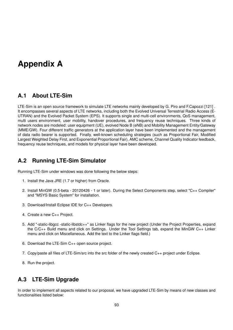
Appendix A
A.1 About LTE-Sim
LTE-Sim is an open source framework to simulate LTE networks mainly developed by G. Piro and F.Capozzi [121] .It encompasses several aspects of LTE networks, including both the Evolved Universal Terrestrial Radio Access (E-UTRAN) and the Evolved Packet System (EPS). It supports single and multi-cell environments, QoS management,multi users environment, user mobility, handover procedures, and frequency reuse techniques. Three kinds ofnetwork nodes are modeled: user equipment (UE), evolved Node B (eNB) and Mobility Management Entity/Gateway(MME/GW). Four different traffic generators at the application layer have been implemented and the managementof data radio bearer is supported. Finally, well-known scheduling strategies (such as Proportional Fair, ModifiedLargest Weighted Delay First, and Exponential Proportional Fair), AMC scheme, Channel Quality Indicator feedback,frequency reuse techniques, and models for physical layer have been developed.
A.2 Running LTE-Sim Simulator
Running LTE-Sim under windows was done following the below steps:
1. Install the Java JRE (1.7 or higher) from Oracle.
2. Install MinGW (0.5-beta - 20120426 - 1 or later). During the Select Components step, select "C++ Compiler"and "MSYS Basic System" for installation.
3. Download/Install Eclipse IDE for C++ Developers.
4. Create a new C++ Project.
5. Add "-static-libgcc -static-libstdc++" as Linker flags for the new project (Under the Project Properties, expandthe C/C++ Build menu and click on Settings. Under the Tool Settings tab, expand the MinGW C++ Linkermenu and click on Miscellaneous. Add the text to the Linker flags field.)
6. Download the LTE-Sim C++ open source project.
7. Copy/paste all files of LTE-Sim/src into the src folder of the newly created C++ project under Eclipse.
8. Run the project.
A.3 LTE-Sim Upgrade
In order to implement all aspects related to our proposal, we have upgraded LTE-Sim by means of new classes andfunctionalities listed below:
93
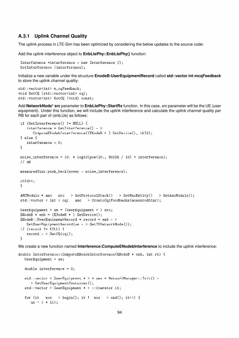
A.3.1 Uplink Channel Quality
The uplink process in LTE-Sim has been optimized by considering the below updates to the source code:
Add the uplink interference object to EnbLtePhy::EnbLtePhy() function:
Interference *interference = new Interference ();
SetInterference (interference);
Initialize a new variable under the structure EnodeB:UserEquipmentRecord called std::vector int mcqFeedbackto store the uplink channel quality:
std::vector<int> m_cqFeedback;
void SetCQ (std::vector<int> cq);
std::vector<int> GetCQ (void) const;
Add NetworkNode* src parameter to EnbLtePhy::StartRx function. In this case, src parameter will be the UE (userequipment). Under this function, we will include the uplink interference and calculate the uplink channel quality perRB for each pair of (enb,Ue) as follows:
if (GetInterference() != NULL) {
interference = GetInterference() - >
ComputeENodebInterference((ENodeB * ) GetDevice(), chId);
} else {
interference = 0;
}
noise_interference = 10. * log10(pow(10., NOISE / 10) + interference);
// dB
measuredSinr.push_back(power - noise_interference);
chId++;
}
AMCModule * amc = src - > GetProtocolStack() - > GetMacEntity() - > GetAmcModule();
std::vector < int > cqi = amc - > CreateCqiFeedbacks(measuredSinr);
UserEquipment * ue = (UserEquipment * ) src;
ENodeB * enb = (ENodeB * ) GetDevice();
ENodeB::UserEquipmentRecord * record = enb - >
GetUserEquipmentRecord(ue - > GetIDNetworkNode());
if (record != NULL) {
record - > SetCQ(cqi);
}
We create a new function named Interference:ComputeENodebInterference to include the uplink interference:
double Interference::ComputeENodebInterference(ENodeB * enb, int rb) {
UserEquipment * ue;
double interference = 0;
std::vector < UserEquipment * > * ues = NetworkManager::Init() -
> GetUserEquipmentContainer();
std::vector < UserEquipment * > ::iterator it;
for (it = ues - > begin(); it != ues - > end(); it++) {
ue = ( * it);
94
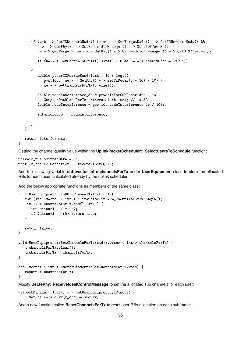
if (enb - > GetIDNetworkNode() != ue - > GetTargetNode() - > GetIDNetworkNode() &&
enb - > GetPhy() - > GetBandwidthManager() - > GetUlOffsetBw() ==
ue - > GetTargetNode() - > GetPhy() - > GetBandwidthManager() - > GetUlOffsetBw())
if (ue - > GetChannelsForTx().size() > 0 && ue - > IsRBinChannelTx(rb))
{
double powerTXForSubBandwidth = 10 * log10(
pow(10., (ue - > GetPhy() - > GetTxPower() - 30) / 10) /
ue - > GetChannelsForTx().size());
double nodeInterference_db = powerTXForSubBandwidth - 10 -
ComputePathLossForInterference(enb, ue); // in dB
double nodeInterference = pow(10, nodeInterference_db / 10);
interference += nodeInterference;
}
}
return interference;
}
Getting the channel quality value within the UplinkPacketScheduler:: SelectUsersToSchedule function:
user->m_transmittedData = 0;
user->m_channelContition = record->GetCQ ();
Add the following variable std::vector int mchannelsForTx under UserEquipment class to store the allocatedRBs for each user, calculated already by the uplink scheduler.
Add the below appropriate functions as members of the same class:
bool UserEquipment::IsRBinChannelTx(int rb) {
for (std::vector < int > ::iterator it = m_channelsForTx.begin();
it != m_channelsForTx.end(); it++) {
int channel = ( * it);
if (channel == rb) return true;
}
return false;
}
void UserEquipment::SetChannelsForTx(std::vector < int > channelsForTx) {
m_channelsForTx.clear();
m_channelsForTx = channelsForTx;
}
std::vector < int > UserEquipment::GetChannelsForTx(void) {
return m_channelsForTx;
}
Modify UeLtePhy::ReceiveIdealControlMessage to set the allocated sub channels for each user:
NetworkManager::Init() - > GetUserEquipmentByID(node) -
> SetChannelsForTx(m_channelsForTx);
Add a new function called ResetChannelsForTx to reset user RBs allocation on each subframe:
95
void UserEquipment::ReSetChannelsForTx() {
m_channelsForTx.clear();
}
A.3.2 Dynamic TDD
This will require adding the function FrameManager::GetMicroSubFrameType and updatingFrameManager::ResourceAllocation function, as per the below :
int FrameManager::GetMicroSubFrameType (int nbSubFrame)
{
return TDDConfigurationMicro [GetMicroTDDFrameConfiguration ()][nbSubFrame-1];
}
void FrameManager::ResourceAllocation(void)
{ .....
if (((record - > GetNodeType() == NetworkNode::TYPE_ENODEB) &&
GetSubFrameType(GetNbSubframes()) == 0) ||
((record - > GetNodeType() == NetworkNode::TYPE_MICROENODEB) &&
GetMicroSubFrameType(GetNbSubframes()) == 0)) {
#
ifdef FRAME_MANAGER_DEBUG
std::cout << " FRAME_MANAGER_DEBUG: SubFrameType = "
" SUBFRAME_FOR_DOWNLINK " << std::endl;#
endif
//record->DownlinkResourceBlokAllocation();
Simulator::Init() - > Schedule(0.0, & ENodeB::DownlinkResourceBlokAllocation, record);
} else if (((record - > GetNodeType() == NetworkNode::TYPE_ENODEB) &&
GetSubFrameType(GetNbSubframes()) == 1) ||
((record - > GetNodeType() == NetworkNode::TYPE_MICROENODEB) &&
GetMicroSubFrameType(GetNbSubframes()) == 1)) {
#
ifdef FRAME_MANAGER_DEBUG
std::cout << " FRAME_MANAGER_DEBUG: SubFrameType = "
" SUBFRAME_FOR_UPLINK " << std::endl;#
endif
//record->UplinkResourceBlockAllocation();
Simulator::Init() - > Schedule(0.0, & ENodeB::UplinkResourceBlockAllocation, record);
}
A.3.3 Cross-link Interference
We first introduce the calculation of the UL to DL interference at the mobile user level with theInterference::ComputeInterference function as follows:
double Interference::ComputeInterference(UserEquipment * ue, int rb) {
ENodeB * node;
UserEquipment * ue1;
ENodeB::UserEquipmentRecord * record;
vector < ENodeB::UserEquipmentRecord * > ::iterator iter;
double interference = 0;
std::vector < ENodeB * > * eNBs = NetworkManager::Init() - > GetENodeBContainer();
std::vector < ENodeB * > ::iterator it;
96
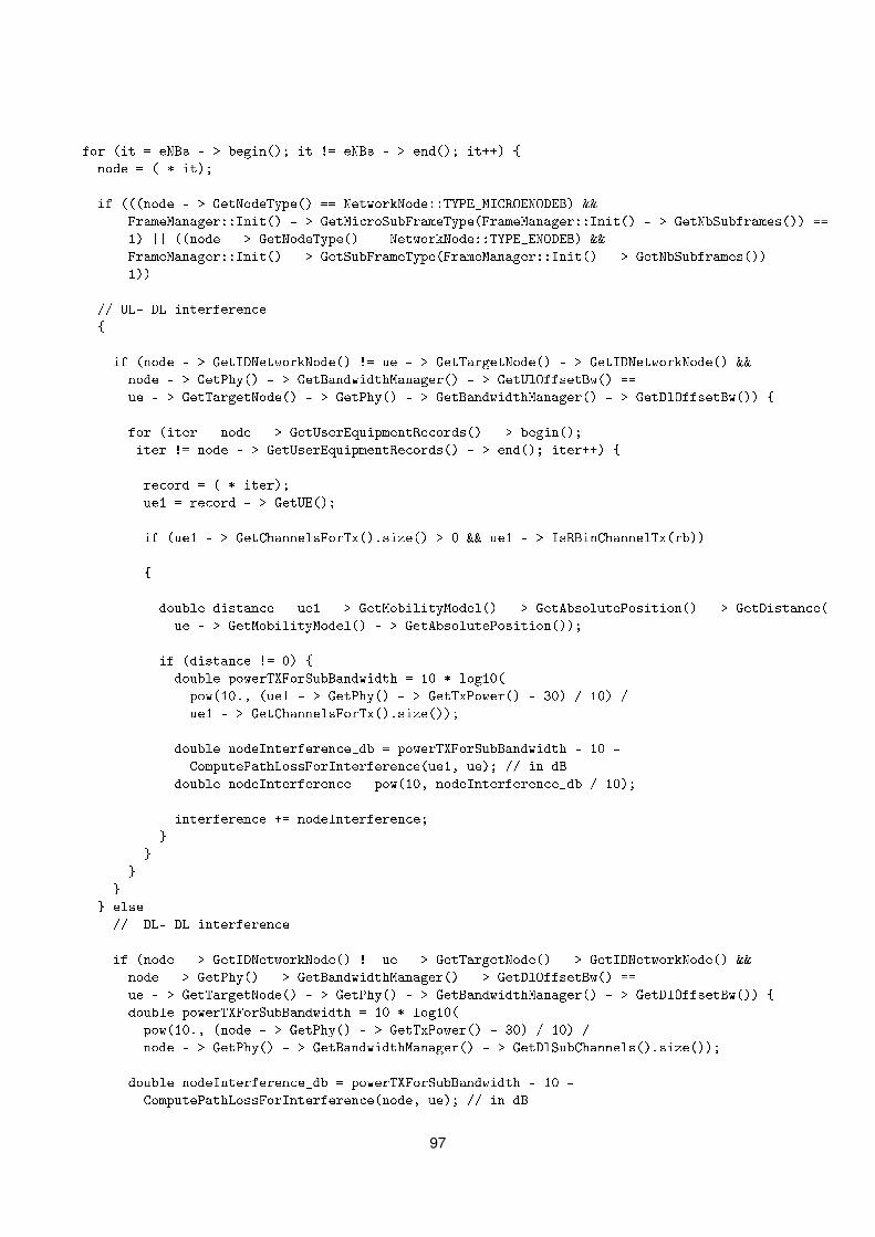
for (it = eNBs - > begin(); it != eNBs - > end(); it++) {
node = ( * it);
if (((node - > GetNodeType() == NetworkNode::TYPE_MICROENODEB) &&
FrameManager::Init() - > GetMicroSubFrameType(FrameManager::Init() - > GetNbSubframes()) ==
1) || ((node - > GetNodeType() == NetworkNode::TYPE_ENODEB) &&
FrameManager::Init() - > GetSubFrameType(FrameManager::Init() - > GetNbSubframes()) ==
1))
// UL- DL interference
{
if (node - > GetIDNetworkNode() != ue - > GetTargetNode() - > GetIDNetworkNode() &&
node - > GetPhy() - > GetBandwidthManager() - > GetUlOffsetBw() ==
ue - > GetTargetNode() - > GetPhy() - > GetBandwidthManager() - > GetDlOffsetBw()) {
for (iter = node - > GetUserEquipmentRecords() - > begin();
iter != node - > GetUserEquipmentRecords() - > end(); iter++) {
record = ( * iter);
ue1 = record - > GetUE();
if (ue1 - > GetChannelsForTx().size() > 0 && ue1 - > IsRBinChannelTx(rb))
{
double distance = ue1 - > GetMobilityModel() - > GetAbsolutePosition() - > GetDistance(
ue - > GetMobilityModel() - > GetAbsolutePosition());
if (distance != 0) {
double powerTXForSubBandwidth = 10 * log10(
pow(10., (ue1 - > GetPhy() - > GetTxPower() - 30) / 10) /
ue1 - > GetChannelsForTx().size());
double nodeInterference_db = powerTXForSubBandwidth - 10 -
ComputePathLossForInterference(ue1, ue); // in dB
double nodeInterference = pow(10, nodeInterference_db / 10);
interference += nodeInterference;
}
}
}
}
} else
// DL- DL interference
if (node - > GetIDNetworkNode() != ue - > GetTargetNode() - > GetIDNetworkNode() &&
node - > GetPhy() - > GetBandwidthManager() - > GetDlOffsetBw() ==
ue - > GetTargetNode() - > GetPhy() - > GetBandwidthManager() - > GetDlOffsetBw()) {
double powerTXForSubBandwidth = 10 * log10(
pow(10., (node - > GetPhy() - > GetTxPower() - 30) / 10) /
node - > GetPhy() - > GetBandwidthManager() - > GetDlSubChannels().size());
double nodeInterference_db = powerTXForSubBandwidth - 10 -
ComputePathLossForInterference(node, ue); // in dB
97
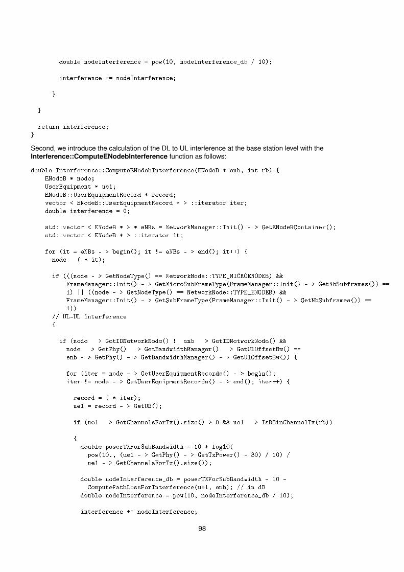
double nodeInterference = pow(10, nodeInterference_db / 10);
interference += nodeInterference;
}
}
return interference;
}
Second, we introduce the calculation of the DL to UL interference at the base station level with theInterference::ComputeENodebInterference function as follows:
double Interference::ComputeENodebInterference(ENodeB * enb, int rb) {
ENodeB * node;
UserEquipment * ue1;
ENodeB::UserEquipmentRecord * record;
vector < ENodeB::UserEquipmentRecord * > ::iterator iter;
double interference = 0;
std::vector < ENodeB * > * eNBs = NetworkManager::Init() - > GetENodeBContainer();
std::vector < ENodeB * > ::iterator it;
for (it = eNBs - > begin(); it != eNBs - > end(); it++) {
node = ( * it);
if (((node - > GetNodeType() == NetworkNode::TYPE_MICROENODEB) &&
FrameManager::Init() - > GetMicroSubFrameType(FrameManager::Init() - > GetNbSubframes()) ==
1) || ((node - > GetNodeType() == NetworkNode::TYPE_ENODEB) &&
FrameManager::Init() - > GetSubFrameType(FrameManager::Init() - > GetNbSubframes()) ==
1))
// UL-UL interference
{
if (node - > GetIDNetworkNode() != enb - > GetIDNetworkNode() &&
node - > GetPhy() - > GetBandwidthManager() - > GetUlOffsetBw() ==
enb - > GetPhy() - > GetBandwidthManager() - > GetUlOffsetBw()) {
for (iter = node - > GetUserEquipmentRecords() - > begin();
iter != node - > GetUserEquipmentRecords() - > end(); iter++) {
record = ( * iter);
ue1 = record - > GetUE();
if (ue1 - > GetChannelsForTx().size() > 0 && ue1 - > IsRBinChannelTx(rb))
{
double powerTXForSubBandwidth = 10 * log10(
pow(10., (ue1 - > GetPhy() - > GetTxPower() - 30) / 10) /
ue1 - > GetChannelsForTx().size());
double nodeInterference_db = powerTXForSubBandwidth - 10 -
ComputePathLossForInterference(ue1, enb); // in dB
double nodeInterference = pow(10, nodeInterference_db / 10);
interference += nodeInterference;
98
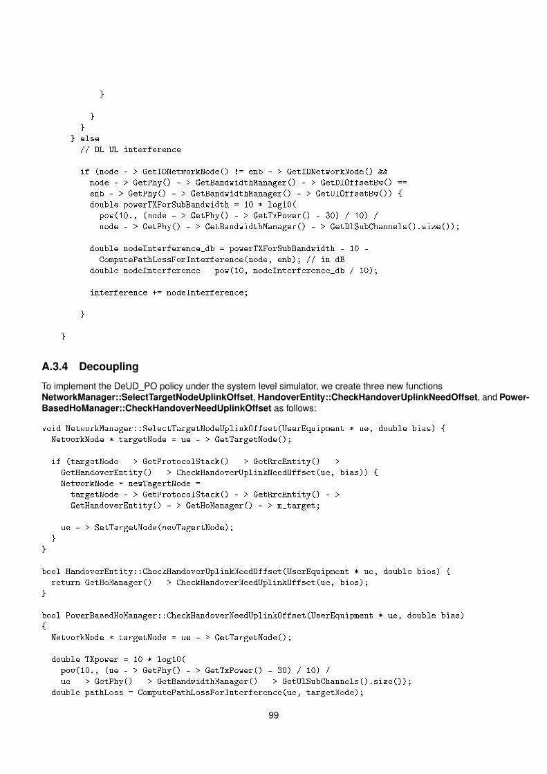
}
}
}
} else
// DL-UL interference
if (node - > GetIDNetworkNode() != enb - > GetIDNetworkNode() &&
node - > GetPhy() - > GetBandwidthManager() - > GetDlOffsetBw() ==
enb - > GetPhy() - > GetBandwidthManager() - > GetUlOffsetBw()) {
double powerTXForSubBandwidth = 10 * log10(
pow(10., (node - > GetPhy() - > GetTxPower() - 30) / 10) /
node - > GetPhy() - > GetBandwidthManager() - > GetDlSubChannels().size());
double nodeInterference_db = powerTXForSubBandwidth - 10 -
ComputePathLossForInterference(node, enb); // in dB
double nodeInterference = pow(10, nodeInterference_db / 10);
interference += nodeInterference;
}
}
A.3.4 Decoupling
To implement the DeUD_PO policy under the system level simulator, we create three new functionsNetworkManager::SelectTargetNodeUplinkOffset, HandoverEntity::CheckHandoverUplinkNeedOffset, and Power-BasedHoManager::CheckHandoverNeedUplinkOffset as follows:
void NetworkManager::SelectTargetNodeUplinkOffset(UserEquipment * ue, double bias) {
NetworkNode * targetNode = ue - > GetTargetNode();
if (targetNode - > GetProtocolStack() - > GetRrcEntity() - >
GetHandoverEntity() - > CheckHandoverUplinkNeedOffset(ue, bias)) {
NetworkNode * newTagertNode =
targetNode - > GetProtocolStack() - > GetRrcEntity() - >
GetHandoverEntity() - > GetHoManager() - > m_target;
ue - > SetTargetNode(newTagertNode);
}
}
bool HandoverEntity::CheckHandoverUplinkNeedOffset(UserEquipment * ue, double bios) {
return GetHoManager() - > CheckHandoverNeedUplinkOffset(ue, bios);
}
bool PowerBasedHoManager::CheckHandoverNeedUplinkOffset(UserEquipment * ue, double bias)
{
NetworkNode * targetNode = ue - > GetTargetNode();
double TXpower = 10 * log10(
pow(10., (ue - > GetPhy() - > GetTxPower() - 30) / 10) /
ue - > GetPhy() - > GetBandwidthManager() - > GetUlSubChannels().size());
double pathLoss = ComputePathLossForInterference(ue, targetNode);
99
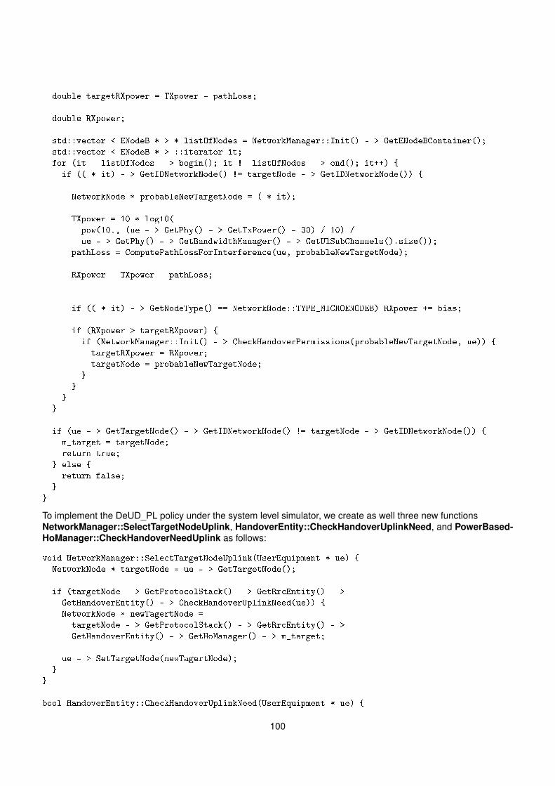
double targetRXpower = TXpower - pathLoss;
double RXpower;
std::vector < ENodeB * > * listOfNodes = NetworkManager::Init() - > GetENodeBContainer();
std::vector < ENodeB * > ::iterator it;
for (it = listOfNodes - > begin(); it != listOfNodes - > end(); it++) {
if (( * it) - > GetIDNetworkNode() != targetNode - > GetIDNetworkNode()) {
NetworkNode * probableNewTargetNode = ( * it);
TXpower = 10 * log10(
pow(10., (ue - > GetPhy() - > GetTxPower() - 30) / 10) /
ue - > GetPhy() - > GetBandwidthManager() - > GetUlSubChannels().size());
pathLoss = ComputePathLossForInterference(ue, probableNewTargetNode);
RXpower = TXpower - pathLoss;
if (( * it) - > GetNodeType() == NetworkNode::TYPE_MICROENODEB) RXpower += bias;
if (RXpower > targetRXpower) {
if (NetworkManager::Init() - > CheckHandoverPermissions(probableNewTargetNode, ue)) {
targetRXpower = RXpower;
targetNode = probableNewTargetNode;
}
}
}
}
if (ue - > GetTargetNode() - > GetIDNetworkNode() != targetNode - > GetIDNetworkNode()) {
m_target = targetNode;
return true;
} else {
return false;
}
}
To implement the DeUD_PL policy under the system level simulator, we create as well three new functionsNetworkManager::SelectTargetNodeUplink, HandoverEntity::CheckHandoverUplinkNeed, and PowerBased-HoManager::CheckHandoverNeedUplink as follows:
void NetworkManager::SelectTargetNodeUplink(UserEquipment * ue) {
NetworkNode * targetNode = ue - > GetTargetNode();
if (targetNode - > GetProtocolStack() - > GetRrcEntity() - >
GetHandoverEntity() - > CheckHandoverUplinkNeed(ue)) {
NetworkNode * newTagertNode =
targetNode - > GetProtocolStack() - > GetRrcEntity() - >
GetHandoverEntity() - > GetHoManager() - > m_target;
ue - > SetTargetNode(newTagertNode);
}
}
bool HandoverEntity::CheckHandoverUplinkNeed(UserEquipment * ue) {
100
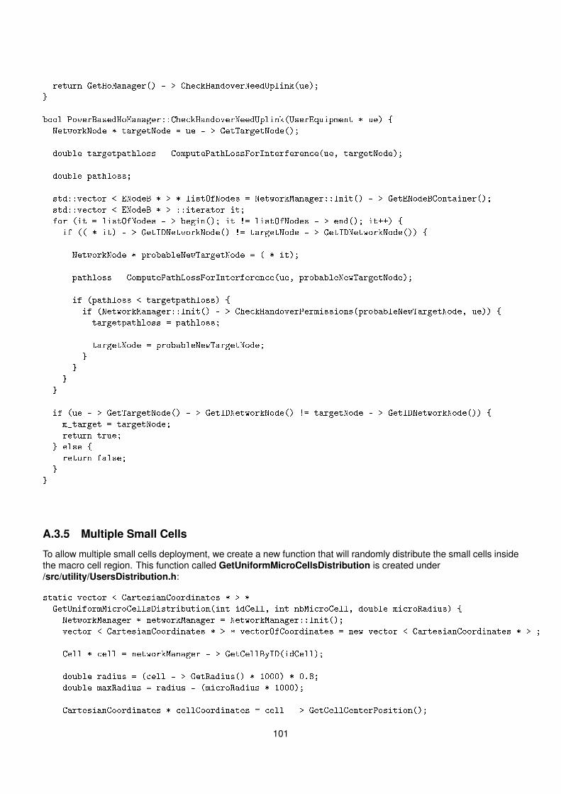
return GetHoManager() - > CheckHandoverNeedUplink(ue);
}
bool PowerBasedHoManager::CheckHandoverNeedUplink(UserEquipment * ue) {
NetworkNode * targetNode = ue - > GetTargetNode();
double targetpathloss = ComputePathLossForInterference(ue, targetNode);
double pathloss;
std::vector < ENodeB * > * listOfNodes = NetworkManager::Init() - > GetENodeBContainer();
std::vector < ENodeB * > ::iterator it;
for (it = listOfNodes - > begin(); it != listOfNodes - > end(); it++) {
if (( * it) - > GetIDNetworkNode() != targetNode - > GetIDNetworkNode()) {
NetworkNode * probableNewTargetNode = ( * it);
pathloss = ComputePathLossForInterference(ue, probableNewTargetNode);
if (pathloss < targetpathloss) {
if (NetworkManager::Init() - > CheckHandoverPermissions(probableNewTargetNode, ue)) {
targetpathloss = pathloss;
targetNode = probableNewTargetNode;
}
}
}
}
if (ue - > GetTargetNode() - > GetIDNetworkNode() != targetNode - > GetIDNetworkNode()) {
m_target = targetNode;
return true;
} else {
return false;
}
}
A.3.5 Multiple Small Cells
To allow multiple small cells deployment, we create a new function that will randomly distribute the small cells insidethe macro cell region. This function called GetUniformMicroCellsDistribution is created under/src/utility/UsersDistribution.h:
static vector < CartesianCoordinates * > *
GetUniformMicroCellsDistribution(int idCell, int nbMicroCell, double microRadius) {
NetworkManager * networkManager = NetworkManager::Init();
vector < CartesianCoordinates * > * vectorOfCoordinates = new vector < CartesianCoordinates * > ;
Cell * cell = networkManager - > GetCellByID(idCell);
double radius = (cell - > GetRadius() * 1000) * 0.8;
double maxRadius = radius - (microRadius * 1000);
CartesianCoordinates * cellCoordinates = cell - > GetCellCenterPosition();
101
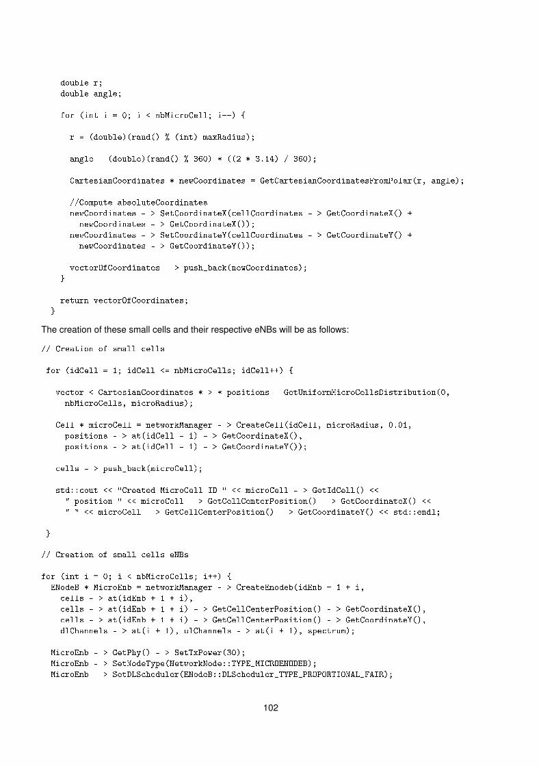
double r;
double angle;
for (int i = 0; i < nbMicroCell; i++) {
r = (double)(rand() % (int) maxRadius);
angle = (double)(rand() % 360) * ((2 * 3.14) / 360);
CartesianCoordinates * newCoordinates = GetCartesianCoordinatesFromPolar(r, angle);
//Compute absoluteCoordinates
newCoordinates - > SetCoordinateX(cellCoordinates - > GetCoordinateX() +
newCoordinates - > GetCoordinateX());
newCoordinates - > SetCoordinateY(cellCoordinates - > GetCoordinateY() +
newCoordinates - > GetCoordinateY());
vectorOfCoordinates - > push_back(newCoordinates);
}
return vectorOfCoordinates;
}
The creation of these small cells and their respective eNBs will be as follows:
// Creation of small cells
for (idCell = 1; idCell <= nbMicroCells; idCell++) {
vector < CartesianCoordinates * > * positions = GetUniformMicroCellsDistribution(0,
nbMicroCells, microRadius);
Cell * microCell = networkManager - > CreateCell(idCell, microRadius, 0.01,
positions - > at(idCell - 1) - > GetCoordinateX(),
positions - > at(idCell - 1) - > GetCoordinateY());
cells - > push_back(microCell);
std::cout << "Created MicroCell ID " << microCell - > GetIdCell() <<
" position " << microCell - > GetCellCenterPosition() - > GetCoordinateX() <<
" " << microCell - > GetCellCenterPosition() - > GetCoordinateY() << std::endl;
}
// Creation of small cells eNBs
for (int i = 0; i < nbMicroCells; i++) {
ENodeB * MicroEnb = networkManager - > CreateEnodeb(idEnb + 1 + i,
cells - > at(idEnb + 1 + i),
cells - > at(idEnb + 1 + i) - > GetCellCenterPosition() - > GetCoordinateX(),
cells - > at(idEnb + 1 + i) - > GetCellCenterPosition() - > GetCoordinateY(),
dlChannels - > at(i + 1), ulChannels - > at(i + 1), spectrum);
MicroEnb - > GetPhy() - > SetTxPower(30);
MicroEnb - > SetNodeType(NetworkNode::TYPE_MICROENODEB);
MicroEnb - > SetDLScheduler(ENodeB::DLScheduler_TYPE_PROPORTIONAL_FAIR);
102
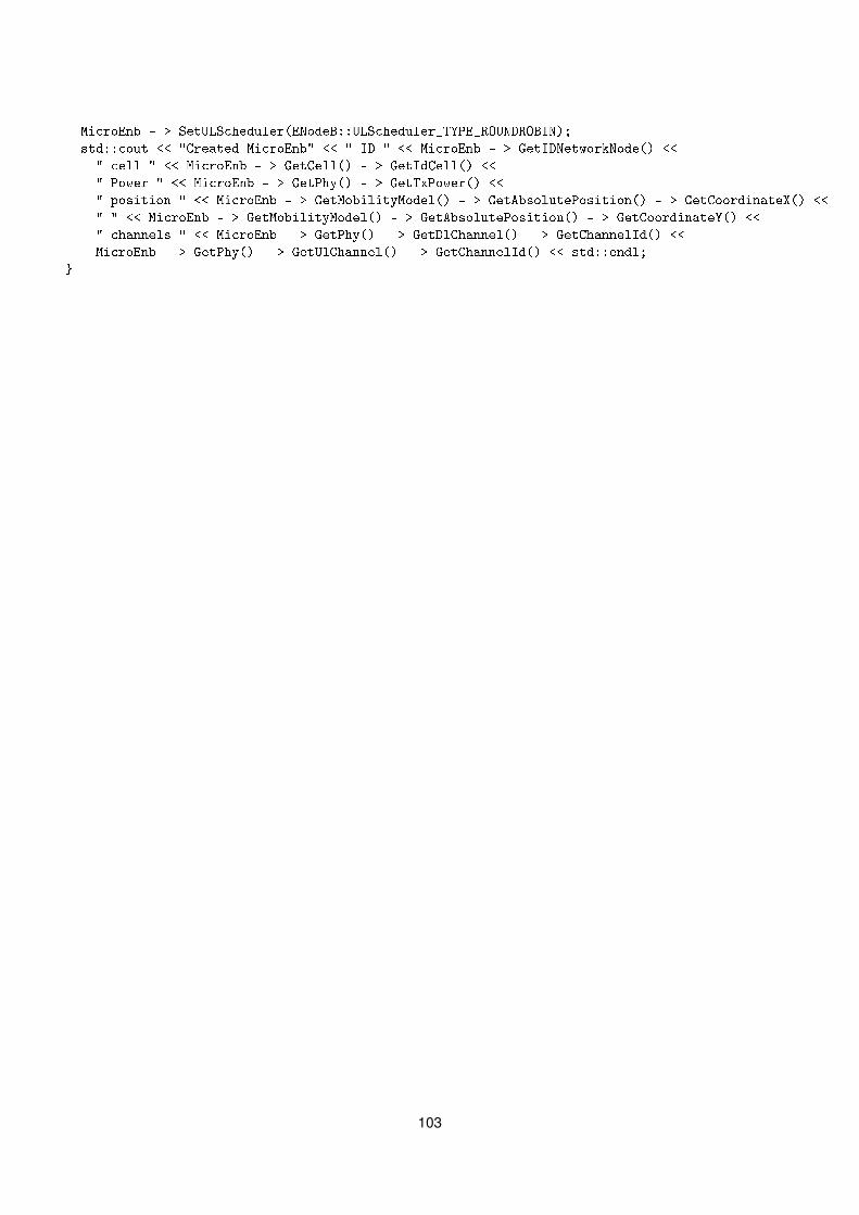
MicroEnb - > SetULScheduler(ENodeB::ULScheduler_TYPE_ROUNDROBIN);
std::cout << "Created MicroEnb" << " ID " << MicroEnb - > GetIDNetworkNode() <<
" cell " << MicroEnb - > GetCell() - > GetIdCell() <<
" Power " << MicroEnb - > GetPhy() - > GetTxPower() <<
" position " << MicroEnb - > GetMobilityModel() - > GetAbsolutePosition() - > GetCoordinateX() <<
" " << MicroEnb - > GetMobilityModel() - > GetAbsolutePosition() - > GetCoordinateY() <<
" channels " << MicroEnb - > GetPhy() - > GetDlChannel() - > GetChannelId() <<
MicroEnb - > GetPhy() - > GetUlChannel() - > GetChannelId() << std::endl;
}
103

Publications
Conferences
[128] B. Lahad, M. Ibrahim, S. Lahoud, K. Khawam and S. Martin,“A Statistical Model for Uplink/Downlink IntercellInterference and Cell Capacity in TDD HetNets," 2018 IEEE International Conference on Communications(ICC), Kansas City, MO, USA, 2018, pp. 1-6
[129] B. Lahad, M. Ibrahim, S. Lahoud, K. Khawam and S. Martin,“Analytical Evaluation of Decoupled Uplink andDownlink Access in TDD 5G HetNets," 2018 IEEE 29th Annual International Symposium on Personal, Indoorand Mobile Radio Communications (PIMRC), Bologna, Italy, 2018, pp. 1-7.
[131] B. Lahad, M. Ibrahim, S. Lahoud, K. Khawam and S. Martin,“Uplink/Downlink Decoupled Access with DynamicTDD in 5G HetNets," 2020 IEEE International conference on Wireless Communications and Mobile Computing(IWCMC), Limassol, Cyprus, 2020, pp. 1-6.
Journal in IEEE Transactions on Mobile Computing
[130] B. Lahad, M. Ibrahim, S. Lahoud, K. Khawam and S. Martin,“Joint Modeling of TDD and Decoupled Up-link/Downlink Access in 5G HetNets with Multiple Small Cells Deployment," Accepted in IEEE Transactions onMobile Computing, 2020.
105

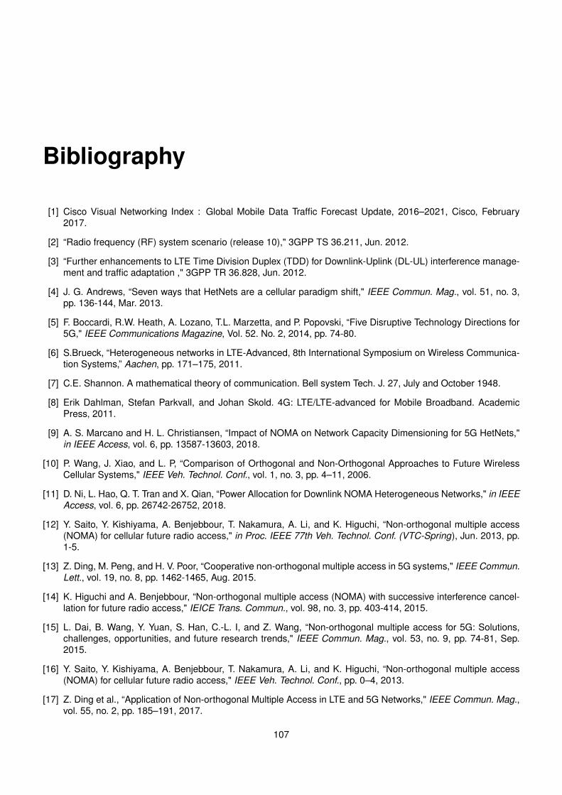
Bibliography
[1] Cisco Visual Networking Index : Global Mobile Data Traffic Forecast Update, 2016–2021, Cisco, February2017.
[2] “Radio frequency (RF) system scenario (release 10)," 3GPP TS 36.211, Jun. 2012.
[3] “Further enhancements to LTE Time Division Duplex (TDD) for Downlink-Uplink (DL-UL) interference manage-ment and traffic adaptation ," 3GPP TR 36.828, Jun. 2012.
[4] J. G. Andrews, “Seven ways that HetNets are a cellular paradigm shift," IEEE Commun. Mag., vol. 51, no. 3,pp. 136-144, Mar. 2013.
[5] F. Boccardi, R.W. Heath, A. Lozano, T.L. Marzetta, and P. Popovski, “Five Disruptive Technology Directions for5G," IEEE Communications Magazine, Vol. 52. No. 2, 2014, pp. 74-80.
[6] S.Brueck, “Heterogeneous networks in LTE-Advanced, 8th International Symposium on Wireless Communica-tion Systems,” Aachen, pp. 171–175, 2011.
[7] C.E. Shannon. A mathematical theory of communication. Bell system Tech. J. 27, July and October 1948.
[8] Erik Dahlman, Stefan Parkvall, and Johan Skold. 4G: LTE/LTE-advanced for Mobile Broadband. AcademicPress, 2011.
[9] A. S. Marcano and H. L. Christiansen, “Impact of NOMA on Network Capacity Dimensioning for 5G HetNets,"in IEEE Access, vol. 6, pp. 13587-13603, 2018.
[10] P. Wang, J. Xiao, and L. P, “Comparison of Orthogonal and Non-Orthogonal Approaches to Future WirelessCellular Systems," IEEE Veh. Technol. Conf., vol. 1, no. 3, pp. 4–11, 2006.
[11] D. Ni, L. Hao, Q. T. Tran and X. Qian, “Power Allocation for Downlink NOMA Heterogeneous Networks," in IEEEAccess, vol. 6, pp. 26742-26752, 2018.
[12] Y. Saito, Y. Kishiyama, A. Benjebbour, T. Nakamura, A. Li, and K. Higuchi, “Non-orthogonal multiple access(NOMA) for cellular future radio access," in Proc. IEEE 77th Veh. Technol. Conf. (VTC-Spring), Jun. 2013, pp.1-5.
[13] Z. Ding, M. Peng, and H. V. Poor, “Cooperative non-orthogonal multiple access in 5G systems," IEEE Commun.Lett., vol. 19, no. 8, pp. 1462-1465, Aug. 2015.
[14] K. Higuchi and A. Benjebbour, “Non-orthogonal multiple access (NOMA) with successive interference cancel-lation for future radio access," IEICE Trans. Commun., vol. 98, no. 3, pp. 403-414, 2015.
[15] L. Dai, B. Wang, Y. Yuan, S. Han, C.-L. I, and Z. Wang, “Non-orthogonal multiple access for 5G: Solutions,challenges, opportunities, and future research trends," IEEE Commun. Mag., vol. 53, no. 9, pp. 74-81, Sep.2015.
[16] Y. Saito, Y. Kishiyama, A. Benjebbour, T. Nakamura, A. Li, and K. Higuchi, “Non-orthogonal multiple access(NOMA) for cellular future radio access," IEEE Veh. Technol. Conf., pp. 0–4, 2013.
[17] Z. Ding et al., “Application of Non-orthogonal Multiple Access in LTE and 5G Networks," IEEE Commun. Mag.,vol. 55, no. 2, pp. 185–191, 2017.
107
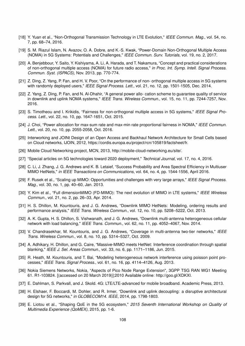
[18] Y. Yuan et al., “Non-Orthogonal Transmission Technology in LTE Evolution," IEEE Commun. Mag., vol. 54, no.7, pp. 68–74, 2016.
[19] S. M. Riazul Islam, N. Avazov, O. A. Dobre, and K.-S. Kwak, “Power-Domain Non-Orthogonal Multiple Access(NOMA) in 5G Systems: Potentials and Challenges," IEEE Commun. Surv. Tutorials, vol. 19, no. 2, 2017.
[20] A. Benjebbour, Y. Saito, Y. Kishiyama, A. Li, A. Harada, and T. Nakamura, “Concept and practical considerationsof non-orthogonal multiple access (NOMA) for future radio access," in Proc. Int. Symp. Intell. Signal Process.Commun. Syst. (ISPACS), Nov. 2013, pp. 770-774.
[21] Z. Ding, Z. Yang, P. Fan, and H. V. Poor, “On the performance of non- orthogonal multiple access in 5G systemswith randomly deployed users," IEEE Signal Process. Lett., vol. 21, no. 12, pp. 1501-1505, Dec. 2014.
[22] Z. Yang, Z. Ding, P. Fan, and N. Al-Dhahir, “A general power allo- cation scheme to guarantee quality of servicein downlink and uplink NOMA systems," IEEE Trans. Wireless Commun., vol. 15, no. 11, pp. 7244-7257, Nov.2016.
[23] S. Timotheou and I. Krikidis, “Fairness for non-orthogonal multiple access in 5G systems," IEEE Signal Pro-cess. Lett., vol. 22, no. 10, pp. 1647-1651, Oct. 2015.
[24] J. Choi, “Power allocation for max-sum rate and max-min rate proportional fairness in NOMA," IEEE Commun.Lett., vol. 20, no. 10, pp. 2055-2058, Oct. 2016.
[25] Interworking and JOINt Design of an Open Access and Backhaul Network Architecture for Small Cells basedon Cloud networks, IJOIN, 2012, https://cordis.europa.eu/project/rcn/105819/factsheet/fr.
[26] Mobile Cloud Networking project, MCN, 2013, http://mobile-cloud-networking.eu/site/.
[27] “Special articles on 5G technologies toward 2020 deployment," Technical Journal, vol. 17, no. 4, 2016.
[28] C. Li, J. Zhang, J. G. Andrews and K. B. Letaief, “Success Probability and Area Spectral Efficiency in MultiuserMIMO HetNets," in IEEE Transactions on Communications, vol. 64, no. 4, pp. 1544-1556, April 2016.
[29] F. Rusek et al., “Scaling up MIMO: Opportunities and challenges with very large arrays," IEEE Signal Process.Mag., vol. 30, no. 1, pp. 40–60, Jan. 2013.
[30] Y. Kim et al., “Full dimensionMIMO (FD-MIMO): The next evolution of MIMO in LTE systems," IEEE WirelessCommun., vol. 21, no. 2, pp. 26–33, Apr. 2014.
[31] H. S. Dhillon, M. Kountouris, and J. G. Andrews, “Downlink MIMO HetNets: Modeling, ordering results andperformance analysis," IEEE Trans. Wireless Commun., vol. 12, no. 10, pp. 5208–5222, Oct. 2013.
[32] A. K. Gupta, H. S. Dhillon, S. Vishwanath, and J. G. Andrews, “Downlink multi-antenna heterogeneous cellularnetwork with load balancing," IEEE Trans. Commun., vol. 62, no. 11, pp. 4052–4067, Nov. 2014.
[33] V. Chandrasekhar, M. Kountouris, and J. G. Andrews, “Coverage in multi-antenna two-tier networks," IEEETrans. Wireless Commun., vol. 8, no. 10, pp. 5314–5327, Oct. 2009.
[34] A. Adhikary, H. Dhillon, and G. Caire, “Massive-MIMO meets HetNet: Interference coordination through spatialblanking," IEEE J. Sel. Areas Commun., vol. 33, no. 6, pp. 1171–1186, Jun. 2015.
[35] R. Heath, M. Kountouris, and T. Bai, “Modeling heterogeneous network interference using poisson point pro-cesses," IEEE Trans. Signal Process., vol. 61, no. 16, pp. 4114–4126, Aug. 2013.
[36] Nokia Siemens Networks, Nokia, “Aspects of Pico Node Range Extension", 3GPP TSG RAN WG1 Meeting61. R1-103824. [(accessed on 20 March 2019)];2010 Available online: http://goo.gl/XDKXI.
[37] E. Dahlman, S. Parkvall, and J. Skold. 4G: LTE/LTE-advanced for mobile broadband. Academic Press, 2013.
[38] H. Elshaer, F. Boccardi, M. Dohler, and R. Irmer, “Downlink and uplink decoupling: a disruptive architecturaldesign for 5G networks," in GLOBECOM14. IEEE, 2014, pp. 1798-1803.
[39] E. Liotou et al., “Shaping QoE in the 5G ecosystem," 2015 Seventh International Workshop on Quality ofMultimedia Experience (QoMEX), 2015, pp. 1-6.
108
[40] 3GPP TR 36.819, “Coordinated multi-point operation for LTE physical layer aspects," V.11.1.0, December 2011.
[41] A. He, D. Liu, Y. Chen and T. Zhang, “Stochastic geometry analysis of energy efficiency in HetNets with com-bined CoMP and BS sleeping," 2014 IEEE 25th Annual International Symposium on Personal, Indoor, andMobile Radio Communication (PIMRC), Washington, DC, 2014, pp. 1798-1802.
[42] Tao Han and N. Ansari. On greening cellular networks via multicell cooperation. IEEE Commun. Mag.,20(1):82–89, 2013.
[43] G. Cili, H. Yanikomeroglu, and F.R. Yu. Cell switch off technique combined with coordinated multi-point (comp)transmission for energy efficiency in beyond-lte cellular networks. In IEEE Int. Conf. Commun. (ICC), pages5931–5935. IEEE, 2012.
[44] H. ElSawy, E. Hossain, and M. Haenggi. Stochastic geometry for modeling, analysis, and design of multi-tierand cognitive cellular wireless networks: A survey. IEEE Commun. Surveys & Tutorials, 15(3):996–1019, 2013.
[45] J.G. Andrews, F. Baccelli, and R.K. Ganti. A tractable approach to coverage and rate in cellular networks. IEEETrans. Commun., 59(11):3122–3134, 2011.
[46] H.S. Dhillon, R.K. Ganti, F. Baccelli, and J.G. Andrews. Modeling and analysis of k-tier downlink heterogeneouscellular networks. IEEE J. Sel. Areas Commun, 30(3):550–560, 2012.
[47] K. M. S. Huq, S. Mumtaz, J. Bachmatiuk, J. Rodriguez, X. Wang and R. L. Aguiar, “Green HetNet CoMP:Energy Efficiency Analysis and Optimization," in IEEE Transactions on Vehicular Technology, vol. 64, no. 10,pp. 4670-4683, Oct. 201
[48] 3GPP. Coordinated Multi-Point Operation for LTE Physical Layer Aspects. TS 36.819, 3rd Generation Partner-ship Project (3GPP), September 2012.
[49] 3GPP. LTE Radio Access Network (RAN) Enhancements for Diverse Data Applications. TR 36.822, 3rd Gen-eration Partnership Project (3GPP), September 2012.
[50] 3GPP. Technical Specification Group Radio Access Network; Evolved Universal Terrestrial Radio Access (E-UTRA) and Evolved Universal Terrestrial Radio Access Network (E-UTRAN); Overall description; Stage 2(Release 11). TS 36.300, 3rd Generation Partnership Project (3GPP), September 2012.
[51] 3GPP. Study on Small Cell Enhancements for E-UTRA and E-UTRAN; Higher Layer Aspects. TR 36.842, 3rdGeneration Partnership Project (3GPP), September 2014.
[52] F. Boccardi, J. Andrews, H. Elshaer, M. Dohler, S. Parkvall, P. Popovski, and S. Singh, “Why to decouple theuplink and downlink in cellular networks and how to do it," arXiv preprint arXiv:1503.06746, 2015.
[53] H. A. Mustafa, M. Z. Shakir, Y. A. Sambo, K. A. Qaraqe, M. A. Imran and E. Serpedin,“Spectral efficiencyimprovements in HetNets by exploiting device-to-device communications," 2014 IEEE Globecom Workshops(GC Wkshps), Austin, TX, 2014, pp. 857-862
[54] Astely, D., Dahlman, E., Fodor, G., Parkvall, S. and Sachs, J. (2013) LTE Release 12 and Beyond Acceptedfrom Open Call. IEEE Communications Magazine, 51, 154-160. https://doi.org/10.1109/MCOM.2013.6553692
[55] K. Doppler, M. Rinne, C. Wijting, C. Ribeiro, and K. Hugl, “Device-to-device communication as an underlay toLTE-advanced networks," in IEEE Mag. Communs., vol. 27, no. 12, pp. 42–49, Dec. 2009.
[56] P. Janis, C.-H. Yu, K. Doppler, C. B. Ribeiro, C. Wijting, K. Hugl, O. Tirkkonen, and V. Koivunen,“Device-todevice communication underlying cellular communications systems," in Intl. Jour. Commun., Network andSystem Sciences, vol. 2, no. 3, pp. 169–178, 2009.
[57] S. Hakola, T. Chen, J. Lehtomäki, and T. Koskela, “Device-to-device (D2D) communication in cellular network -performance analysis of optimum and practical communication mode selection," pp. 1–6, Apr. 2010.
[58] Lin, X., Andrews, J.G., Ghosh, A. and Ratasuk, R. (2014) An Overview of 3GPP Device-to-Device ProximityServices. IEEE Communications Magazine, 52, 40-48. https://doi.org/10.1109/MCOM.2014.6807945
109
[59] Omran, A., BenMimoune, A. and Kadoch, M. (2017) Mobility Management for D4D in HetNet. 2017 IEEE 30thCanadian Conference on Electrical and Computer Engineering, Windsor, Canada, 30 April-3 May 2017, 1-5.https://doi.org/10.1109/CCECE.2017.7946632
[60] Huq, K.M.S., Mumtaz, S., Rodriguez, J., Marques, P., Okyere, B. and Frascolla, V. (2017)Enhanced C-RAN Using D2D Network. IEEE Communications Magazine, 55, 100-107.https://doi.org/10.1109/MCOM.2017.1600497CM
[61] S. Guo, X. Hou and H. Wang, “Dynamic TDD and interference management towards 5G,"2018 IEEE WirelessCommunications and Networking Conference (WCNC), 2018, pp. 1-6.
[62] “Radio frequency (RF) system scenario (release 10)," 3GPP TS 36.211, Jun. 2012.
[63] 3GPP, TR36.828 (v11.4.0), “Further enhancements to LTE TDD for DL-UL interference management and trafficadaptation”, Jun. 2012.
[64] S. Sesia, I. Touk, and M. Baker, LTE - The UMTS Long Term Evolution: From Theory to Practice, John Wiley &Sons, Ltd, 2009.
[65] K. Smiljkovikj, H. Elshaer, P. Popovski, F. Boccardi, M. Dohler, L. Gavrilovska, and R. Irmer, “Capacity analysisof decoupled down- link and uplink access in 5G heterogeneous systems," arXiv preprint arXiv:1410.7270,2014.
[66] X. Liu, R. Li, K. Luo, and T. Jiang, “Downlink and uplink decoupling in heterogeneous networks for 5G andbeyond," J. Commun. Inf. Netw., vol. 3, no. 2, pp. 1–13, 2018.
[67] N. H. M. Adnan, I. M. Rafiqul and A. H. M. Z. Alam, “Massive MIMO for Fifth Generation (5G): Opportunities andChallenges," 2016 International Conference on Computer and Communication Engineering (ICCCE), 2016, pp.47-52.
[68] C. Seker, M. T. Güneser and T. Ozturk, “A Review of Millimeter Wave Communication for 5G," 2018 2ndInternational Symposium on Multidisciplinary Studies and Innovative Technologies (ISMSIT), 2018, pp. 1-5.
[69] Huawei has showcased its ability to improve 5G coverage, capacity, and user experience by carryinguplink data via 4G LTE bands and downlink data on 5G bands, 2017 Nov [accessed 2021 Aug 26].https://www.zdnet.com/article/huawei-demos-5g-uplink-downlink-decoupling-tech/.
[70] Huawei ’s “5G UL & DL Decoupling" Receives 2019 GSMA Award for Best Mobile Technology Breakthrough,2019 Feb [accessed 2021 Aug 26]. https://www.huawei.com/en/press-events/news/2019/2/huawei-5g-ul-dl-decoupling-awarded.
[71] “NR; User Equipment (UE) radio transmission and reception; Part 3: Range 1 and Range 2 Interworkingoperation with other radios (release 16)," 3GPP TS 38.101-3, Jan. 2020.
[72] “NR; User Equipment (UE) radio transmission and reception; Part 2: Range 2 Standalone (release 16)," 3GPPTS 38.101-2, Jan. 2020.
[73] “NR; User Equipment (UE) radio transmission and reception; Part 1: Range 1 Standalone (release 16)," 3GPPTS 38.101-1, Jan. 2020.
[74] Developing mmWave mobile radio interface, 2017 Aug. https://www.ericsson.com/en/blog/2017/8/developing-mmwave-mobile-radio-interface.
[75] K. W. Sung, H. Haas, and S. McLaughlin, “A semi-analytical PDF of downlink SINR for femtocell networks,"EURASIP J. Wireless Commun. and Networking, Jan. 2010.
[76] S. Plass, X. G. Doukopoulos, and R. Legouable, “Investigations on link-level inter-cell interference in OFDMAsystems," in Proc. 2006 IEEE Symposium on Communications and Vehicular Technology, pp. 49-52.
[77] X. Yang and A. O. Fapojuwo, “Analysis of heterogeneous cellular network with hexagonal tessellated macrocellsand randomly positioned small cells," IEEE WCNC, 2016.
110
[78] M. Taranetz and M. Rupp, “A circular interference model for wireless cellular networks," International WirelessCommunications and Mobile Computing Conference, 2014.
[79] C. Seol and K. Cheun, “A Statistical Inter-cell Interference Model for Downlink Cellular OFDMA Networks underLog-normal Shadowing and Multipath Rayleigh Fading," IEEE Transactions on Communications, vol. 57, no.10, pp. 3069–3077, October 2009.
[80] C. Seol, K. Cheun, and S. Hong, “A Statistical Inter-cell Interference Model for Downlink Cellular OFDMANetworks under Log-normal Shadowing with Ricean Fading," IEEE Communications Letters, vol. 14, no. 11,pp. 1011–1013, November 2010.
[81] S. Elayoubi, B. Haddada, and B. Fourestie, “Performance evaluation of frequency planning schemes in OFDMAbased networks," IEEE Trans.Wireless Commun., vol. 7, no. 5, pp. 1623-1633, May 2008.
[82] R. Kwan and C. Leung, “On collision probabilities in frequency-domain scheduling for LTE cellular networks,"IEEE Commun. Lett., vol. 15, no. 9, pp. 965- 967, Sep. 2011.
[83] I. Viering, A. Klein, M. Ivrlac, M. Castaneda, and J. A. Nossek, “On uplink intercell interference in a cellularsystem," in Proc. 2006 IEEE International Conference on Communications, pp. 2095-2100.
[84] M. Ding, D. Lopez-Perez, G. Mao, and Z. Lin, “DNA-GA: A new approach of network performance analysis,"Proc. IEEE ICC 2016,arXiv:1512.05429 [cs.IT], to be published.
[85] H. Tabassum, Z. Dawy, E. Hossain, and M. S Alouini, “A framework for uplink intercell interference modelingwith channel-based scheduling," IEEE Trans. Wireless Commun., vol. 12, no. 1, pp. 206-217, Jan. 2013.
[86] H. Tabassum, Z. Dawy, E. Hossain, and M. S Alouini, “Interference statistics and capacity analysis for uplinktransmission in two-tier small cell networks: A geometric probability approach," IEEE Trans. Wireless Commun.,vol. 13, no. 7, pp. 3837-3852, Jul. 2014.
[87] Ahmad El-Hajj, Naeem Akl, Bilal Hammoud, and Zaher Dawy, “On interference modeling for the analysisof uplink/downlink interactions in TDD-OFDMA networks," 2015 International Wireless Communications andMobile Computing Conference (IWCMC), pp. 497-502, 2015.
[88] F. Boccardi, J. Andrews, H. Elshaer, M. Dohler, S. Parkvall, P. Popovski, and S. Singh, “Why to decouple theuplink and downlink in cellular networks and how to do it," arXiv preprint arXiv:1503.06746, 2015.
[89] H. Elshaer, F. Boccardi, M. Dohler, and R. Irmer, “Downlink and uplink decoupling: a disruptive architecturaldesign for 5G networks," in GLOBECOM’14. IEEE, 2014, pp. 1798-1803.
[90] “Load & backhaul aware decoupled downlink/uplink access in 5G systems," arXiv preprint arXiv:1410.6680,2014.
[91] Qualcomm, “Range expansion for efficient support of heterogeneous networks," 3GPP TSG-RAN WG1 R1-083813, 2008.
[92] K. Smiljkovikj, H. Elshaer, P. Popovski, F. Boccardi, M. Dohler, L. Gavrilovska, and R. Irmer, “Capacity analysisof decoupled down- link and uplink access in 5G heterogeneous systems," arXiv preprint arXiv:1410.7270,2014.
[93] K. Smiljkovikj, P. Popovski, and L. Gavrilovska, “Analysis of the decoupled access for downlink and uplink inwireless heterogeneous networks," Wireless Communications Letters, IEEE, vol. 4, no. 2, pp. 173-176, 2015.
[94] H. ElSawy, E. Hossain, and M. Haenggi, “Stochastic Geometry for Modeling, Analysis, and Design of Multi-Tierand Cognitive Cellular Wireless Networks: A Survey," IEEE Comm. Surveys & Tutorials, Vol.15, No. 3, 2013
[95] W. Nie, L. Zhang, and G. Fang, “Uplink Performance Improvement by Decoupling Uplink/Downlink Access inHetNets," IEEE Transactions on Vehicular Technology, IEEE, vol. 66, no. 8, pp. 6862-6876, 2017.
[96] H. E. Shaer, M. N. Kulkarni, F. Boccardi, J. G. Andrews, and M. Dohler, “Downlink and Uplink Cell Associationin Sub-6GHz and Millimeter Wave 5G Heterogeneous Networks," Globecom Workshops (GC Wkshps), 2016IEEE.
111
[97] Ahmad El-Hajj, Naeem Akl, Bilal Hammoud, and Zaher Dawy, “On interference modeling for the analysisof uplink/downlink interactions in TDD-OFDMA networks," 2015 International Wireless Communications andMobile Computing Conference (IWCMC), pp. 497-502, 2015.
[98] H. Mehrpouyan, M. Matthaiou, R. Wang, G. K. Karagiannidis, and Y. Hua, “Hybrid millimeter-wave systems: Anovel paradigm for HetNets," IEEE Commun. Mag., vol. 53, no. 1, pp. 216-221, Jan. 2015.
[99] H. Elshaer, F. Boccardi, M. Dohler, and R. Irmer, “Downlink and uplink decoupling: a disruptive architecturaldesign for 5G networks," in GLOBECOM’14. IEEE, 2014, pp. 1798-1803.
[100] “Load & backhaul aware decoupled downlink/uplink access in 5G systems," arXiv preprint arXiv:1410.6680,2014.
[101] Qualcomm, “Range expansion for efficient support of heterogeneous networks," 3GPP TSG-RAN WG1 R1-083813, 2008.
[102] M. S. ElBamby, M. Bennis, and M. Latva-aho, “UL/DL decoupled user association in dynamic TDD small cellnetworks," in 2015 International Symposium on Wireless Communication Systems (ISWCS), Aug 2015, pp.456–460.
[103] B. Lahad, M. Ibrahim, S. Lahoud, K. Khawam and S. Martin,“A Statistical Model for Uplink/Downlink IntercellInterference and Cell Capacity in TDD HetNets," 2018 IEEE International Conference on Communications(ICC), 2018, pp. 1-6.
[104] Q. Liao, D. Aziz, and S. Stanczak, “Dynamic joint uplink and downlink optimization for uplink anddownlink decoupling-enabled 5G heterogeneous networks," arXiv preprint, 2016. [Online]. Available:http://arxiv.org/abs/1607.05459 13dB
[105] S. Singh, X. Zhang and J. G. Andrews, “Joint Rate and SINR Coverage Analysis for Decoupled Uplink-Downlink Biased Cell Associations in HetNets," in IEEE Transactions on Wireless Communications, vol. 14, no.10, pp. 5360-5373, Oct. 2015.
[106] 3GPP, Tech. Specif. Group Radio Access Networks; Radio Frequency (RF) system scenarios (Release 9),3GPP TS 25.942.
[107] 3GPP, Tech. Specif. Group Radio Access Network; Evolved Universal Terrestrial Radio Access (E-UTRA)and Evolved Universal Terrestrial Radio Access Network (E-UTRAN); Radio Frequency (RF) system scenarios(Release 10), 3GPP TS 36.942.
[108] 3GPP TS 36.213, v11.3.0, “Evolved Universal Terrestrial Radio Access (E-UTRA); Physical layer procedures,"Jun. 2013.
[109] 3GPP TS 36.213, v11.3.0, “Evolved Universal Terrestrial Radio Access (E-UTRA); Physical layer procedures,"Jun. 2013.
[110] Weisstein, Eric W. "Circle-Circle Intersection." From MathWorld–A Wolfram Web Resource.https://mathworld.wolfram.com/Circle-CircleIntersection.html.
[111] “Chain Rule in Leibniz Notation," oregonstate.edu., Retrieved 2019-07-28.
[112] K. A. Hamdi, “A useful lemma for capacity analysis of fading interference channels," IEEE Trans. Commun.,vol. 58, no. 2, pp. 411-416, Feb. 2010.
[113] Mathar, R. (2013). GAUSS-LAGUERRE AND GAUSS-HERMITE QUADRATURE ON 64, 96 AND 128NODES. viXra.
[114] Philip Rabinowitz and George Weiss, Tables of abscissas and weights for numerical evaluation of integrals ofthe form
∫∞0e−xxnf(x)dx, Math. Comp. 13 (1959), 285–294. MR 0107992.
[115] D. Fairthorne, “The distances between random points in two concentric circles," Biometrika, vol. 51, no. 1/2,pp. 275-277, Jun. 1964.
112
[116] Nokia Siemens Networks, Nokia, “Aspects of Pico Node Range Extension", 3GPP TSG RAN WG1 Meeting61. R1-103824. [(accessed on 20 March 2019)];2010 Available online: http://goo.gl/XDKXI.
[117] B. Lahad, M. Ibrahim, S. Lahoud, K. Khawam and S. Martin,“Analytical Evaluation of Decoupled Uplink andDownlink Access in TDD 5G HetNets," 2018 IEEE 29th Annual International Symposium on Personal, Indoorand Mobile Radio Communications (PIMRC), Bologna, Italy, 2018, pp. 1-7.
[118] 3GPP, TR25.951 (v10.0.0), “Technical Specification Group Radio Access Network; Evolved Universal Terres-trial Radio Access (E-UTRA); Radio Frequency (RF) system scenarios (Release 10)”, Dec. 2010.
[119] 3GPP, TR25.951 (v10.0.0), “ Technical Specification Group Radio Access Network; FDD Base Station (BS)classification (Release 10)”, Apr. 2011.
[120] “3GPP TS 136.300, Evolved Universal Terrestrial Radio Access (EUTRA) and Evolved Universal TerrestrialRadio Access Network (EUTRAN); Overall description; Stage 2 (Release 10),” 2011.
[121] G. Piro, L. A. Grieco, G. Boggia, F. Capozzi, and P. Camarda,“Simulating LTE Cellular Systems: An Open-Source Framework,"IEEE Trans. Veh. Technol., vol. 60, no. 2, pp. 498-513, Feb. 2011.
[122] J. W. C, Microwave Mobile Communications New York. Wiley. 1975.
[123] M. Lord and D. Memmi, “NetSim: a Simulation and Visualization Software for Information Network Modeling,"in e-Technologies, International MCETECH Conference, pp. 167-177, 2008.
[124] X. Chang,“Network simulations with OPNET," in Proc. 31st Conf. Winter Simulation: Simulation—A Bridge tothe Future Volume 1, WSC’99, New York, 1999, pp. 307–314.
[125] M. Rupp, S. Schwarz, and M. Taranetz,“The Vienna LTE-Advanced Simulators: Up and Downlink, Link andSystem Level Simulation," Springer, 2016.
[126] G. F. Riley and T. R. Henderson, “The ns-3 Network Simulator," in Modeling and Tools for Network Simulation,Berlin, Heidelberg: Springer Berlin Heidelberg, 2010, pp. 15–34.
[127] A. Virdis, G. Stea, and G. Nardini,“Simulating LTE/LTE-Advanced Networks with SimuLTE," in Simulation andModeling Methodologies, Technologies and Applications, 2015, pp. 83–105.
[128] B. Lahad, M. Ibrahim, S. Lahoud, K. Khawam and S. Martin,“A Statistical Model for Uplink/Downlink IntercellInterference and Cell Capacity in TDD HetNets," 2018 IEEE International Conference on Communications(ICC),Kansas City, MO, USA, 2018, pp. 1-6.
[129] B. Lahad, M. Ibrahim, S. Lahoud, K. Khawam and S. Martin,“Analytical Evaluation of Decoupled Uplink andDownlink Access in TDD 5G HetNets," 2018 IEEE 29th Annual International Symposium on Personal, Indoorand Mobile Radio Communications (PIMRC), Bologna, Italy, 2018, pp. 1-7.
[130] B. Lahad, M. Ibrahim, S. Lahoud, K. Khawam and S. Martin,“Joint Modeling of TDD and Decoupled Up-link/Downlink Access in 5G HetNets with Multiple Small Cells Deployment," in IEEE Transactions on MobileComputing, 2020.
[131] B. Lahad, M. Ibrahim, S. Lahoud, K. Khawam and S. Martin,“Uplink/Downlink Decoupled Access with Dy-namic TDD in 5G HetNets," 2020 International conference on Wireless Communications and Mobile Computing(IWCMC), Limassol, Cyprus, 2020, pp. 1-6.
113
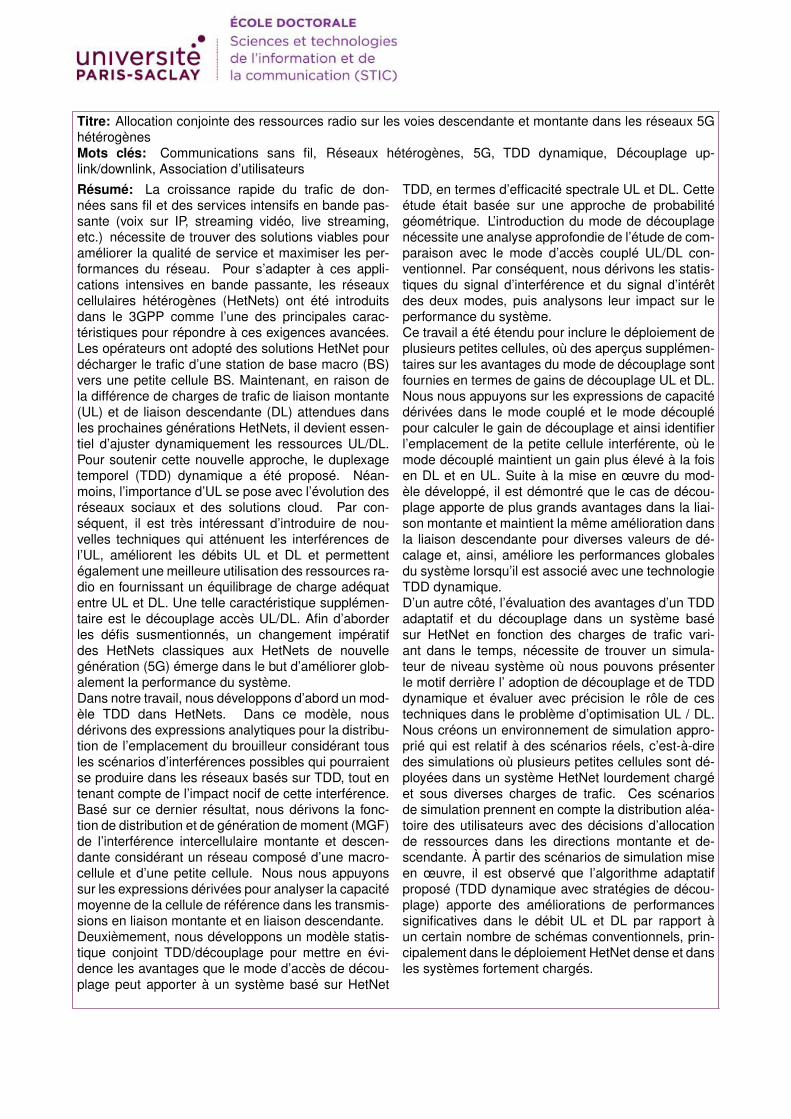
Titre: Allocation conjointe des ressources radio sur les voies descendante et montante dans les réseaux 5GhétérogènesMots clés: Communications sans fil, Réseaux hétérogènes, 5G, TDD dynamique, Découplage up-link/downlink, Association d’utilisateursRésumé: La croissance rapide du trafic de don-nées sans fil et des services intensifs en bande pas-sante (voix sur IP, streaming vidéo, live streaming,etc.) nécessite de trouver des solutions viables pouraméliorer la qualité de service et maximiser les per-formances du réseau. Pour s’adapter à ces appli-cations intensives en bande passante, les réseauxcellulaires hétérogènes (HetNets) ont été introduitsdans le 3GPP comme l’une des principales carac-téristiques pour répondre à ces exigences avancées.Les opérateurs ont adopté des solutions HetNet pourdécharger le trafic d’une station de base macro (BS)vers une petite cellule BS. Maintenant, en raison dela différence de charges de trafic de liaison montante(UL) et de liaison descendante (DL) attendues dansles prochaines générations HetNets, il devient essen-tiel d’ajuster dynamiquement les ressources UL/DL.Pour soutenir cette nouvelle approche, le duplexagetemporel (TDD) dynamique a été proposé. Néan-moins, l’importance d’UL se pose avec l’évolution desréseaux sociaux et des solutions cloud. Par con-séquent, il est très intéressant d’introduire de nou-velles techniques qui atténuent les interférences del’UL, améliorent les débits UL et DL et permettentégalement une meilleure utilisation des ressources ra-dio en fournissant un équilibrage de charge adéquatentre UL et DL. Une telle caractéristique supplémen-taire est le découplage accès UL/DL. Afin d’aborderles défis susmentionnés, un changement impératifdes HetNets classiques aux HetNets de nouvellegénération (5G) émerge dans le but d’améliorer glob-alement la performance du système.Dans notre travail, nous développons d’abord un mod-èle TDD dans HetNets. Dans ce modèle, nousdérivons des expressions analytiques pour la distribu-tion de l’emplacement du brouilleur considérant tousles scénarios d’interférences possibles qui pourraientse produire dans les réseaux basés sur TDD, tout entenant compte de l’impact nocif de cette interférence.Basé sur ce dernier résultat, nous dérivons la fonc-tion de distribution et de génération de moment (MGF)de l’interférence intercellulaire montante et descen-dante considérant un réseau composé d’une macro-cellule et d’une petite cellule. Nous nous appuyonssur les expressions dérivées pour analyser la capacitémoyenne de la cellule de référence dans les transmis-sions en liaison montante et en liaison descendante.Deuxièmement, nous développons un modèle statis-tique conjoint TDD/découplage pour mettre en évi-dence les avantages que le mode d’accès de décou-plage peut apporter à un système basé sur HetNet
TDD, en termes d’efficacité spectrale UL et DL. Cetteétude était basée sur une approche de probabilitégéométrique. L’introduction du mode de découplagenécessite une analyse approfondie de l’étude de com-paraison avec le mode d’accès couplé UL/DL con-ventionnel. Par conséquent, nous dérivons les statis-tiques du signal d’interférence et du signal d’intérêtdes deux modes, puis analysons leur impact sur leperformance du système.Ce travail a été étendu pour inclure le déploiement deplusieurs petites cellules, où des aperçus supplémen-taires sur les avantages du mode de découplage sontfournies en termes de gains de découplage UL et DL.Nous nous appuyons sur les expressions de capacitédérivées dans le mode couplé et le mode découplépour calculer le gain de découplage et ainsi identifierl’emplacement de la petite cellule interférente, où lemode découplé maintient un gain plus élevé à la foisen DL et en UL. Suite à la mise en œuvre du mod-èle développé, il est démontré que le cas de décou-plage apporte de plus grands avantages dans la liai-son montante et maintient la même amélioration dansla liaison descendante pour diverses valeurs de dé-calage et, ainsi, améliore les performances globalesdu système lorsqu’il est associé avec une technologieTDD dynamique.D’un autre côté, l’évaluation des avantages d’un TDDadaptatif et du découplage dans un système basésur HetNet en fonction des charges de trafic vari-ant dans le temps, nécessite de trouver un simula-teur de niveau système où nous pouvons présenterle motif derrière l’ adoption de découplage et de TDDdynamique et évaluer avec précision le rôle de cestechniques dans le problème d’optimisation UL / DL.Nous créons un environnement de simulation appro-prié qui est relatif à des scénarios réels, c’est-à-diredes simulations où plusieurs petites cellules sont dé-ployées dans un système HetNet lourdement chargéet sous diverses charges de trafic. Ces scénariosde simulation prennent en compte la distribution aléa-toire des utilisateurs avec des décisions d’allocationde ressources dans les directions montante et de-scendante. À partir des scénarios de simulation miseen œuvre, il est observé que l’algorithme adaptatifproposé (TDD dynamique avec stratégies de décou-plage) apporte des améliorations de performancessignificatives dans le débit UL et DL par rapport àun certain nombre de schémas conventionnels, prin-cipalement dans le déploiement HetNet dense et dansles systèmes fortement chargés.
Title:Joint Uplink/Downlink Radio Resource Allocation in 5G HetNets
Keywords: Wireless Communications, HetNets, 5G, Dynamic TDD, Uplink/Downlink Decoupling, User Asso-ciation
Abstract: The rapid growth in wireless data trafficand bandwidth intensive services (voice over IP, videostreaming, live streaming, etc.) necessitates find-ing viable solutions to improve service quality andmaximize the network performance. To accommo-date these bandwidth intensive applications, hetero-geneous cellular networks (HetNets) were introducedin 3GPP as one of the main features to meet these ad-vanced requirements. Operators have adopted Het-Net solutions to offload traffic from a macro base sta-tion (BS) to a small cell BS. Yet, because of the dif-ference in uplink (UL) and downlink (DL) traffic loadsexpected in the next HetNets generation, it becomesessential to dynamically adjust UL/DL resources. Tosupport this new approach, dynamic time-division du-plexing (TDD) has been proposed. Nevertheless, theimportance of UL arises along with the evolution ofsocial networking and cloud solutions. Therefore,it is of great interest to introduce novel techniquesthat mitigate UL interferences, improve UL and DLthroughputs and allow as well, a better use of radio re-sources by providing adequate load balancing amongUL and DL. Such an additional feature is the decou-pled UL/DL access. In order to address the aforemen-tioned challenges, an important shift from classicalHetNets to next-generation HetNets (5G) is emergingin the aim of improving overall system performance.In our work, we first develop a TDD model in HetNets.Under this model,we derive analytical expressions forthe distribution of the interferer location consideringall possible interference scenarios that could occur inTDD-based networks, while taking into account theharmful impact of interference. Based on the latterresult, we derive the distribution and moment gener-ating function (MGF) of the uplink and downlink inter-cell interference considering a network consisting ofone macro cell and one small cell. We build on thederived expressions to analyze the average capacityof the reference cell in both uplink and downlink trans-missions.Second, we develop a joint TDD/decoupling statisti-cal model to highlight the benefits that the decouplingaccess mode can bring to a HetNet TDD based sys-
tem, in terms of UL and DL spectral efficiencies andthroughputs. This study was based on a geomet-ric probability approach. Introducing the decouplingmode necessitates a thorough comparison study withthe conventional coupled UL/DL access mode. There-fore, we derive the statistics of the interference signaland the signal of interest of both modes and then an-alyze their impact on the system performance.This work was extended to include multiple small cellsdeployment, where more insight into the benefits ofdecoupling mode is provided in terms of UL and DLdecoupling gains. We build on the derived capacityexpressions in the coupled and decoupled modes tocalculate the decoupling gain and thus, identify thelocation of the interferer small cell where the decou-pled mode maintains a higher gain in both DL andUL. Further to the implementation of the developedmodel, it is shown that the decoupling case bringsgreater benefits in the uplink and maintains the sameimprovement in the downlink for various offset valuesand thus, improves the overall system performancewhen being combined with a dynamic TDD technol-ogy.On the other hand, evaluating the benefits of an adap-tive TDD and decoupling in a HetNet based sys-tem according to time-variant traffic loads, necessi-tates finding a system level simulator where we canpresent the motivation and accurately assess the roleof both decoupling and dynamic TDD techniques inthe UL/DL optimization problem. We create appro-priate simulation environment that is relative to realscenarios i.e. simulations where multiple small cellsare deployed in a heavy loaded HetNet system andunder various traffic loads. These simulation scenar-ios consider random users distribution with schedulingdecisions in both the uplink and the downlink direc-tions. From the applied simulation scenarios, it is ob-served that the proposed adaptive algorithm (dynamicTDD with decoupling policies) yields significant perfor-mance improvements in UL and DL throughput com-pared to a number of conventional schemes, mainlyin dense HetNet deployment and in highly loaded sys-tems.
Université Paris-SaclayEspace Technologique / Immeuble DiscoveryRoute de l’Orme aux Merisiers RD 128 / 91190 Saint-Aubin, France
Recommended