Procedia CIRP 7 ( 2013 ) 347 – 352

2212-8271 © 2013 The Authors. Published by Elsevier B.V.Selection and peer-review under responsibility of Professor Pedro Filipe do Carmo Cunhadoi: 10.1016/j.procir.2013.05.059

Forty Sixth CIRP Conference on Manufacturing Systems 2013

Learning defect classifiers for textured surfaces using neural networks and statistical feature representations

D. Weimera*, H. Thamera, B. Scholz-Reiterb aIntelligent Production Systems (BIBA), University of Bremen, Hochschulring 20, 28359 Bremen, Germany

b University of Bremen, Bibliotheksstraße 1, 28359 Bremen, Germany * Corresponding author. Tel.: +49(0) 421-218-50181; fax: +49(0)421-218-50003; E-mail address: wei@biba.uni-bremen.de.

Abstract

Detecting surface defects is a challenging visual recognition problem arising in many processing steps during manufacturing. These defects occur with arbitrary size, shape and orientation. The challenges posed by this complexity have been combated with very special, runtime intensive and hand-designed feature representations. In this paper we present a machine vision system which uses basic patch statistics from raw image data combined with a two layer neural network to detect surface defects on arbitrary textured and weakly labeled image data. Evaluation on an artificial dataset with more than 6000 examples in addition to a real micro-cold forming process showed excellent classification results. © 2013 The Authors. Published by Elsevier B.V. Selection and/or peer-review under responsibility of Professor Pedro Filipe do Carmo Cunha Keywords: Defect Classifier, Surface Inspection, Neural Networks, Micro Production

1. Introduction

Non-destructive visual analysis of textured surfaces is a common application for machine vision systems. They are concerned with recognizing patterns to distinguish between defect and non-defect classes. In manufacturing scenarios such vision systems have to be reliable, accurate and fast. In many cases visual inspection is still realized by humans with respect to the high detection rate but limited by inspection frequency and costs. Focusing all this issues often results in very problem specific automated solutions with highly optimized feature representations for defect and non-defect regions. A very challenging application in visual inspection deals with strong textured materials. Common criteria to qualify textured materials are isotropy, homogeneity and coarseness [1]. Simple algorithms are often not sufficient in the strong textured case, because background texture is very strong compared to the defect region. In many cases there is not much difference between background texture and defect area.

Detecting such local texture anomalies is one of the important research topics in machine vision [2]. Xie

divided the methods for textural defect detection in four main categories: statistical, structural, filter based and model based [3]. The focus in this paper is set to statistical and model based techniques. Statistical texture representation methods measure the distribution of pure pixel values inside a specific image region. Well known techniques are histograms [4-5], co-occurrence matrices [6-7] and local binary patterns [8-9].

Focusing inspection scenarios with prior information about defect parameters or a sufficient quantity of training data, supervised machine learning methods can be applied to learn a detection model. Kumar used a macro-window approach in combination with principal component analysis (PCA) for feature generation to train a feed forward neural network and successfully applied it to fabric scenarios [10]. In [11] a combination of binary tree-based support vector machine (SVM) structures showed good results in welding defect detection. Filter bank techniques in combination with an unsupervised learning method where introduced by Leung and Malik for reliable texture recognition and categorization [12]. Based on this work Xie and Mirmehdi introduced the TEXEM model which deals with image patches of arbitrary size and generates

Available online at www.sciencedirect.com

© 2013 The Authors. Published by Elsevier B.V.Selection and peer-review under responsibility of Professor Pedro Filipe do Carmo Cunha

348 D. Weimer et al. / Procedia CIRP 7 ( 2013 ) 347 – 352

Gaussian mixture models in a hierarchical two-layer fashioned learning procedure [13]. Another neuralnetwork technique driven by evolutionary reinforcement learning was proposed by Siebel and Sommer [14]. They compare two different feature architectures andevaluated them on an artificial benchmark dataset. In[18] a method was introduced using Eigenchannels and amixture model to find defect patterns in textured images.

The method introduced in this paper presents a very basic feature description combined with a two layer neural network representation. Features are generated by combining multi-resolution analysis and grayscale patchstatistics. In an offline training procedure a neuralnetwork trains a model based on randomly selectedimage pages to separate background from defect regionand applies this model to unknown examples. Different parameter settings of the proposed technique will beevaluated and compared with the same dataset as used in [14]. In a final case study, we apply the framework to areal micro-cold forming scenario by inspecting metallicmicro cups. Thereby, image acquisition is realized byconfocal laser microscopy. The method shows good detection performance on artificial texture databases andin real manufacturing processes.

2. Defect Detection Method

The proposed detection scheme in Fig. 1 is composedof two major sections. In an offline training mode thealgorithm uses a dataset of labeled training examples with and without defect regions and extracts random patches of size s = N×N, NN where N is the number of pixel in x-and y direction. If a patch is part of a defect regionthe label y is set to 1 and 0 vice versa. The extraction of statistical values which describe each single patch is part of the feature calculation step. Each single image patchis now represented by a feature vector withcorresponding defect label (x,y), where X={xXX (1) (m)}) isa matrix containing all m training examples as row vectors. In the last step the neural network classifier usesall training examples X to learn a hypothesis (model) h(x) via backpropagation learning procedure.

The training procedure runs in an offline mode.Therefore it is not related to any runtime constraints. Theevaluation of unknown examples without label isrealized in sliding window vice fashion. The complete image is divided into overlapping blocks of size s where the overlap is s/2ss in x and y direction. The learned neuralnetwork model uses the extracted statistical features andpredicts whether an image patch belongs to the defect or non-defect class.

In some cases the algorithm classifies individualimage pages as defective, although there are defect free.Therefore, we use a non-maxima suppression technique

to adjust incorrect local classification results. A finalvisualization step marks all classified defect areas.

2.1. Feature Extraction

The set of features extracted from raw image data iscrucial for final classification results. To keep theframework simple we use basic statistical features based on grayscale values inside the image patches. Fig. 2shows the overall method for feature extraction andmodel learning. Instead of using the complete image astraining example we extract a fixed number of patches pwith size s from each image as demonstrated in theRandom patch generation part of Fig. 2. The next stepPatch layout shows the overall representation of raw image patches where each image patch is now represented as a row vector. Note that (x(i(( )i ,y(i))) representsthe i-th training example with the corresponding imagelabel 1 (defect) or 0 (non-defect). It is common practiceto apply basic normalization procedures beforeextracting patch features [15]. The result is a representation of the training example vectors in a range of [0,1].

After normalization, statistical features are calculated to represent an image patch. The feature generation steptakes the training data X and outputs a function f: N×N D which maps each single training examplex(i)xx from a N×N dimensional to a D dimensional space. The value of D is a parameter of the framework and represents the number of statistical features. Besides

Fig. 1. Defect detection framework structure

Offline Training

Extract ImagePatches

GeneratingStatistical Featut res

Laba elled Dataset

Tra

inin

g D

ata

Feat

ures

Tra

inin

g

Sliding WindowExtraction

Evaluation D

ataE

valuation

Train NeuralNetwork

Generating StatisticalFeatut res

MMMoodddeelll

Online Evaluation

DDeeffeeffff cctt OOKK

Non-maximaSuppu ppression

349 D. Weimer et al. / Procedia CIRP 7 ( 2013 ) 347 – 352

features like mean, median and standard deviation (std), we use central moments from 2nd to 5th order. The central moment mk of order k of a grayscale image patch is calculated by

(1)

where E(x(i)) is the expected value of x(i). Other moments used for feature representation in this paper are Hu-moments [16]. This seven rotation invariant features are derivations and combinations of the basic central moments. The calculation of statistical image features on raw image patches reduces the feature dimension from N×N to D=15 elements for each training example vector x(i). This is the final feature dimension and the input values to the neural network training algorithm.

2.2. Learning Defect Classifier

In the previous feature calculation step we mapped the features to a new representation f D. Now we use the labeled training data to train a neural network using backpropagation. An example of a neural network structure is shown in Fig. 2 Feature classification. The size of the input layer is equal to the feature dimension, here k=15. The second layer, called the hidden layer, has L1 nodes. In the output layer, all nodes from the hidden layer are mapped to one final node showing the classification result. All weights in the neural network are initialized by random numbers. Training a network means optimizing network detection performance. This is realized by minimizing the performance function. The performance measurement function in this case is the mean squared error (MSE). Other techniques for network optimization are discussed in [20]. We used MSE minimization because it performed best in this

scenario. The MSE measures the averaged squared error between the network output (layer L2) h(x) and the labels of the training examples y. MSE is defined as:

(2)

After training, the algorithm outputs the weight

matrix W and the additional biases b. The weight matrix W has the size D×L1 and the bias vector b 1×L1. Every unknown example can be classified by calculating the feature hypotheses h(x) by

(3)

where g(z)=1/(1+exp(-z)) is called the sigmoid function and is applied component-wise to the vector z. The final classification result is a value between [0, 1] and predicts whether an unknown image patch contains defect regions or not.

3. Experiments and Analysis

3.1. Dataset

The dataset used in this work is provided by the German Association for Pattern Recognition (DAGM) and the European Neural Network Society (GNNS) [17]. We refer to it in the following as DAGM dataset. The dataset consists of 6 different classes with 150 positive examples (defect) and 1000 negative examples (non-defect). These are more than 6500 examples in total with an image size of 512px×512px each. The images inside a single class are similar but all examples have a very strong background texture and varying kinds of defects. Examples from each are shown in Fig. 4. In many cases

m

i

ii yxhm

MSE1

)()( ))((1

bWxgxh

...

Number of training examples n

Random patch generation

N

N

Patch layout

(x(1),y)

...

N× N

... ...

... ... ...

... ... ...

... ... ...

# patch per image

n

Feature classification

... ...

L1 L2

...

123

d

...

Patchstatistics

...

kiik xEm )/)(

Fig 2. Patch extraction, feature representation and learning procedure

350 D. Weimer et al. / Procedia CIRP 7 ( 2013 ) 347 – 352

it is hard to detect the defect region, even with human eyes. The dataset provides weak labels for each training example to mark the defect. This means, that a label area contains not just defect pixel, but also very much background pixel which makes it even harder for an algorithm to separate defect from non-defect class.

3.2. Detection Performance

Instead of using the whole image for feature extraction, we are using random patch generation. To find the best patch size s=N×N, we evaluated 3 different arrangements starting from s=7×7 were the distribution of pixel values is very coarse. Additionally we used s=20×20 and s=32×32 which corresponds to a more significant statistical gray-scale value distribution inside each patch.

A common strategy is to divide a dataset in training data and evaluation data. Here, 70% of the negative and positive image data are used for training and 30 % are used for evaluation. To get positive training data (with defect) we randomly extracted 1500 patches of size s from labeled image areas for each class and 600 patches for evaluation. In the negative case for non-defect images the total number of training examples is 5000 and 1800 for evaluation.

The sub-parameters for the optimal configuration of the neural network are optimized using grid search. The hidden layer size in the neural network is L1 = 25. We evaluated this value by experiments and selected it as a tradeoff between computation time and classification

accuracy. Neural networks tend to overfitting during training procedure which results in a very specific problem model. With respect to better classification performance using unknown examples we use early stopping criteria to optimize generalization of the neural network model [19].

To measure the detection performance of the learned model we use ROC analysis (Receiver Operating Characteristic). ROC space is defined with the false positive rate (fpr) on the x-axis and true positive rate (tpr) on the y-axis. Here, tpr is the ratio of correct detected defects TP with respect to the total number of defect images P, tpr=TP/P. The fpr shows the ratio of defect free images incorrectly classified as defective FP with respect to the total number of defect free images N (fall-out), fpr=FP/N. The ROC curve is ideal, if the area under the curve is approximately one, and therefore if the curve is in the north-west of the ROC graph.

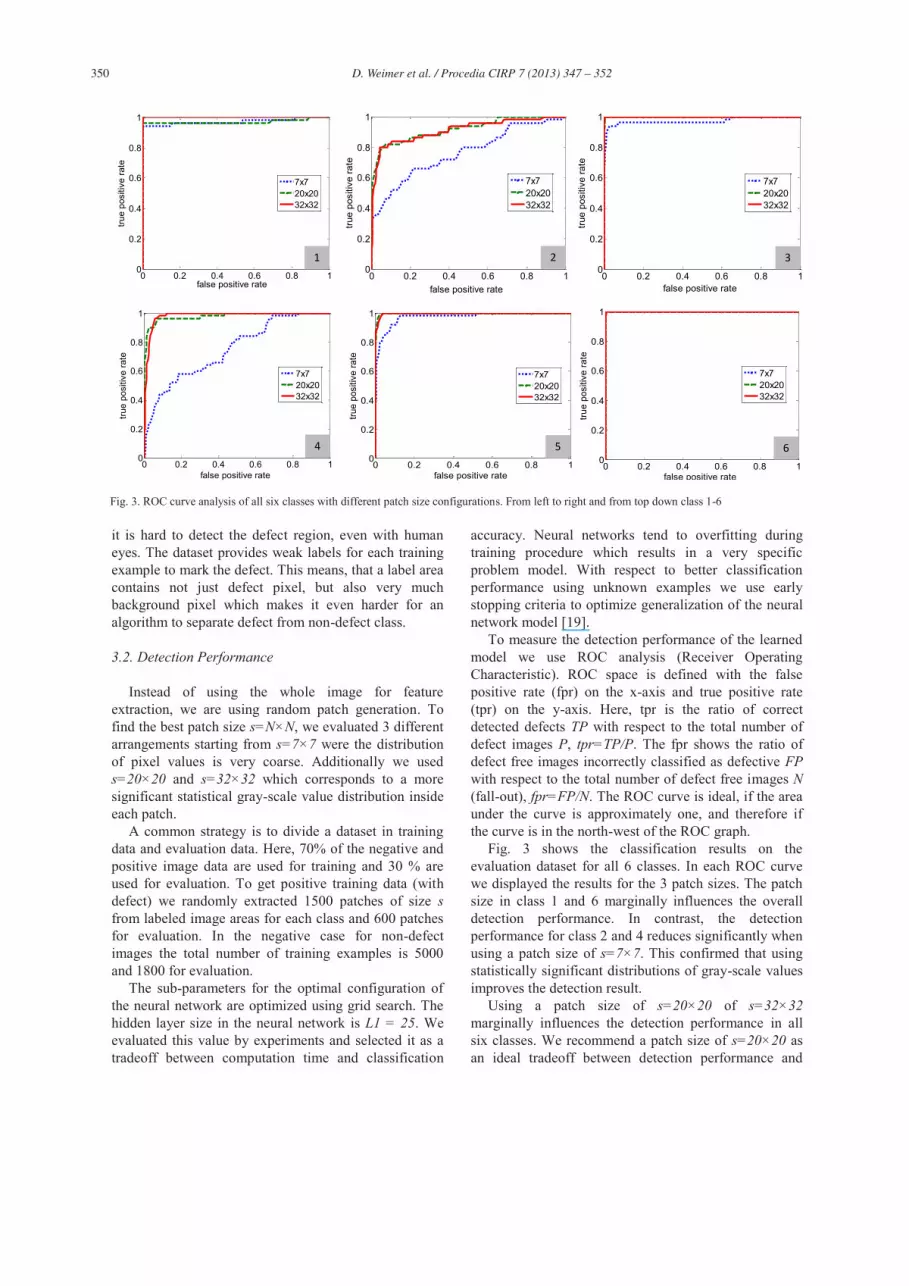
Fig. 3 shows the classification results on the evaluation dataset for all 6 classes. In each ROC curve we displayed the results for the 3 patch sizes. The patch size in class 1 and 6 marginally influences the overall detection performance. In contrast, the detection performance for class 2 and 4 reduces significantly when using a patch size of s=7×7. This confirmed that using statistically significant distributions of gray-scale values improves the detection result.

Using a patch size of s=20×20 of s=32×32 marginally influences the detection performance in all six classes. We recommend a patch size of s=20×20 as an ideal tradeoff between detection performance and

Fig. 3. ROC curve analysis of all six classes with different patch size configurations. From left to right and from top down class 1-6

0 0.2 0.4 0.6 0.8 10

0.2

0.4

0.6

0.8

1

false positive rate

true

posi

tive

rate

7x720x2032x32

0 0.2 0.4 0.6 0.8 10

0.2

0.4

0.6

0.8

1

false positive rate

true

posi

tive

rate

7x720x2032x32

0 0.2 0.4 0.6 0.8 10

0.2

0.4

0.6

0.8

1

false positive rate

true

posi

tive

rate

7x720x2032x32

0 0.2 0.4 0.6 0.8 10

0.2

0.4

0.6

0.8

1

false positive rate

true

posi

tive

rate

7x720x2032x32

0 0.2 0.4 0.6 0.8 10

0.2

0.4

0.6

0.8

1

false positive rate

true

posi

tive

rate

7x720x2032x32

0 0.2 0.4 0.6 0.8 10

0.2

0.4

0.6

0.8

1

false positive rate

true

posi

tive

rate

7x720x2032x32

1 2 3

4 5 6

351 D. Weimer et al. / Procedia CIRP 7 ( 2013 ) 347 – 352

(a) Class 1: original label (120) (b) Class 1: detection result (d) Class 2: detection result(c) Class 2: original label (10)

(e) Class 3: original label (87) (f) Class 3: detection result (g) Class 4: original label (13) (h) Class 4: detection result

(i) Class 5: original label (58) (j) Class 5: detection result (k) Class 6: original label (143) (l) Class 6: detection result

runtime. Fig. 4 shows detection examples of the DAGM dataset, where a complete image of size 512px×512px is analyzed in sliding window vice fashion by shifting a window of patch size s=20×20 over the image with a window stride of half patch size (s/2) in x and y direction. The neural network evaluates each patch (procedure see Fig. 1) and positive (defect) patches are visualized with yellow rectangles. To avoid single hits, we apply mean shift, witch clusters all detected rectangles and deletes very small clusters (1-3 hits). Note that in some cases (e.g. class 4) not each pixel of the defect is classified as defective, but a major part of the defect.

4. Case Study

The statistical features combined with a neural network works very well on the artificial DAGM dataset. To demonstrate real world suitability we focus on a real micro cold forming scenario, where a micro cold forming machine produces micro cups [20]. The

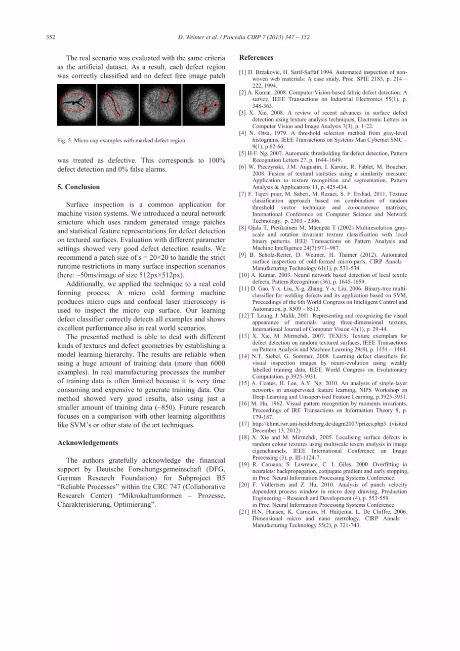
micro cups (aluminum) have a diameter of 800 μm and a height of 500 μm. Confocal laser microscopy (Keyence VK-9700-3D) is used as metrology since it performs very well in the micro range [21]. The focus of the metrology is set to the bottom of the micro cup as shown in Fig. 5. Red ellipses mark the defective regions. The kinds of defects vary from cracks, dents up to soiling and vary in size, shape and orientation [9].

The dataset consists of 67 images with defect and 106 without defect. The image resolution is 1024px×1024px. Based on the higher image resolution we also increased the patch size to s=32×32. We extracted 250 positive patches (with defect) and 620 negative patches for training and 100 positive and 250 negative patches for evaluation. As before, the dataset is divided into a training set and an evaluation set. The same holds for the generation of random patches. Statistical features are used for training and the size of the hidden layer is L1=25.

Fig. 4: Detection examples from all classes. In column order, class 1 to class 6. Ellipses in red mark the original weak label, yellow areas mark detection results based on neural network classification. Numbers in brackets show image number in database (runtime ~ 50 ms/image)

352 D. Weimer et al. / Procedia CIRP 7 ( 2013 ) 347 – 352

The real scenario was evaluated with the same criteria

as the artificial dataset. As a result, each defect region was correctly classified and no defect free image patch

was treated as defective. This corresponds to 100% defect detection and 0% false alarms.

5. Conclusion

Surface inspection is a common application for machine vision systems. We introduced a neural network structure which uses random generated image patches and statistical feature representations for defect detection on textured surfaces. Evaluation with different parameter settings showed very good defect detection results. We recommend a patch size of s = 20×20 to handle the strict runtime restrictions in many surface inspection scenarios (here: ~50ms/image of size 512px×512px).

Additionally, we applied the technique to a real cold forming process. A micro cold forming machine produces micro cups and confocal laser microscopy is used to inspect the micro cup surface. Our learning defect classifier correctly detects all examples and shows excellent performance also in real world scenarios.

The presented method is able to deal with different kinds of textures and defect geometries by establishing a model learning hierarchy. The results are reliable when using a huge amount of training data (more than 6000 examples). In real manufacturing processes the number of training data is often limited because it is very time consuming and expensive to generate training data. Our method showed very good results, also using just a smaller amount of training data (~850). Future research focuses on a comparison with other learning algorithms

Acknowledgements

The authors gratefully acknowledge the financial support by Deutsche Forschungsgemeinschaft (DFG, German Research Foundation) for Subproject B5

he CRC 747 (Collaborative Mikrokaltumformen Prozesse,

Charakterisierung, Optimierung .

References

[1] D. Brzakovic, H. Sarif-Saffaf 1994. Automated inspection of non-woven web materials: A case study, Proc. SPIE 2183, p. 214 222, 1994.

[2] A. Kumar, 2008. Computer-Vision-based fabric defect detection: A survey, IEEE Transactions on Industrial Electronics 55(1), p. 348-363.

[3] X. Xie, 2008. A review of recent advances in surface defect detection using texture analysis techniques, Electronic Letters on Computer Vision and Image Analysis 7(3), p. 1-22.

[4] N. Otsu, 1979. A threshold selection method from gray-level histograms, IEEE Transactions on Systems Man Cybernet SMC 9(1), p 62-66.

[5] H-F. Ng, 2007. Automatic thresholding for defect detection, Pattern Recognition Letters 27, p. 1644-1649.

[6] W. Pieczynski, J.M. Augustin, I. Karoui, R. Fablet, M. Boucher, 2008. Fusion of textural statistics using a similarity measure: Application to texture recognition and segmentation, Pattern Analysis & Applications 11, p. 425-434.

[7] F. Tajeri pour, M. Saberi, M. Rezaei, S. F. Ershad, 2011, Texture classification approach based on combination of random threshold vector technique and co-occurence matrixes, International Conference on Computer Science and Network Technology, p. 2303 - 2306.

[8] Ojala T, Pietikäinen M, Mäenpää T (2002) Multiresolution gray-scale and rotation invariant texture classification with local binary patterns. IEEE Transactions on Pattern Analysis and Machine Intelligence 24(7):971 987.

[9] B. Scholz-Reiter, D. Weimer, H. Thamer (2012). Automated surface inspection of cold-formed micro-parts, CIRP Annals Manufacturing Technology 61(1), p. 531-534.

[10] A. Kumar, 2003. Neural network based detection of local textile defects, Pattern Recognition (36), p. 1645-1659.

[11] D. Gao, Y-x. Liu, X-g. Zhang, Y-x. Liu, 2006. Binary-tree multi-classifier for welding defects and its application based on SVM, Proceedings of the 6th World Congress on Intelligent Control and Automation, p. 8509 8513.

[12] T. Leung, J. Malik, 2001. Representing and recognizing the visual appearance of materials using three-dimensional textons, International Journal of Computer Vision 43(1), p. 29-44.

[13] X. Xie, M. Mirmehdi, 2007. TEXES: Texture exemplars for defect detection on random textured surfaces, IEEE Transactions on Pattern Analysis and Machine Learning 29(8), p. 1454 1464.

[14] N.T. Siebel, G. Sommer, 2008. Learning defect classifiers for visual inspection images by neuro-evolution using weakly labelled training data, IEEE World Congress on Evolutionary Computation, p.3925-3931.

[15] A. Coates, H. Lee, A.Y. Ng, 2010. An analysis of single-layer networks in unsupervised feature learning, NIPS Workshop on Deep Learning and Unsupervised Feature Learning, p.3925-3931.

[16] M. Hu, 1962. Visual pattern recognition by moments invariants, Proceedings of IRE Transactions on Information Theory 8, p. 179-187.

[17] http://klimt.iwr.uni-heidelberg.de/dagm2007/prizes.php3 (visited December 13, 2012)

[18] X. Xie and M. Mirmehdi, 2005. Localising surface defects in random colour textures using multiscale texem analysis in image eigenchannels, IEEE International Conference on Image Processing (3), p. III-1124-7.

[19] R. Caruana, S. Lawrence, C. L Giles, 2000. Overfitting in neuralets: backpropagation, conjugate gradient and early stopping, in Proc. Neural Information Processing Systems Conference.

[20] F. Vollertsen and Z. Hu, 2010. Analysis of punch velocity dependent process window in micro deep drawing, Production Engineering Research and Development (4), p. 553-559.

in Proc. Neural Information Processing Systems Conference [21] H.N. Hansen, K. Carneiro, H. Haitjema, L. De Chiffre, 2006.

Dimensional micro and nano metrology. CIRP Annals Manufacturing Technology 55(2), p. 721-743.

Fig. 5: Micro cup examples with marked defect region