Download pdf - Mapping landfill gas migration using resistivity monitoring

Delivered by ICEVirtualLibrary.com to:

IP: 130.235.33.187

On: Wed, 17 Aug 2011 15:56:23

Waste and Resource ManagementVolume 164 Issue WR1

Mapping landfill gas migration usingresistivity monitoringRosqvist et al.

Proceedings of the Institution of Civil Engineers

Waste and Resource Management 164

February 2011 Issue WR1

Pages 3–15 doi: 10.1680/warm.2011.164.1.3

Paper 900026

Received 22/09/2009 Accepted 15/02/2010

Keywords: landfill/site investigation/waste management

& disposal

ICE Publishing: All rights reserved

Mapping landfill gas migrationusing resistivity monitoringHakan Rosqvist PhD

Researcher, Research Department, NSR AB, Helsingborg, Sweden

Virginie Leroux PhD

Research Associate, Engineering Geology, Lund University, Lund, Sweden

Torleif Dahlin PhD

Associate Professor, Engineering Geology, Lund University, Lund, Sweden

Mats Svensson PhD

Head of GEO Department, Tyrens AB, Helsingborg, Sweden

Magnus Lindsjo MSc

Environmental Engineering, Research Department, NSR AB, Helsingborg,

Sweden

Carl-Henrik Mansson MSc

Environmental Engineering, Tyrens AB, Helsingborg, Sweden

Sara Johansson MSc

Biogeophysics, Department of Physics, Lund University, Lund, Sweden

Results of geoelectrical resistivity monitoring at two landfill sites, a bioreactor landfill and a conventional municipal

solid waste landfill site over a week are reported. The main objective was to investigate if geoelectrical resistivity can

be used for localising paths for landfill gas migration. The resistivity results were also related to local pore pressure

measurements and to methane emission measurements using a laser-scanning instrument. The results suggest that the

use of the interpreted resistivity and of its temporal variation can be suitable for the intended purpose, and confirm

the applicability of resistivity imaging at landfills. It is also concluded that better knowledge about the dependence of

resistivity variation to temperature, porosity and moisture content variations would improve the interpretation and

that measuring or monitoring at least one of these additional parameters together with resistivity would be useful.

1. IntroductionControl and estimation of landfill gas emissions have become a

major concern in landfill management, since, apart from the

risks of fire and explosion and the odour nuisance, methane is

a powerful greenhouse gas. Its effect is more than 20 times

that of carbon dioxide, and landfills are regarded as one of

the major anthropogenic sources (O’Leary and Walsh, 2002).

The concentration of methane in landfill gas varies, often in a

range between 40 and 60%, constituting an interesting energy

resource as it can be used for heating and power generation.

In recent years the development of upgrading techniques for

landfill gas to vehicle fuel has further increased the interest for

landfill gas utilisation. A large number of landfills, closed or

active, are equipped with gas-collecting systems. However,

their efficiency is often limited. In many parts of the world

legislation requires measures for limiting gas emissions to the

atmosphere and often also reporting of the gas emissions

(Ljungberg et al., 2008).

Attempts have been made to estimate the total gas emissions

at landfills and to identify the areas with higher rates. With

this purpose several techniques have been tested, for example

infrared cameras, laser scanning and chambers for measuring

the methane flux at the surface (see e.g. Ljungberg et al.,

2008). It has been pointed out that this is a difficult task even

if the techniques have been shown to be useful. None of them

can be regarded as entirely satisfactory. Furthermore, no

information about what is happening inside the landfill can be

reported in that way. Zones with higher emission rates can be

identified on the surface, such as, for example, slopes, where

cracks easily open (see e.g. Ljungberg et al., 2008), but the

origin and the paths taken by the gas inside a landfill are not

obvious.

Owing to the heterogeneous structure of municipal solid

waste (MSW) landfills decomposition processes are highly

non-uniform, resulting in variable gas generation rates at

different locations in a landfill. The decomposition processes

are, for example, dependent on the moisture content and the

evolution degree of degradable waste.

Because a landfill is often constructed as a succession of

horizontally compacted layers, the permeability is generally

higher in the horizontal direction. However, other physical

heterogeneities such as fissures also cause a non-uniform flow

of gas following the path of least resistance. Thus, the processes

involved in landfill gas generation and migration are complex,

and they are controlled by a number of parameters: the

temperature, the concentration of oxygen, the atmospheric

pressure and the moisture content at depth, in the topsoil and

in the air.

The electrical resistivity of an earth-like material depends on the

ratio of the gas and water volume in the pores, as well as on

the temperature, the salinity of the pore fluid and on the overall

porosity. Generally speaking, the equations to consider depend

3


IP: 130.235.33.187

On: Wed, 17 Aug 2011 15:56:23

on the kind of current conduction involved: through the ions

and particles present in the pore water, by way of surface con-

duction and on their relative importance. Archie’s Equation

(Archie, 1942) takes only the first kind of processes into

account. It can be expressed for the unsaturated medium as

¼ amwSnw1.

where is the electrical resistivity, w the resistivity of the pore

water, the porosity, Sw the saturation defined as the ratio of

the volume of pore water to the total pore volume. The constant

a lies generally between 0.6 and 1, the cementation exponent m

generally lies between 1.4 and 2.2 in common rocks and the

saturation exponent is close to 2 (e.g. Ward, 1990). This

equation has been used for MSW material (Grellier, 2005),

where the conductivity of the pore water is generally high. Its

relative simplicity makes it attractive. Nevertheless, it might

not be entirely satisfactory for waste materials where the surface

conduction can be expected to be relatively important. An

indication for that is the high induced polarisation usually

measured on municipal landfills (see e.g. Carlson et al., 1999;

Dahlin et al., 2002; Leroux et al., 2007). Other models such as

the equation proposed by Waxman and Smits (1968) might

then better describe the electrical resistivity in such materials.

However, this kind of empirical model requires calibration

with laboratory data to assign values to the different parameters

(see e.g. Mavko et al., 2009). Very little data is available at

present that concerns waste materials, and the heterogeneity

in waste will probably render predictions difficult.

The resistivity furthermore depends on the temperature, follow-

ing an equation given by Keller and Frischknecht (1966)

t ¼18

1þ ðt 18Þ2.

where t is the temperature in 8C, 18 is the resistivity at 188C, tthe resistivity at the temperature t and is a constant depending

on the material considered and on the pore water composition.

It is classically given as ¼ 0.025 per 8C (Ward, 1990). Grellier

et al. (2006) have shown that this equation is applicable for the

leachate found in MSW, with comparable values for , slightly

depending on the type of ions present in the leachate, their

concentration as well as the concentration in solid particles in

suspension.

The conduction of electricity in MSW is a complex phenom-

enon, depending on several parameters. A more precise descrip-

tion of their influence requires laboratory measurements and

experimentations, as reported for example in Moreau et al.

(2008). Consequently, the resistivity alone cannot be directly

translated into a gas or methane concentration of the material.

But the presence of a certain amount of gas is likely to influence

the material’s resistivity, because of the change in temperature,

humidity and possibly porosity induced. Especially gas emis-

sions have been observed to be intermittent, showing that the

changes vary considerably with time (Ljungberg et al., 2008).

The paths taken by the migrating gas could then be detected

by monitoring resistivity; that is by mapping its variations

with time. The time scale to consider lies probably in the

range from a few hours to a few days.

Electrical resistivity imaging is a relatively well-known method

and has been used for a number of landfill applications. Its

principles are described in, for example, Zonge et al. (2005).

In short, a number of electrical potentials are measured between

pairs of electrodes while transmitting current between two other

electrodes. A large number of electrodes positions are used so as

to provide an adequate coverage of the volume. In practice it is,

however, often only possible to place the electrodes on the

ground surface. Since landfills are very heterogeneous media it

is appropriate to try to create a three-dimensional (3D) image

by placing the electrodes on a grid and measuring along parallel

lines. The measurements are processed by inversion to produce

the image, which generally consists in iterative computations

aiming at finding a realistic resistivity model with a numerical

response sufficiently close to the one measured.

In a field experiment conducted in 2007 at the Filborna landfill

in Sweden, resistivity was measured at several locations with

stationary electrodes placed on 11 parallel lines. Simultaneously,

the methane concentration at the surface was measured using a

laser-scanning unit, and methane flux at discrete locations was

measured by the static chamber method. The measurement

showed zones where large resistivity variations were clearly cor-

related with zones of high gas emissions (Dahlin et al., 2008).

Prior to that, growing resistive anomalies had been observed

under experiments of leachate recirculation at bioreactors, and

they had been interpreted as gas accumulation and migration

(e.g. Rosqvist et al., 2005; 2007).

These considerations led the present authors to conduct two

large-scale monitoring experiments at two different landfill

sites producing landfill gas. Two experiments of resistivity

monitoring were conducted at two sites: a bioreactor landfill

and a conventional MSW landfill. 3D models of resistivity

and resistivity variability were compared with gas pressure at

depth and with methane concentration at the surface using a

laser-scanning technique.

2. Material and method2.1 Resistivity monitoring

In the two field experiments geophysical resistivity monitoring

was carried out with the ABEM Lund imaging system. Nine

parallel lines of electrodes were set up. Each line was 20m



4

https://www.researchgate.net/publication/215755936_The_Rock_Physics_Handbook_Tool_for_Seismic_Analysis_in_Porous_Media?el=1_x_8&enrichId=rgreq-391527ea-7651-4631-9f83-7860361c7306&enrichSource=Y292ZXJQYWdlOzI3MzkzODM2ODtBUzoyMTA3NjUxOTg5NTg1OTNAMTQyNzI2MTc0Nzk1Mg==

https://www.researchgate.net/publication/273337271_Resistivity_and_induced_polarization_methods?el=1_x_8&enrichId=rgreq-391527ea-7651-4631-9f83-7860361c7306&enrichSource=Y292ZXJQYWdlOzI3MzkzODM2ODtBUzoyMTA3NjUxOTg5NTg1OTNAMTQyNzI2MTc0Nzk1Mg==

https://www.researchgate.net/publication/273337271_Resistivity_and_induced_polarization_methods?el=1_x_8&enrichId=rgreq-391527ea-7651-4631-9f83-7860361c7306&enrichSource=Y292ZXJQYWdlOzI3MzkzODM2ODtBUzoyMTA3NjUxOTg5NTg1OTNAMTQyNzI2MTc0Nzk1Mg==


IP: 130.235.33.187

On: Wed, 17 Aug 2011 15:56:23

long with 21 electrodes placed regularly every 1m. The lines

were equally spaced with 2m between them. The array used

for the measurements was the pole–dipole, in both forward

and reverse configurations. Each site was monitored succes-

sively during one week with a remote-controlled system, with

automatic data transfer to a server at Lund University for

data processing and inverse modelling. The time for the 50%

duty injection cycle was 1 s, which is sufficiently short to make

it possible to measure all the lines (3888 measurements) within

about 1 h and 45min, and also sufficiently long to allow for

the potential to stabilise. Charge-up and polarisation effects

are notoriously important at landfills (Carlson et al. 1999;

Dahlin et al. 2002; Leroux et al. 2007) and measuring too

hastily can result in underestimating the resistivity. The data

have to be processed by inversion before a resistivity image of

the studied area can be produced. All data for each complete

set of measurements were inverted together using Res3Dinv

(Loke and Barker, 1996; Loke, 2008). A true 3D model was

computed independently for each time-step, using the same

parameters and the same grid geometry. The L1-norm or

robust inversion method was used, which implies the minimi-

sation of the absolute discrepancy between the measured and

the computed data. This method is less sensitive to noise and

is able to reconstruct models with sharp boundaries (Loke

et al., 2003).

A single resistivity image accounts for the overall structure at the

landfill, but resistive anomalies cannot be directly interpreted as

mainly due to landfill gas, since higher resistivity can be attribu-

ted to other causes, as discussed above. It is not clear whether the

presence of landfill gas should always result in higher resistivity

either. Therefore, the present authors have chosen to interpret

a single resistivity image in terms of the structure of the landfill,

and to interpret the variation of resistivity with time as an

indicator of the presence and migration of landfill gas. In some

cases the variation of resistivity might confirm what can be

suspected from the landfill structure, but new features might

also be detected. To estimate the variations of resistivity during

the monitored period, the variation coefficient (Cv) has simply

been computed for all the inverted models and calculated as

Cv ¼

3.

where is the mean resistivity value for one cell and is the

standard deviation given by

¼ 1

N

ffiffiffiffiffiffiffiffiffiffiffiffiffiffiffiffiffiffiffiffiffiffiffiffiffiffiXNi¼ 1

ði Þ2vuut

4.

In the latter equation i is the interpreted resistivity value for

one cell for the ith measurement, and N is the number of inter-

preted measurements for the considered cell over the studied

time period.

The variations of resistivity were visualised in different ways,

including 3D representations and depth slices. These have

been plotted together with depth slices of the resistivity in

order to facilitate comparison. The results were then interpreted

using other kinds of available information.

2.2 The investigated landfills

One experiment comprised measurements on a bioreactor land-

fill in May 2008. Its dimensions are 120 60m with an initial

depth of about 16m and it is covered with a plastic liner (see

Figure 1). It was filled during 2000–2001 with moulded and

mixed MSW that was irrigated before it was put in place.

In the other experiment, measurements were made on the con-

ventional MSW Filborna landfill site in August 2008. It

stands as a topographic height built in horizontal layers of

MSW. Each layer is about 2m thick and is subdivided into

smaller cells by a number of compost walls (see Figure 2). The

uppermost layer was completed in 2007. It was then covered

by inert material, locally removed for this purpose.



Container Ditch with wooden chips

Groundwater table

1

0 m

1 m

2 m

7 m

8 m

21Plastic liner

Soil cover

MSW

Figure 1. General cross-section of the bioreactor landfill for theinvestigated area in the direction parallel to the lines

5


IP: 130.235.33.187

On: Wed, 17 Aug 2011 15:56:23

Both sites produce gas in significant amounts, collected by

way of a network of horizontal pipes at the bioreactor landfill,

and by way of both vertical and horizontal pipes at the

Filborna landfill. At each of the landfills, the size of the

monitored area is 20 16m. Both landfills are situated at a

waste management site managed by NSR in Helsingborg in

southern Sweden. During the monitored weeks nothing

specific happened at the sites and the passive gas extraction

took place as usual.

On each site the climatic data (i.e. precipitation, atmospheric

pressure, air and upper soil temperature) were recorded locally.

The geophysical measurements reported here were taken during

a warm and sunny week on the bioreactor, and during a rainy

week on the Filborna landfill. The groundwater level is found

at about 7m depth at the bioreactor landfill and at much greater

depth at the Filborna landfill.

Moreover, at the Filborna landfill site local flux of methane

emissions was measured using the static chamber method and

soil moisture using the time domain reflectometry (TDR)

technique. These results are presented in Johansson (2009).

2.3 Laser scanning

On the Filborna landfill site, the methane concentration in

the air was measured by scanning the area with a hand-held

Siemens AG, CT PS 8 laser system instrument, specifically

developed for field-based remote detection of natural gas. It

measures the backscattering of an infrared laser beam at a

frequency specifically absorbed by methane molecules. This

way it yields a concentration expressed in parts per million

(ppm/m) and even signals the presence of methane by a

sound, making its use convenient in the field. In the current

study the instrument was moved about 1m above the ground

surface over the monitored area. One drawback with this

technique is that it yields rather qualitative estimations of the

emissions, owing to the fact that methane molecules are very

light and quickly rise in the air. Furthermore, the values that

can be obtained are strongly dependent on the wind, which

can cause rapid gas displacements that are difficult to predict

(Ljungberg et al., 2008). The measurements were obtained by

scanning the area on several occasions under calm conditions

during the monitoring period.

2.4 Pore pressure measurement

With the purpose of correlating the variation in resistivity with a

variation in pore pressure, which it was assumed would be

caused only by gas pressure variation, the subsurface pore

pressure was measured on two locations at the bioreactor

using a BATMKIII Vadose sensor, designed for measurements

in unsaturated soils (Torstensson, 1984). Plastic pipes were used

to connect the cable to the sensors in order not to disturb the

resistivity measurements. The sensors were installed about 1m

below the ground surface, at the locations indicated in Figures

7(a) and 8(a) (see later) and continuous monitoring was carried

out for one month at each site. Early results from the resistivity

measurements were used for choosing the positions of the sen-

sors. On both sites one sensor was placed on a high resistive

area, and the other one on a low resistive area.

3. Results3.1 Resistivity

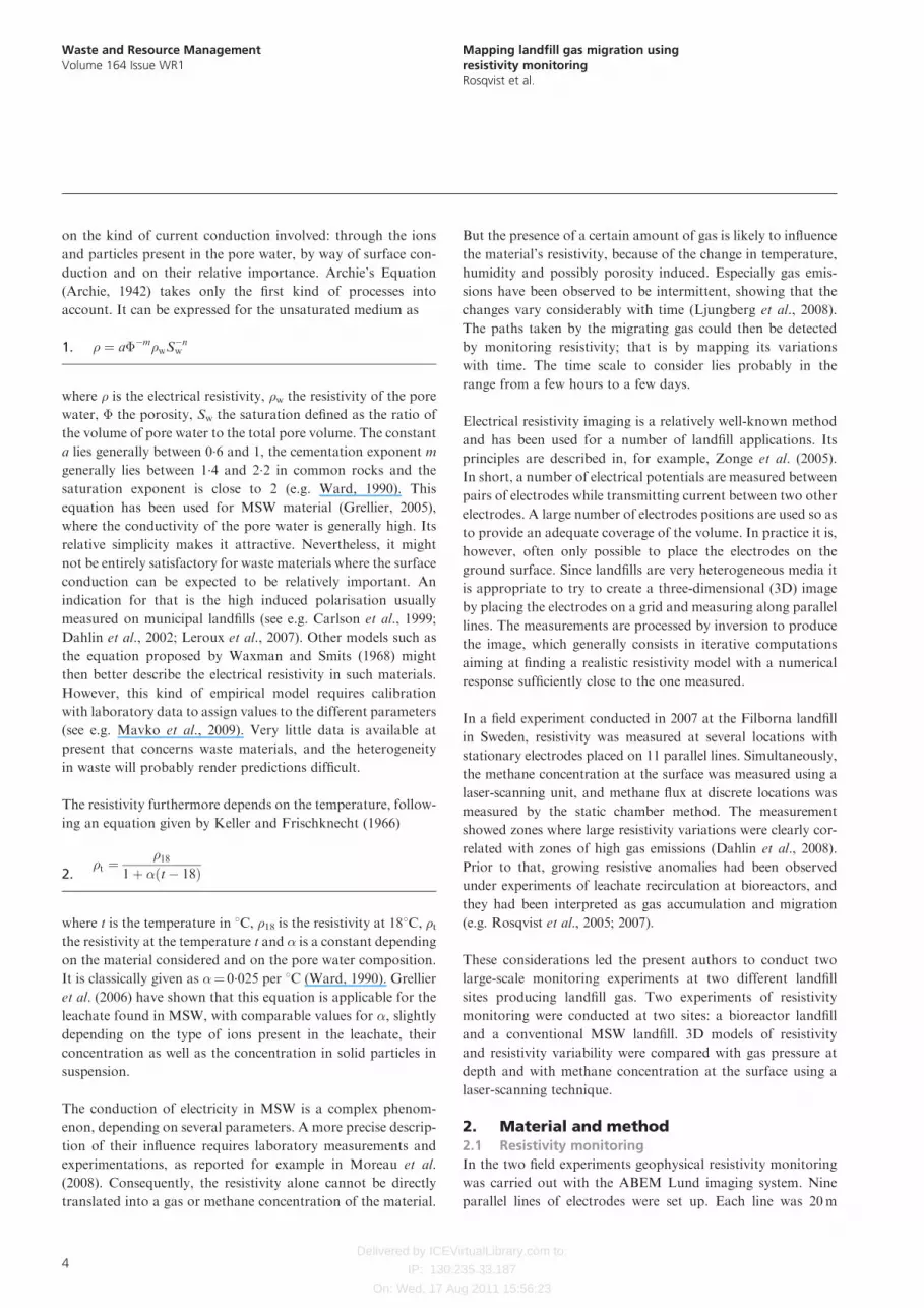
Figure 3 shows a 3D model of the resistivity for one measure-

ment conducted on 20 May 2008 at the bioreactor landfill.

The inverted resistivity was relatively low, below 10m in

large parts over the area. These low values are probably attribu-

table to the high organic content in the waste, and to the

expected high moisture and high ionic content (salinity). A

ditch filled with wooden chips where a gas-collecting pipe (see

Figure 1) was installed is clearly visible as an elongated resistive

structure, perpendicular to the resistivity lines. The same ditch

was also clearly indicated in previous investigations at the

bioreactor landfill (Rosqvist et al., 2003; 2005; 2007). The

wooden chips around the gas pipe in the ditch have a high

porosity and subsequently high gas permeability. These con-

siderations result in expectation that the ditch would be an

important path for gas migration, which to some extent could

explain the high resistivity observed.



Container Walls of compost1

0 m

2 m

4 m

6 m

8 m

21

Electrodes

Soil cover

MSW

Figure 2. General cross-section of the Filborna landfill for theinvestigated area in the direction parallel to the lines

6


IP: 130.235.33.187

On: Wed, 17 Aug 2011 15:56:23

Other highly resistive bodies are visible to the right of the ditch

on Figure 3 between about 10 cm and 2m depth. There are no

known internal structures explaining these superficial bodies.

It is suggested that the highly non-uniform structure in the

waste, for example owing to different stages of decomposition

in the waste and possibly in combination with gas migration,

contributes to these anomalies.

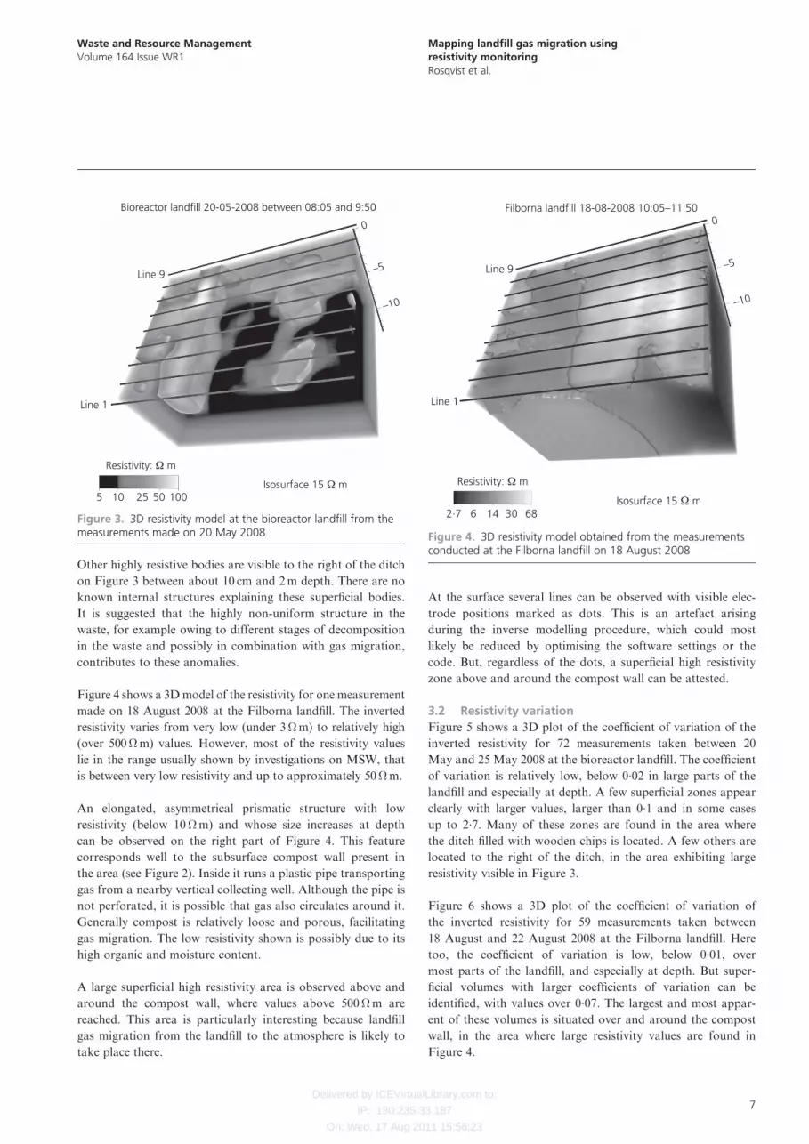
Figure 4 shows a 3Dmodel of the resistivity for one measurement

made on 18 August 2008 at the Filborna landfill. The inverted

resistivity varies from very low (under 3m) to relatively high

(over 500m) values. However, most of the resistivity values

lie in the range usually shown by investigations on MSW, that

is between very low resistivity and up to approximately 50m.

An elongated, asymmetrical prismatic structure with low

resistivity (below 10m) and whose size increases at depth

can be observed on the right part of Figure 4. This feature

corresponds well to the subsurface compost wall present in

the area (see Figure 2). Inside it runs a plastic pipe transporting

gas from a nearby vertical collecting well. Although the pipe is

not perforated, it is possible that gas also circulates around it.

Generally compost is relatively loose and porous, facilitating

gas migration. The low resistivity shown is possibly due to its

high organic and moisture content.

A large superficial high resistivity area is observed above and

around the compost wall, where values above 500m are

reached. This area is particularly interesting because landfill

gas migration from the landfill to the atmosphere is likely to

take place there.

At the surface several lines can be observed with visible elec-

trode positions marked as dots. This is an artefact arising

during the inverse modelling procedure, which could most

likely be reduced by optimising the software settings or the

code. But, regardless of the dots, a superficial high resistivity

zone above and around the compost wall can be attested.

3.2 Resistivity variation

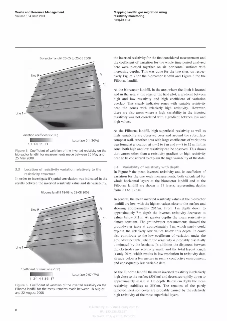
Figure 5 shows a 3D plot of the coefficient of variation of the

inverted resistivity for 72 measurements taken between 20

May and 25 May 2008 at the bioreactor landfill. The coefficient

of variation is relatively low, below 0.02 in large parts of the

landfill and especially at depth. A few superficial zones appear

clearly with larger values, larger than 0.1 and in some cases

up to 2.7. Many of these zones are found in the area where

the ditch filled with wooden chips is located. A few others are

located to the right of the ditch, in the area exhibiting large

resistivity visible in Figure 3.

Figure 6 shows a 3D plot of the coefficient of variation of

the inverted resistivity for 59 measurements taken between

18 August and 22 August 2008 at the Filborna landfill. Here

too, the coefficient of variation is low, below 0.01, over

most parts of the landfill, and especially at depth. But super-

ficial volumes with larger coefficients of variation can be

identified, with values over 0.07. The largest and most appar-

ent of these volumes is situated over and around the compost

wall, in the area where large resistivity values are found in

Figure 4.



0

–5

–10

5 10 25 50 100Isosurface 15 Ω m

Resistivity: Ω m

Bioreactor landfill 20-05-2008 between 08:05 and 9:50

Line 1

Line 9

Figure 3. 3D resistivity model at the bioreactor landfill from themeasurements made on 20 May 2008

0

–5

–10

2·7 6 14 30 68Isosurface 15 Ω m

Resistivity: Ω m

Filborna landfill 18-08-2008 10:05–11:50

Line 1

Line 9

Figure 4. 3D resistivity model obtained from the measurementsconducted at the Filborna landfill on 18 August 2008

7


IP: 130.235.33.187

On: Wed, 17 Aug 2011 15:56:23

3.3 Location of resistivity variation relatively to the

resistivity structure

In order to investigate if spatial correlation was indicated in the

results between the inverted resistivity value and its variability,

the inverted resistivity for the first considered measurement and

the coefficient of variation for the whole time period analysed

here were plotted together on six horizontal surfaces with

increasing depths. This was done for the two sites, on respec-

tively Figure 7 for the bioreactor landfill and Figure 8 for the

Filborna landfill.

At the bioreactor landfill, in the area where the ditch is located

and in the area at the edge of the field plot, a gradient between

high and low resistivity and high coefficient of variation

overlap. This clearly indicates zones with variable resistivity

near the zones with relatively high resistivity. However,

there are also areas where a high variability in the inverted

resistivity was not correlated with a gradient between low and

high values.

At the Filborna landfill, high superficial resistivity as well as

high variability are observed over and around the subsurface

compost wall. Another area with large coefficients of variations

was found at a location at x¼ 2 to 8m and y¼ 8 to 12m. In this

zone, both high and low resistivity can be observed. This shows

that causes other than a resistivity gradient or high resistivity

need to be considered to explain the high variability of the data.

3.4 Variability of resistivity with depth

In Figure 9 the mean inverted resistivity and its coefficient of

variation for the one week measurements, both calculated for

whole horizontal layers at the bioreactor landfill and at the

Filborna landfill are shown in 17 layers, representing depths

from 0.1 to 13.6m.

In general, the mean inverted resistivity values at the bioreactor

landfill are low, with the highest values close to the surface and

showing approximately 20m. From 1m depth down to

approximately 7m depth the inverted resistivity decreases to

values below 5m. At greater depths the mean resistivity is

almost constant. The groundwater measurements showed the

groundwater table at approximately 7m, which partly could

explain the relatively low values below this depth. It could

also contribute to the low coefficient of variation under the

groundwater table, where the resistivity is probably essentially

dominated by the leachate. In addition the distances between

the electrodes are relatively small, and the total layout length

is only 20m, which results in low resolution in resistivity data

already below a few metres in such a conductive environment,

and consequently less variable data.

At the Filborna landfill the mean inverted resistivity is relatively

high close to the surface (50m) and decreases rapidly down to

approximately 20m at 1m depth. Below 2m depth the mean

resistivity stabilises at 25m. The remains of the partly

removed inert soil cover are probably caused by the relatively

high resistivity of the most superficial layers.



–5

–10

1·3 3·8 11 33Isosurface 0·1 (10%)

Variation coefficient (×100)

Bioreactor landfill 20-05 to 25-05 2008

Line 1

Line 9

Figure 5. Coefficient of variation of the inverted resistivity on thebioreactor landfill for measurements made between 20 May and25 May 2008

–5

–10

1 2·1 4·1 8·3 17Isosurface 0·07 (7%)

Coefficient of variation (×100)

Filborna landfill 18-08 to 22-08 2008

Line 1

Line 9

Figure 6. Coefficient of variation of the inverted resistivity on theFilborna landfill for the measurements made between 18 Augustand 22 August 2008

8


IP: 130.235.33.187

On: Wed, 17 Aug 2011 15:56:23



2 4 6 8 10 12 14 16 18

Dis

tanc

e be

twee

n re

sist

ivity

line

s: m

Distance along resistivity lines: mLayer 2 (0·224–0·484 m)

14

12

10

8

6

4

2

2 4 6 8 10 12 14 16 18

Dis

tanc

e be

twee

n re

sist

ivity

line

s: m

Distance along resistivity lines: mLayer 1 (0–0·224 m)

14

12

10

8

6

4

2

2 4 6 8 10 12 14 16 18

Dis

tanc

e be

twee

n re

sist

ivity

line

s: m


14

12

10

8

6

4

2

2 4 6 8 10 12 14 16 18

Dis

tanc

e be

twee

n re

sist

ivity

line

s: m


14

12

10

8

6

4

2

2 4 6 8 10 12 14 16 18

Dis

tanc

e be

twee

n re

sist

ivity

line

s: m


14

12

10

8

6

4

2

2 4 6 8 10 12 14 16 18

0 10 20 50 0·2 0·5

Dis

tanc

e be

twee

n re

sist

ivity

line

s: m


Coefficient of variationof interpreted resistivityInterpreted resistivity: Ω m

14

12

10

8

6

4

2

Figure 7. Bioreactor landfill, six horizontal plans where the invertedresistivity and its variability have been plotted

9


IP: 130.235.33.187

On: Wed, 17 Aug 2011 15:56:23



2 4 6 8 10 12 14 16 18D

ista

nce

betw

een

resi

stiv

ity li

nes:

m


14

12

10

8

6

4

2

2 4 6 8 10 12 14 16 18

Dis

tanc

e be

twee

n re

sist

ivity

line

s: m

Distance along resistivity lines: mLayer 1 (0–0·224 m)

14

12

10

8

6

4

2

2 4 6 8 10 12 14 16 18

Dis

tanc

e be

twee

n re

sist

ivity

line

s: m


14

12

10

8

6

4

2

2 4 6 8 10 12 14 16 18

Dis

tanc

e be

twee

n re

sist

ivity

line

s: m


14

12

10

8

6

4

2

2 4 6 8 10 12 14 16 18

Dis

tanc

e be

twee

n re

sist

ivity

line

s: m


14

12

10

8

6

4

2

2 4 6 8 10 12 14 16 18

0 10 20 50 0·1 0·2

Dis

tanc

e be

twee

n re

sist

ivity

line

s: m


Coefficient of variationof interpreted resistivityInterpreted resistivity: Ω m

14

12

10

8

6

4

2

Figure 8. Filborna landfill: six horizontal plans where the invertedresistivity and its variability have been plotted

10


IP: 130.235.33.187

On: Wed, 17 Aug 2011 15:56:23

At the bioreactor landfill the uppermost layers show relatively

high coefficients of variation with a peak at layer 4, which

is found at approximately 1m depth. Under this depth the

coefficient of variation decreases down to approximately 0.2

at about 5m depth. At greater depths the coefficient of variation

remains low, about 0.2, and constant.

The coefficient of variation at the Filborna landfill shows a

similar pattern with large values (over 3) in the most super-

ficial layers and much lower and relatively stable values at

depths below 2m (0.7 to 0.6). A peak appears here also

between 1 and 2m depth with values rising to approximately

1 to 1.5.



0

10

20

30

40

50

60

0

0·5

1·0

1·5

2·0

2·5

3·0

3·5

4·0

0

10

20

30

40

50

60

0 1 2 3 4 5 6 7 8 9 10 11 12 13 14 15Depth: m

(a)

0 1 2 3 4 5 6 7 8 9 10 11 12 13 14 15Depth: m

(b)

Mea

n re

sist

ivity

: Ω m

Mea

n re

sist

ivity

: Ω m

0

0·5

1·0

1·5

2·0

2·5

3·0

3·5

Coe

ffic

ient

of

varia

tion

Coe

ffic

ient

of

varia

tion

Mean resistivityCoefficient of variation

Mean resistivityCoefficient of variation

Figure 9. Mean resistivity and coefficient of variation at differentdepths at the (a) bioreactor and (b) Filborna landfills (calculated forall cells in a layer)

11


IP: 130.235.33.187

On: Wed, 17 Aug 2011 15:56:23

3.5 Methane emissions at the surface

On Figure 10 laser-scanning results at the Filborna landfill show

high levels of methane emissions (between 200 and 600 ppm/m)

at the surface along the subsurface compost wall. An area with

emissions at lower levels (between 70 and 100 ppm/m) is also

found over the monitored area. This figure summarises the

outcome of several measurements over a few days. The loca-

tions of higher methane concentrations were stable, but the

concentrations were variable. Their range is therefore given,

instead of mean values, in order to express this variability.

The high levels of methane emissions along the compost wall

are particularly interesting since they coincide well with the

high inverted resistivity values and their high variability found

in this zone (Figures 4, 6 and 8). The localisation of methane

emissions correlates well with the localisation of inverted

resistivity variations, showing that the latter can be interpreted

as an indication of methane leakage along the compost wall.

3.6 Pore pressure monitoring

Figure 11 shows a negative pore pressure of approximately 1m

H2O for sensor B1 in the bioreactor landfill, possibly explained

by the gas outtake by way of the closely situated gas collection

pipe. Initially the sensor B2 registered a pressure of 3m H2O,

but then gradually decreased to a rather stable value of 1.5m

H2O after a month. The decreasing pore pressure could be

explained by a gas leakage through the bentonite sealing

surrounding the Bat sensor pipe or a generally decreasing gas

pressure at this location.

In Figure 12 the sensor F1 placed in a high resistive area at

Filborna landfill shows a high pore pressure, initially at a

maximum value of 7m H2O. During the monitored period the

recorded value decreases gradually, similarly to what happens

for sensor B2 on the bioreactor. After 12 days the pore pressure

was 3.5m H2O on this location. This decrease could, as for the

sensor B2, be explained either by a gas leakage through the

bentonite sealing surrounding the Bat sensor or by a generally



Container

Emissions70–100 ppm/m

Emissions200–6000 ppm/m

Line 121

19

17

15

13

11

9

75

3

1

Line 2Line 3

Line 4Line 5

Line 6Line 7

Line 8Line 9

Figure 10. Methane concentration at the surface above Filbornalandfill obtained with laser scanning between 18 August and22 August 2008

Time: days

05-06-200812:00

12-06-200812:00

19-06-200812:00

BAT sensor B2

BAT sensor B1

Pore

pre

ssur

e (m

H2O

)

4

3

2

1

0

–1

–2

Figure 11. Pore pressure measurements on the bioreactor landfillbetween 19 May and 24 July 2008

Time: days

29-08-200816:00

BAT sensor F2

BAT sensor F1

Pore

pre

ssur

e (m

H2O

)

8

7

6

5

4

3

2

1

0

–1

Figure 12. Pore pressure measurements on the Filborna landfillbetween 22 August and 3 September 2008

12


IP: 130.235.33.187

On: Wed, 17 Aug 2011 15:56:23

decreasing pore pressure in the area. The sensor F2 was placed

in a low resistive area. The measured pore pressure stayed stable

and close to 0m H2O under the whole monitored period. This

correlates well with the low resistivity and low variability

assumed as indicating low gas activity.

At both sites the groundwater level was below the depth of the

sensors and, therefore, the most plausible explanation of the

large positive pore pressure values on sensors B2 and F1

particularly is the presence of landfill gas.

4. Discussion and conclusionsIn this study the main focus was on the temporal and spatial

variation of the inverted resistivity, since it was assumed that

variability, in particular temporal variability, could indicate

gas migration.

The results of the resistivity measurements were regarded as con-

sistent since the resistivity values found lie in the same range as in

previous investigations at MSW landfills, some of them also

made on the bioreactor landfill. Large variations in the inter-

preted resistivity coinciding with large interpreted resistivity

values have been found at several areas on the two monitored

sites, a bioreactor landfill and an ordinary MSW landfill. A

large range of materials with very different resistivity can be

assumed in the landfills. Yet the resistivity structure was consis-

tent with the known existing structures inside both sites, that is,

a trench filled with wooden chips in the bioreactor landfill and

a compost wall in the Filborna landfill. These structures can

also be expected to constitute important migration paths for

the landfill gas, since they have a relatively high porosity and in

the bioreactor landfill the ditch contains a pipe for landfill gas

collection. Thus, the results of the study confirm that resistivity

remains a powerful tool for detecting internal features in landfills.

At the Filborna landfill the resistivity values were most variable

in delimited superficial areas over the subsurface compost wall.

In this area also high methane concentration was measured in

the air using the laser-scanning instrument. This strengthens

the interpretation of the high variability in the interpreted

resistivity being an indicator of landfill gas migration. In fact,

the clear correlation between subsurface measurements by

means of resistivity and the laser-scanning results above the

surface is regarded as the most interesting result in this study.

The successive time steps were inverted separately without any

constraints between successive models that could focus the

inversion on the changes. This could possibly result in artefacts,

but this effect was minimised by the use of the same geometry

and parameters all along, as well as a low number of iterations.

Time-lapse procedures are generally preferable, but the choice

of the reference model can be difficult. In the study presented

here, the amplitude of the observed variations and the

consistency of their pattern support the interpretation of them

being caused by actual physical changes inside the landfill.

The resistivity variations were found to be more pronounced at

the superficial zones and they decreased generally with depth, to

reach small values below a few metres. One explanation is the

limited depth of investigation owing to the experimental set-

up; that is, with relatively small distances, over an overall con-

ductive landfill mass. Consequently, only limited information

could be achieved about the resistivity at depth. An illustration

of this general limitation is given in Jolly et al. (2007), with com-

puted examples. A complementary explanation is the expected

large temporal variations close to the ground surface, most

sensitive to variable atmospheric influence. As a result of gas

migration from greater depths, it can be assumed that the

landfill gas content is higher close to the surface. However, it

should be pointed out that deeper structures containing large

amounts of landfill gas most likely exist.

It has been shown that it is possible to detect gas accumulation

and leakage at the surface but it would also be desirable to

localise where the gas forms as well as its migration paths.

Since the results demonstrate that superficial areas with higher

gas pressure and/or migration can be localised, zones at greater

depths containing significant amounts of gas may be found,

provided that appropriate geometrical configuration is used in

the resistivity monitoring. It is therefore suggested that future

investigations should aim at detailed measurements at greater

depth using this technique.

The use of geophysical resistivity monitoring for imaging paths

of gas migration at landfills is promising, even if the internal

process in the waste mass is complicated and the variation of

resistivity is attributable to several intricate factors. The

resistivity technique has reached such a state that it is possible

to use in real-case applications to reasonable costs. When

monitoring, the only part of the equipment that must stay in

place is the electrodes, and they constitute the cheapest and

least vulnerable part. Since the gas emissions and the resistivity

variations happen relatively quickly and irregularly in time, it

is important to measure resistivity over time. Simple field

procedures, involving less measurement, could give good results

in practice at lower costs. An example of such a field survey is

given in Dahlin et al. (2008).

More accurate knowledge about the dependence of resistivity

variation to temperature, porosity, organic content and moisture

content inMSWmaterials would contribute to a safer interpreta-

tion of the results. It has been noted in studies concerning the

dependence of resistivity to the salinity of the pore water (e.g.

Taylor and Barker, 2002 in sandstones) and in studies concerning

its dependence to the temperature (e.g. Aaltonen, 2001 in soils) as

well as in studies concerning its dependence to moisture (e.g.



13


IP: 130.235.33.187

On: Wed, 17 Aug 2011 15:56:23

Moreau et al., 2008 in waste) that it could vary depending on the

nature of material considered and on its internal structure. There-

fore general laws based on extensive laboratory measurements on

different samples of MSW materials could be extremely useful.

The dependence of resistivity to the above-named parameters in

MSW has still only been partially investigated.

Since the resistivity in waste depends on several interacting

parameters, it would be useful to measure at least one of them

when monitoring, for instance the temperature. It is relatively

easy to do this on the ground surface, but installing sensors at

depth can be complicated and costly.

Furthermore, for future investigations it is essential to collect all

available information about the landfill in question, such as:

its construction, its age, the deposited waste, properties of the

leachate, possible watering pipes, the gas extraction system

and information about gas leakages. This kind of information

is important to ensure high quality in the interpretation of the

resistivity results.

With the aim of a better understanding of the gas processes in

MSW landfills, it is concluded that the techniques described

here can be used and improved by future research and develop-

ment focused on studies at different scales, and on the

interaction between different processes.

AcknowledgementsThe Swedish Waste Management, the Swedish Gas Centre,

Sven Tyrens Stiftelse, NSR AB, Narab and Vafab are

acknowledged for the financial support of the study.

REFERENCES

Aaltonen J (2001) Seasonal resistivity variations in some

different Swedish soils. European Journal of Environmental

and Engineering Geophysics 6: 33–45.

Archie GE (1942) The electrical resistivity log as an aid to

determine some reservoir characteristics. Transactions of

American Institute of Mineral, Metal and Petroleum

Engineering 146: 389–409.

Carlson NR, Mayerle CM and Zonge KL (1999) Extremely fast

IP used to delineate buried landfills. Proceedings of the 5th

Meeting of the EEGS – European Section, Budapest,

September 6–9.

Dahlin T, Leroux V and Nissen J (2002) Measuring techniques

in induced polarisation imaging. Journal of Applied

Geophysics 50(3): 279–298.

Dahlin T, Leroux V, Rosqvist H et al. (2008) Potential of

geoelectrical imaging techniques for detecting subsurface

gas migration in landfills – an experiment. Proceedings of

14th European Meeting of Environmental and Engineering

Geophysics, Near Surface Conference, Krakow, September

15–17, B05, 4pp.

Grellier S (2005) Suivi Hydrologique des Centres de Stockage

de Dechet-bioreacteurs par Measures Geophysiques. PhD

thesis, Universite Paris 6, France, in French.

Grellier S, Robain H, Bellier G and Skhiri N (2006) Influence

of temperature on the electrical conductivity of leachate

from municipal solid waste. Journal of Hazardous Materials

137(1): 612–617.

Johansson S (2009) Electrical Resistivity as a Tool for

Analyzing Soil Gas Movements and Gas Emissions from

Landfill soils. MS Thesis, Department of Physics, Lund

University, Sweden.

Jolly J, Barker R, Beaven R and Herbert A (2007) Time-lapse

electrical imaging to study fluid movement within a landfill.

Proceedings of Sardinia-07, 11th International Waste

Management and Landfill Symposium, Cagliari.

Keller GV and Frischknecht FC (1966) Electrical Methods in

Geophysical Prospecting. Pergamon Press, Oxford.

Leroux V, Dahlin T and Svensson M (2007) Dense resistivity

and IP profiling for a landfill restoration project at Harlov,

Southern Sweden. Waste Management and Research 25(1):

49–60.

Ljungberg S-A, Meijer J-E, Rosqvist H and Martensson S-G

(2008) Detection and Quantification of Methane Leakage

from Landfills. Svenskt Gastekniskt Center, ISRN SGC-R-

204-SE, Report SGC 204. See www.sgc.se.

Loke MH (2008) Manual for Res3DInv. See

www.geoelectrical.com.

Loke MH and Barker R (1996) Practical techniques for 3D

resistivity surveys and data inversion. Geophysical

Prospecting 44(3): 499–523.

Loke MH, Acworth I and Dahlin T (2003) A comparison of

smooth and blocky inversion methods in 2-D electrical

imaging surveys. Exploration Geophysics 34(3): 182–187.

Mavko G, Mukerji T and Dvorkin J (2009) The Rock Physics

Handbook: Tool for Seismic Analysis of Porous Media.

Cambridge University Press.

Moreau S, Bouye J-F, Saidi F and Ripaud F (2008) Towards

the determination of volumetric water content in waste

body from electrical resistivity: laboratory tests part II.

Workshop on Geophysical Measurements at Landfills,

Tyrens org, Malmo, Sweden.

O’Leary P and Walsh P (2002) Landfill gas movement, control

and energy recovery. Waste Age, January, pp. 48–53.

Rosqvist H, Dahlin T, Fourie A. et al. (2003) Mapping of

leachate plumes at two landfill sites in South Africa using

geoelectrical imaging techniques. Proceedings of 9th

International Waste Management and Landfill Symposium,

Cagliari.

Rosqvist H, Dahlin T and Lindhe C (2005) Investigation of

water flow in a bioreactor landfill using geoelectrical

imaging techniques. Proceedings of Sardinia-05, 10th

International Waste Management and Landfill Symposium,

Cagliari.



14


IP: 130.235.33.187

On: Wed, 17 Aug 2011 15:56:23

Rosqvist H, Dahlin T, Linders F and Meijer J-E (2007)

Detection of water and gas migration in a bioreactor

landfill using geoelectrical imaging and a tracer test.

Proceedings Sardinia-07, 11th International Waste

Management and Landfill Symposium, Cagliari, Sardinia,

Italy.

Taylor S and Barker R (2002) Resistivity of partially saturated

Triassic sandstone. Geophysical Prospecting 50(6): 603–613.

Torstensson B-A (1984) A new system for groundwater

monitoring. Ground Water Monitoring & Remediation 4(4):

131–138.

Ward S (1990) Resistivity and induced polarization methods.

In Investigations in Geophysics No 5: Geotechnical and

Environmental Geophysics, vol. I: Review and Tutorial.

Society of Exploration Geophysicists, Tulsa, pp. 147–189.

Waxman MH and Smits LJM (1968) Electrical conduction in

oil-bearing Shaly sands. Society of Petroleum Engineers

Journal 8(2): 107–122.

Zonge K, Wynn J and Urquhart S (2005) Resistivity, induced

polarisation and complex resistivity in near-surface

geophysics. SEG Investigations in Geophysics Series 13:

265–300.

WHAT DO YOU THINK?

To discuss this paper, please email up to 500 words to the

editor at [email protected]. Your contribution will be

forwarded to the author(s) for a reply and, if considered

appropriate by the editorial panel, will be published as a

discussion in a future issue of the journal.

Proceedings journals rely entirely on contributions sent in

by civil engineering professionals, academics and students.

Papers should be 2000–5000 words long (briefing papers

should be 1000–2000 words long), with adequate illustra-

tions and references. You can submit your paper online

via www.icevirtuallibrary.com/content/journals, where you



15