ISSN 1069�3513, Izvestiya, Physics of the Solid Earth, 2012, Vol. 48, No. 1, pp. 42–60. © Pleiades Publishing, Ltd., 2012.Original Russian Text © D.M. Pechersky, A.A. Lyubushin, Z.V. Sharonova, 2012, published in Fizika Zemli, 2012, No. 1, pp. 44–62.

42

INTRODUCTION

In this work, we compare four types of processes:(1) those occurring exceptionally in the core of theEarth (variations and reversals of the geomagneticfield); (2) those originating at the core�mantle bound�ary, rising upwards, and reaching the surface of theEarth (the plumes); (3) those strictly confined to theEarth’s surface (the changes in the organics); and(4) those synchronously involving the whole body of theplanet (the Earth’s rotation around its axis). Previously,we revealed the increase in the amplitude of directionalgeomagnetic variations on approaching the centers ofthe world magnetic anomalies and epicenters of themantle plumes (Pechersky, 2001; 2007; 2009; Pecherskyand Garbuzenko, 2005). This fact points to tight cou�pling between these factors, as all of them are generatedby local disturbances at the core–mantle boundary(Grachev, 2000; Zharkov, Karpov, and Leont’ev, 1984;Ernst and Buchan, 2003, etc.).

When comparing geomagnetic reversals against asuccession of stratigraphic stages, it was found that thestratigraphic boundaries do not correlate to the reversalswhile the rate of flips in geomagnetic polarity is syn�chronized with the rate of changes of stratigraphicstages (Pechersky, 2000; Pechersky, Lyubushin, andSharonova, 2010). This feature is only recognizablewith extensive averaging of the data over a period of10 m.y., as the durations of magnetochrons (the timegap between the adjacent reversals) and the stages aresubstantially different: the modal duration of a magne�tochron is 0.4 m.y. against the 4 m.y. modal duration ofa stage. It is quite reasonable then to seek a correlationbetween the units which have more similar durations,

such as magnetochrons and biozones. The key difficultyin this work lies in the fact that, in contrast to the scaleof stages, no common geochronological stratification issuggested for the biozones. Without intending todevelop such a scale, we attempt to construct somecompilation of the data on the common boundaries ofthe biozones for correlating them to the geomagneticreversals. This correlation is carried out in the presentpaper.

THE METHODS OF COLLECTINGAND ANALYZING THE DATA

The time distributions of geomagnetic reversals wereanalyzed using the magnetochronostratigraphic scalefor the Phanerozoic (Table 1) based on the collection ofdata presented in (Guzhikov, 2004; Molostovskii, Pech�ersky, and Frolov, 2007; Pechersky, Lyubushin, andSharonova, 2010; Khramov and Shkatova, 2000; Pavlovand Gallet, 2005). The changes in the organics aretraced against the alteration of biozones. The latter arethe shortest stratigraphic units that have an almost glo�bal extension. In contrast to the geochronology of stagesfor which the global scale has been developed, there isno common global geochronological stratification forbiozones. This is, obviously, applicable to yet shorterstratigraphic units such as subzones and horizons.

These units have a regional or local extent; thus, it ispractically impossible to compile a global scheme forthe changes of the subzones. Both magnetostratigraphicand biostratigraphic data contain plenty of controversialage estimates for the boundaries between stages, mag�netochrons, and other units, which are given different

On the Coherence between Changes in Biotaand Geomagnetic Reversals in the Phanerozoic

D. M. Pechersky, A. A. Lyubushin, and Z. V. SharonovaInstitute of Physics of the Earth, Russian Academy of Sciences, ul. Bol’shaya Gruzinskaya 10, Moscow, 123995 Russia

Received May 5, 2010; in final form, August 2, 2010

Abstract—The data on geomagnetic reversals, organic changes, and lower�mantle plume magmatism in thePhanerozoic are collected and correlated. No direct relationship is revealed between the geomagnetic rever�sals, plumes, and biozones. However, the frequency of geomagnetic reversals is found to correlate to the fre�quency of biozonal alterations. We relate this inconsistency to the coupling of the two processes, which aremutually independent, with the long�term changes in the Earth’s rotation. The plumes are formed at thecore�mantle boundary and, thus, the reversals should have a different source. We hypothesize that the changein the geomagnetic polarity is due to the nonuniform rotation of the inner core relative to the mantle in com�bination with the changes in the axial tilt of the Earth’s rotation.

Keywords: geomagnetic reversal, magnetochron, inner core of the Earth, biozone, biota, the Phanerozoic.

DOI: 10.1134/S1069351311120081

IZVESTIYA, PHYSICS OF THE SOLID EARTH Vol. 48 No. 1 2012

ON THE COHERENCE BETWEEN CHANGES IN BIOTA 43

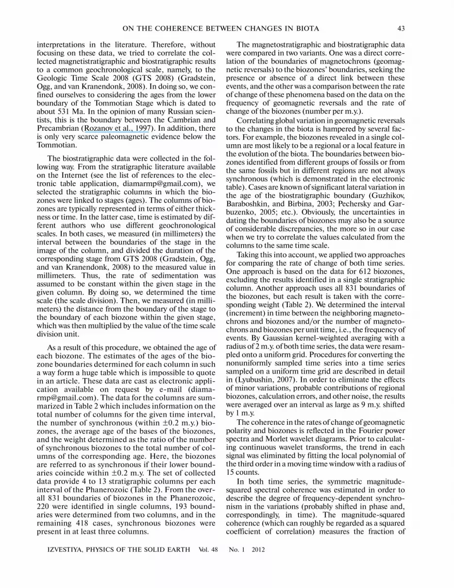
interpretations in the literature. Therefore, withoutfocusing on these data, we tried to correlate the col�lected magnetistratigraphic and biostratigraphic resultsto a common geochronological scale, namely, to theGeologic Time Scale 2008 (GTS 2008) (Gradstein,Ogg, and van Kranendonk, 2008). In doing so, we con�fined ourselves to considering the ages from the lowerboundary of the Tommotian Stage which is dated toabout 531 Ma. In the opinion of many Russian scien�tists, this is the boundary between the Cambrian andPrecambrian (Rozanov et al., 1997). In addition, thereis only very scarce paleomagnetic evidence below theTommotian.

The biostratigraphic data were collected in the fol�lowing way. From the stratigraphic literature availableon the Internet (see the list of references to the elec�tronic table application, diamarmp@gmail.com), weselected the stratigraphic columns in which the bio�zones were linked to stages (ages). The columns of bio�zones are typically represented in terms of either thick�ness or time. In the latter case, time is estimated by dif�ferent authors who use different geochronologicalscales. In both cases, we measured (in millimeters) theinterval between the boundaries of the stage in theimage of the column, and divided the duration of thecorresponding stage from GTS 2008 (Gradstein, Ogg,and van Kranendonk, 2008) to the measured value inmillimeters. Thus, the rate of sedimentation wasassumed to be constant within the given stage in thegiven column. By doing so, we determined the timescale (the scale division). Then, we measured (in milli�meters) the distance from the boundary of the stage tothe boundary of each biozone within the given stage,which was then multiplied by the value of the time scaledivision unit.

As a result of this procedure, we obtained the age ofeach biozone. The estimates of the ages of the bio�zone boundaries determined for each column in sucha way form a huge table which is impossible to quotein an article. These data are cast as electronic appli�cation available on request by e�mail (diama�rmp@gmail.com). The data for the columns are sum�marized in Table 2 which includes information on thetotal number of columns for the given time interval,the number of synchronous (within ±0.2 m.y.) bio�zones, the average age of the bases of the biozones,and the weight determined as the ratio of the numberof synchronous biozones to the total number of col�umns of the corresponding age. Here, the biozonesare referred to as synchronous if their lower bound�aries coincide within ±0.2 m.y. The set of collecteddata provide 4 to 13 stratigraphic columns per eachinterval of the Phanerozoic (Table 2). From the over�all 831 boundaries of biozones in the Phanerozoic,220 were identified in single columns, 193 bound�aries were determined from two columns, and in theremaining 418 cases, synchronous biozones werepresent in at least three columns.

The magnetostratigraphic and biostratigraphic datawere compared in two variants. One was a direct corre�lation of the boundaries of magnetochrons (geomag�netic reversals) to the biozones’ boundaries, seeking thepresence or absence of a direct link between theseevents, and the other was a comparison between the rateof change of these phenomena based on the data on thefrequency of geomagnetic reversals and the rate ofchange of the biozones (number per m.y.).

Correlating global variation in geomagnetic reversalsto the changes in the biota is hampered by several fac�tors. For example, the biozones revealed in a single col�umn are most likely to be a regional or a local feature inthe evolution of the biota. The boundaries between bio�zones identified from different groups of fossils or fromthe same fossils but in different regions are not alwayssynchronous (which is demonstrated in the electronictable). Cases are known of significant lateral variation inthe age of the biostratigraphic boundary (Guzhikov,Baraboshkin, and Birbina, 2003; Pechersky and Gar�buzenko, 2005; etc.). Obviously, the uncertainties indating the boundaries of biozones may also be a sourceof considerable discrepancies, the more so in our casewhen we try to correlate the values calculated from thecolumns to the same time scale.

Taking this into account, we applied two approachesfor comparing the rate of change of both time series.One approach is based on the data for 612 biozones,excluding the results identified in a single stratigraphiccolumn. Another approach uses all 831 boundaries ofthe biozones, but each result is taken with the corre�sponding weight (Table 2). We determined the interval(increment) in time between the neighboring magneto�chrons and biozones and/or the number of magneto�chrons and biozones per unit time, i.e., the frequency ofevents. By Gaussian kernel�weighted averaging with aradius of 2 m.y. of both time series, the data were resam�pled onto a uniform grid. Procedures for converting thenonuniformly sampled time series into a time seriessampled on a uniform time grid are described in detailin (Lyubushin, 2007). In order to eliminate the effectsof minor variations, probable contributions of regionalbiozones, calculation errors, and other noise, the resultswere averaged over an interval as large as 9 m.y. shiftedby 1 m.y.

The coherence in the rates of change of geomagneticpolarity and biozones is reflected in the Fourier powerspectra and Morlet wavelet diagrams. Prior to calculat�ing continuous wavelet transforms, the trend in eachsignal was eliminated by fitting the local polynomial ofthe third order in a moving time window with a radius of15 counts.

In both time series, the symmetric magnitude�squared spectral coherence was estimated in order todescribe the degree of frequency�dependent synchro�nism in the variations (probably shifted in phase and,correspondingly, in time). The magnitude�squaredcoherence (which can roughly be regarded as a squaredcoefficient of correlation) measures the fraction of

44

IZVESTIYA, PHYSICS OF THE SOLID EARTH Vol. 48 No. 1 2012

PECHERSKY et al.

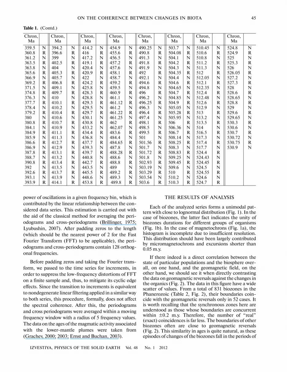
Table 1. The scale of geomagnetic reversals in the Phanerozoic

Chron, Ma

Chron, Ma

Chron, Ma

Chron, Ma

Chron, Ma

Chron, Ma

Chron, Ma

Chron, Ma

0.78 N 11.71 R 25.45 N 50.03 R 128.1 N 151.5 R 177.9 N 260.5 R0.91 R 11.9 N 25.84 R 50.66 N 128.13 R 151.6 N 178.7 R 260.7 N0.97 N 12.05 R 26.01 N 51.85 R 128.2 N 152.2 R 180.4 N 261 R1.65 R 12.34 N 26.29 R 52.08 N 128.65 R 152.4 N 182.4 R 261.5 N1.88 N 12.68 R 26.37 N 52.13 R 128.9 N 152.8 R 185.6 N 262 R2.06 R 12.71 N 26.44 R 52.83 N 129.1 R 152.9 N 186.3 R 263 N2.09 N 12.79 R 27.13 N 53.15 R 129.2 N 153.1 R 188.9 N 263.5 R2.45 R 12.84 N 27.52 R 53.2 N 129.7 R 153.2 N 199.3 R 264 N2.91 N 13.04 R 28.07 N 53.39 R 129.95 N 153.5 R 202.3 N 264.6 R2.98 R 13.21 N 28.12 R 53.69 N 130.8 R 153.8 N 203 R 264.8 N3.07 N 13.4 R 28.51 N 54.05 R 130.95 N 154 R 214.2 N 265 R3.17 R 13.64 N 29 R 54.65 N 131.1 R 154.3 N 214.9 R 265.4 N3.4 N 13.87 R 29.29 N 57.19 R 131.3 N 154.7 R 216.5 N 279.5 R3.87 R 14.24 N 29.35 R 57.8 N 131.8 R 155.08 N 217.9 R 280.5 N3.99 N 14.35 R 29.58 N 58.78 R 132.3 N 155.1 R 219.1 N 305.1 R4.12 R 14.79 N 30.42 R 59.33 N 133.4 R 155.2 N 220.4 R 305.6 N4.26 N 14.98 R 30.77 N 61.65 R 133.95 N 155.4 R 221 N 307.4 R4.41 R 15.07 N 30.82 R 62.17 N 134.21 R 155.6 N 222.7 R 308.2 N4.48 N 15.23 R 31.21 N 62.94 R 134.3 N 155.8 R 224.2 N 311.5 R4.79 R 15.35 N 31.6 R 63.78 N 135.2 R 156.05 N 225.8 R 312.2 N5.08 N 16.27 R 32.01 N 64.16 R 135.25 N 156.1 R 236 N 315.1 R5.69 R 16.55 N 34.26 R 64.85 N 135.6 R 156.29 N 241.3 R 315.3 N5.96 N 16.59 R 34.44 N 65.7 R 135.8 N 156.4 R 242.9 N 315.8 R6.04 R 16.75 N 34.5 R 68.1 N 136.05 R 156.7 N 243.4 R 316.8 N6.33 N 16.82 R 34.82 N 68.3 R 136.2 N 156.8 R 244 N 317.3 R6.66 R 16.99 N 36.12 R 69.6 N 136.7 R 156.96 N 245 R 317.7 N6.79 N 17.55 R 36.32 N 72.6 R 136.9 N 157.1 R 247 N 318.3 R7.01 R 17.84 N 36.35 R 73.1 N 137.8 R 157.2 N 247.4 R 320 N7.1 N 18.07 R 36.54 N 73.2 R 138.3 N 157.3 R 248.9 N 321 R7.17 R 18.09 N 36.93 R 74.4 N 139.4 R 157.6 N 249.7 R 321.5 N7.56 N 18.5 R 37.16 N 74.8 R 140.8 N 157.85 R 249.9 N 321.8 R7.62 R 19 N 37.31 R 74.85 N 141.8 R 158.37 N 250.1 R 321.9 N7.66 N 19.26 R 37.58 N 75.2 R 142.05 N 160.3 R 250.2 N 322.6 R8.02 R 20.23 N 37.63 R 79.8 N 143.6 R 160.8 N 250.8 R 323.3 N8.29 N 20.52 R 38.01 N 81.6 R 143.7 N 161.2 R 251 N 323.9 R8.4 R 20.74 N 38.28 R 82.2 N 144.4 R 161.4 N 251.2 R 324.6 N8.54 N 20.97 R 39.13 N 83.2 R 144.5 N 161.6 R 252 N 325.6 R8.78 R 21.37 N 39.2 R 88.3 N 144.7 R 161.7 N 253.5 R 326.7 N8.83 N 21.6 R 39.39 N 88.7 R 145.3 N 162.2 R 254 N 330.7 R8.91 R 21.75 N 39.45 R 107.1 N 145.8 R 162.3 N 254.5 R 331.6 N9.09 N 21.93 R 39.77 N 108.1 R 146.1 N 162.7 R 254.7 N 332.4 R9.14 R 22.03 N 39.94 R 109.1 N 146.2 R 164.1 N 254.9 R 333.2 N9.48 N 22.23 R 40.36 N 110.2 R 146.6 N 164.7 R 255 N 333.6 R9.49 R 22.6 N 40.43 R 116.1 N 147.4 R 165.3 N 255.2 R 333.9 N9.8 N 22.9 R 40.83 N 116.3 R 147.8 N 166.6 R 255.5 N 334.2 R9.83 R 23.05 N 40.9 R 119.7 N 149.2 R 167.7 N 256 R 335 N

10.13 N 23.25 R 41.31 N 120.7 R 149.8 N 168.8 R 256.5 N 335.3 R10.15 R 23.38 N 42.14 R 123.6 N 149.95 R 169.2 N 257 R 335.9 N10.43 N 24.62 R 42.57 N 124.2 R 150.05 N 169.7 R 257.5 N 338.9 R10.57 R 24.77 N 43.13 R 124.8 N 150.7 R 171 N 258 R 344 N10.63 N 25.01 R 44.57 N 126.8 R 150.8 N 171.7 R 258.5 N 345.9 R11.11 R 25.11 N 47.01 R 127.5 N 151 R 172.8 N 259.5 R 347 N11.18 N 25.17 R 48.51 N 128.05 R 151.3 N 176 R 260 N 356 R

IZVESTIYA, PHYSICS OF THE SOLID EARTH Vol. 48 No. 1 2012

ON THE COHERENCE BETWEEN CHANGES IN BIOTA 45

power of oscillations in a given frequency bin, which iscontributed by the linear relationship between the con�sidered data series. This estimation is carried out withthe aid of the classical method for averaging the peri�odograms and cross�periodograms (Brillinger, 1975;Lyubushin, 2007). After padding zeros to the length(which should be the nearest power of 2 for the FastFourier Transform (FFT) to be applicable), the peri�odograms and cross�periodograms contain 128 orthog�onal frequencies.

Before padding zeros and taking the Fourier trans�form, we passed to the time series for increments, inorder to suppress the low�frequency distortions of FFTon a finite sample and, thus, to mitigate its cyclic edgeeffects. Since the transition to increments is equivalentto nondegenerate linear filtering applied in a similar wayto both series, this procedure, formally, does not affectthe spectral coherence. After this, the periodogramsand cross periodograms were averaged within a movingfrequency window with a radius of 5 frequency values.The data on the ages of the magmatic activity associatedwith the lower�mantle plumes were taken from(Grachev, 2000; 2003; Ernst and Buchan, 2003).

THE RESULTS OF ANALYSIS

Each of the analyzed series forms a unimodal pat�tern with close to lognormal distribution (Fig. 1). In thecase of biozones, the latter fact indicates the unity ofbiozones durations for different groups of organisms(Fig. 1b). In the case of magnetochrons (Fig. 1a), thehistogram is incomplete due to insufficient resolution.This distribution should have been largely contributedby micromagnetochrons and excursions shorter than0.05 m.y.

If there indeed is a direct correlation between thestate of particular populations and the biosphere over�all, on one hand, and the geomagnetic field, on theother hand, we should see it when directly contrastingthe data on geomagnetic reversals against the changes inthe organics (Fig. 2). The data in this figure have a widescatter of values. From a total of 831 biozones in thePhanerozoic (Table 2, Fig. 2), their boundaries coin�cide with the geomagnetic reversals only in 52 cases. Itis worth recalling that the synchronous zones here areunderstood as those whose boundaries are concurrentwithin ±0.2 m.y. Therefore, the number of “real”(exact) coincidences is far less. The boundaries of otherbiozones often are close to geomagnetic reversals(Fig. 2). This similarity in ages is quite natural, as theseepisodes of changes of the biozones fall in the periods of

Table 1. (Contd.)

Chron, Ma

Chron, Ma

Chron, Ma

Chron, Ma

Chron, Ma

Chron, Ma

Chron, Ma

Chron, Ma

359.5 N 394.2 N 414.2 N 454.9 N 490.25 N 503.7 N 510.45 N 524.8 N360.8 R 396.6 R 416 R 455.6 R 490.8 R 504.08 R 510.6 R 524.9 R361.2 N 399 N 417.2 N 456.5 N 491.3 N 504.1 N 510.8 N 525 N363.5 R 402.5 R 419.1 R 457.2 R 491.8 R 504.2 R 511.2 R 525.3 R363.8 N 404 N 420.4 N 457.6 N 491.9 N 504.3 N 511.3 N 526 N365.6 R 405.3 R 420.9 R 458.1 R 492 R 504.35 R 512 R 526.05 R366.9 N 405.7 N 422 N 458.7 N 492.1 N 504.4 N 512.05 N 527.2 N369.2 R 406.8 R 424.2 R 459.2 R 494.6 R 504.6 R 512.1 R 527.3 R371.5 N 409.1 N 425.8 N 459.5 N 494.8 N 504.65 N 512.35 N 528 N374.8 R 409.7 R 428.3 R 460.9 R 496 R 504.7 R 512.4 R 528.6 R376.3 N 410 N 428.8 N 461.1 N 496.2 N 504.85 N 512.48 N 528.65 N377.7 R 410.1 R 429.3 R 461.12 R 496.25 R 504.9 R 512.6 R 528.8 R378.4 N 410.2 N 429.5 N 461.2 N 496.3 N 505.05 N 512.9 N 529 N379.2 R 410.4 R 429.7 R 461.22 R 496.4 R 505.28 R 513 R 529.6 R380 N 410.6 N 430.1 N 461.25 N 497.4 N 505.95 N 513.2 N 529.65 N380.8 R 410.7 R 430.8 R 462 R 498.1 R 506 R 513.5 R 530.3 R384.1 N 410.9 N 433.2 N 462.07 N 498.5 N 506.36 N 514 N 530.6 N384.9 R 411.1 R 434.4 R 483.6 R 499.5 R 506.7 R 516.5 R 530.7 R385.9 N 411.3 N 436.8 N 484.4 N 501 N 508.14 N 517.3 N 530.72 N386.6 R 412.7 R 437.7 R 484.65 R 501.56 R 508.25 R 517.4 R 530.75 R386.9 N 412.9 N 439.3 N 487.8 N 501.7 N 508.3 N 517.7 N 530.9 N387.8 R 413.1 R 439.7 R 488.28 R 501.72 R 508.83 R 524.4 R388.7 N 413.2 N 440.8 N 488.6 N 501.8 N 509.25 N 524.43 N390.8 R 413.4 R 442.7 R 488.8 R 502.93 R 509.45 R 524.45 R392 N 413.5 N 443.5 N 489 N 503.19 N 509.6 N 524.5 N392.6 R 413.7 R 445.5 R 489.2 R 503.29 R 510 R 524.55 R393.1 N 413.9 N 448.6 N 489.3 N 503.54 N 510.2 N 524.6 N393.9 R 414.1 R 453.8 R 489.8 R 503.6 R 510.3 R 524.7 R

46

IZVESTIYA, PHYSICS OF THE SOLID EARTH Vol. 48 No. 1 2012

PECHERSKY et al. Table 2. The ages of the boundaries of biozones in the Phanerozoic

Boun�dary N

No. of col�umns

Weight Bound�ary N

No. of col�umns

Weight

Bound�ary N

No. of col�umns

Weight Bound�ary N

No. of col�umns

Weight

0.2 1 6 0.17 22.5 3 7 0.4 57.75 2 6 0.33 85.4 1 11 0.090.46 5 5 1 22.8 1 7 0.1 58.1 2 6 0.33 85.8 5 11 0.450.8 3 6 0.5 23.05 6 7 0.9 58.5 1 6 0.17 86.1 1 11 0.091.8 5 7 0.71 23.5 1 6 0.2 59 3 6 0.5 86.4 2 11 0.182 3 7 0.43 26.6 2 6 0.3 59.7 2 6 0.33 87.2 3 11 0.272.34 5 7 0.71 27.25 2 6 0.3 60.1 4 6 0.67 87.5 2 11 0.182.6 3 7 0.43 27.6 1 6 0.2 60.7 3 6 0.5 88.1 2 11 0.182.85 2 7 0.38 28 1 6 0.2 61.1 7 8 0.88 88.55 3 11 0.273 3 7 0.43 28.45 5 6 0.8 61.3 1 5 0.2 89 3 11 0.273.3 3 7 0.43 29.3 4 6 0.7 61.7 1 5 0.2 89.5 3 11 0.273.55 2 7 0.38 30.3 4 6 0.7 61.95 2 5 0.4 90 1 11 0.093.8 4 7 0.57 30.6 1 6 0.2 62.8 1 5 0.2 91.1 6 11 0.554.33 6 8 0.75 31.45 2 6 0.3 63 1 5 0.2 91.85 2 11 0.184.9 2 8 0.25 32 3 6 0.5 63.2 3 5 0.6 92.5 1 11 0.095.2 4 8 0.5 32.55 2 6 0.3 63.5 2 5 0.4 92.9 6 11 0.555.6 6 8 0.75 33.5 2 6 0.3 63.8 3 6 0.5 93.6 4 10 0.46 2 8 0.25 33.9 4 5 0.8 64.5 3 6 0.5 94 6 9 0.676.8 2 8 0.25 34 3 5 0.6 64.7 2 6 0.33 95.75 2 9 0.227 3 8 0.38 35 3 5 0.6 64.95 2 6 0.33 96.35 4 10 0.48.1 4 8 0.5 36 1 5 0.2 65.2 3 5 0.6 96.7 1 10 0.18.5 3 8 0.38 36.4 1 5 0.2 65.5 # 13 1 97.25 2 10 0.28.8 2 8 0.25 37.9 3 5 0.6 65.9 3 11 0.27 97.6 2 11 0.189 2 8 0.25 38.3 2 5 0.4 66.3 2 11 0.18 98.1 2 11 0.189.35 3 8 0.38 39.3 2 5 0.4 66.8 4 13 0.3 99.6 # 13 0.859.9 3 8 0.38 39.6 3 5 0.6 67.1 2 12 0.17 100.6 3 10 0.3

10.3 3 8 0.38 40 1 5 0.2 67.4 3 12 0.25 101.1 4 11 0.3610.6 4 8 0.5 40.5 1 5 0.2 67.75 2 12 0.17 102.35 2 11 0.1811.06 5 8 0.56 41.4 1 5 0.2 68.1 5 12 0.42 102.7 2 11 0.1811.35 4 9 0.44 42.55 2 5 0.4 68.55 2 12 0.17 103 4 11 0.3611.5 4 9 0.44 43.1 1 5 0.2 69 4 12 0.33 104.1 1 10 0.111.7 4 9 0.44 43.8 3 5 0.6 69.6 3 12 0.25 105.2 3 9 0.3311.8 7 10 0.7 44.9 2 5 0.4 70 1 12 0.08 105.6 1 9 0.1112.3 4 10 0.4 45.95 2 5 0.4 70.6 7 14 0.5 106 1 9 0.1112.9 7 10 0.7 46.4 1 5 0.2 71.2 2 13 0.15 106.8 2 9 0.2213.25 5 10 0.5 47.1 1 5 0.2 71.45 2 13 0.15 108.6 1 9 0.1113.6 5 10 0.5 48.1 1 5 0.2 72.05 2 13 0.15 109.05 2 9 0.2214.1 3 10 0.3 48.5 1 5 0.2 72.3 3 13 0.23 109.6 1 8 0.1214.45 5 10 0.5 49 2 5 0.4 73 3 13 0.23 110.3 2 8 0.2514.8 6 10 0.6 49.6 1 5 0.2 73.5 5 13 0.38 110.95 3 10 0.315.15 4 10 0.4 50.1 4 5 0.8 74 3 13 0.23 112 8 11 0.7215.5 2 10 0.2 50.7 5 5 1 74.35 3 13 0.23 112.5 1 9 0.1116.2 5 9 0.56 52.25 5 5 1 75.15 3 14 0.21 112.85 2 8 0.2516.6 7 9 0.78 53.6 1 5 0.2 76.1 5 13 0.38 113.85 2 8 0.2517.3 4 9 0.44 54 4 5 0.8 77.7 3 13 0.23 114.5 1 9 0.1117.65 5 9 0.56 54.5 1 6 0.2 78.6 3 13 0.23 115 3 9 0.3318.2 1 8 0.12 55.05 2 6 0.3 79.1 1 13 0.08 115.4 1 9 0.1118.6 4 8 0.5 55.9 5 6 0.8 80 2 13 0.15 116.05 3 9 0.3319.1 2 8 0.25 56.2 1 6 0.2 82 3 13 0.23 117.7 3 9 0.3319.8 1 7 0.14 56.44 5 6 0.8 82.8 1 13 0.08 118.6 2 9 0.2220.8 3 7 0.43 56.7 2 6 0.3 83.45 # 13 0.77 119.4 3 9 0.3321.3 3 7 0.43 57 5 6 0.8 83.95 4 11 0.36 120.4 1 9 0.1122.1 1 7 0.14 57.3 2 6 0.3 85 4 11 0.36 121 5 9 0.56

IZVESTIYA, PHYSICS OF THE SOLID EARTH Vol. 48 No. 1 2012

ON THE COHERENCE BETWEEN CHANGES IN BIOTA 47

Table 2. (Contd.)

Boun�dary N

No. of col�umns

Weight Bound�ary N

No. of col�umns

Weight Bound�ary N

No. of col�umns

Weight Bound�ary N

No. of col�umns

Weight

122 3 9 0.3 151.3 1 9 0.1 168.1 1 9 0.1 184.7 2 8 0.25122.6 1 9 0.1 151.5 2 9 0.2 168.2 2 9 0.2 185.3 3 8 0.38123.1 4 9 0.4 151.85 5 9 0.6 168.3 5 9 0.6 185.7 3 8 0.38123.8 4 9 0.4 152.1 2 9 0.2 168.4 2 9 0.2 186.3 2 8 0.25125 6 9 0.7 152.3 3 9 0.3 168.5 1 9 0.1 186.6 2 8 0.25125.75 2 8 0.3 152.6 4 9 0.4 168.6 1 9 0.1 186.9 6 8 0.75126.1 1 8 0.1 153 3 9 0.3 168.8 5 9 0.6 187.2 1 8 0.12126.85 3 8 0.4 153.45 2 9 0.2 169 3 9 0.3 187.75 4 8 0.5127.3 1 7 0.1 153.9 5 9 0.6 169.3 1 9 0.1 188 4 8 0.5127.9 3 7 0.4 154.2 3 9 0.3 169.6 7 9 0.8 188.2 2 8 0.25128.3 1 7 0.1 154.5 2 9 0.2 169.9 3 9 0.3 188.4 4 8 0.5128.9 4 7 0.6 154.85 5 9 0.6 170.2 5 9 0.6 188.6 1 8 0.12129.6 1 5 0.2 155.55 8 9 0.9 170.45 2 9 0.2 189.3 1 8 0.12130.1 3 5 0.6 156.1 3 8 0.4 170.7 6 9 0.7 189.6 7 9 0.78130.9 1 4 0.3 156.5 1 8 0.1 171.1 7 9 0.8 189.9 1 9 0.11131.3 3 4 0.8 156.95 7 8 0.9 171.6 8 9 0.9 190.05 2 9 0.22132.1 1 4 0.3 157.35 4 8 0.5 172.1 2 9 0.2 190.8 3 9 0.33133.1 2 4 0.5 157.75 2 8 0.3 172.6 5 9 0.6 191.2 5 9 0.56133.9 3 5 0.6 158.2 3 8 0.4 173.2 3 9 0.3 191.5 1 9 0.11135.7 1 5 0.2 158.6 6 8 0.8 173.9 3 9 0.3 191.7 2 9 0.22136.1 1 5 0.2 158.9 1 8 0.1 174.35 2 9 0.2 192 6 9 0.67136.8 1 5 0.2 159.3 3 8 0.4 174.6 2 9 0.2 192.65 2 9 0.22137.2 1 5 0.2 159.6 3 8 0.4 174.8 4 9 0.4 192.95 2 9 0.22138.7 1 5 0.2 159.9 2 8 0.3 175.4 1 9 0.1 193.3 5 9 0.56140.2 1 5 0.2 160.7 4 8 0.5 175.6 8 9 0.9 193.65 2 9 0.22140.9 1 5 0.2 161.2 6 8 0.8 175.9 1 8 0.1 194 3 9 0.33141.3 1 5 0.2 161.8 6 8 0.8 176.4 2 8 0.3 194.3 4 9 0.44141.6 1 5 0.2 162.4 6 8 0.8 176.55 2 8 0.3 194.8 3 9 0.33142.2 3 5 0.6 162.9 7 9 0.8 176.85 2 8 0.3 195 1 9 0.11143 2 5 0.4 163.3 5 9 0.6 177.1 3 8 0.4 195.2 3 9 0.33143.5 1 5 0.2 163.5 3 9 0.3 177.5 4 8 0.5 195.5 4 9 0.44144.2 1 5 0.2 163.65 2 9 0.2 177.6 1 8 0.1 196 1 9 0.11144.8 5 8 0.6 163.9 1 9 0.1 177.7 1 8 0.1 196.5 7 9 0.78145.5 12 12 1 164.1 5 9 0.6 178.1 4 8 0.5 196.85 2 9 0.22145.95 4 10 0.4 164.3 2 9 0.2 178.3 1 8 0.1 197.2 1 9 0.11146.1 1 10 0.1 164.55 2 9 0.2 178.4 3 8 0.4 197.4 1 9 0.11146.3 6 10 0.6 164.7 7 9 0.8 178.8 1 8 0.1 197.6 8 10 0.8146.85 7 10 0.7 165 2 9 0.2 179.2 4 8 0.5 197.8 1 10 0.1147.1 5 10 0.5 165.2 6 9 0.7 179.5 1 8 0.1 198.3 2 10 0.2147.4 5 10 0.5 165.4 1 9 0.1 180.1 2 8 0.3 198.6 8 10 0.8147.8 7 10 0.7 165.5 4 9 0.4 180.4 3 8 0.4 199.1 1 10 0.1148.1 3 10 0.3 165.8 2 9 0.2 180.6 5 8 0.6 199.6 16 16 1148.3 4 10 0.4 165.9 2 9 0.2 181.2 4 8 0.5 201 1 9 0.11148.5 5 10 0.5 166.1 6 9 0.7 181.6 3 8 0.4 201.6 3 9 0.33148.75 2 10 0.2 166.55 6 9 0.7 181.95 2 8 0.3 202.25 4 9 0.44149.1 8 10 0.8 166.9 4 9 0.4 182.2 1 8 0.1 203.6 9 9 1149.4 5 10 0.5 167 2 9 0.2 182.8 5 8 0.6 204.5 3 9 0.33149.7 5 10 0.5 167.1 1 9 0.1 183 7 8 0.9 205.1 1 9 0.11150.05 6 10 0.6 167.4 4 9 0.4 183.45 3 8 0.4 205.45 6 9 0.67150.5 3 10 0.3 167.5 1 9 0.1 183.7 1 8 0.1 205.95 2 8 0.25150.8 10 11 0.9 167.7 9 9 1 184.1 4 8 0.5 206.7 6 8 0.75151.1 3 9 0.3 167.8 1 9 0.1 184.35 2 8 0.3 207.4 5 8 0.62

48

IZVESTIYA, PHYSICS OF THE SOLID EARTH Vol. 48 No. 1 2012

PECHERSKY et al.

Table 2. (Contd.)

Boun�dary N

No. of col�umns

Weight Bound�ary N

No. of col�umns

Weight Bound�ary N

No. of col�umns

Weight Bound�ary N

No. of col�umns

Weight

207.95 2 8 0.25 247.5 5 7 0.71 304.6 1 6 0.2 354.8 3 4 0.75208.6 3 8 0.38 248.1 6 7 0.86 305.3 3 6 0.5 358.2 4 6 0.67209.15 3 8 0.38 248.65 2 7 0.28 306.7 2 6 0.3 358.5 1 6 0.17210 3 8 0.38 249.05 4 7 0.57 307.2 5 7 0.7 360.5 1 6 0.17211.15 7 8 0.88 249.6 5 7 0.71 308.3 1 6 0.2 360.85 2 6 0.33212.1 2 8 0.25 250 6 7 0.86 308.8 3 6 0.5 361.45 2 7 0.28212.5 1 8 0.12 250.3 3 7 0.43 309.6 3 6 0.5 362.6 2 7 0.28213 3 8 0.38 250.6 4 7 0.57 310.6 2 5 0.4 362.9 1 7 0.14214 6 8 0.75 251 6 7 0.86 311.3 1 5 0.2 363.4 1 7 0.14215.1 3 8 0.38 251.6 1 4 0.25 311.7 4 7 0.6 363.9 1 7 0.14215.8 1 8 0.12 252.3 4 5 0.8 312.2 2 7 0.3 365.4 2 7 0.28216.5 6 8 0.75 252.9 1 5 0.2 312.5 3 7 0.4 366 1 7 0.14217.6 3 6 0.5 253.8 5 5 1 312.9 1 7 0.1 367.2 3 7 0.42218.65 2 6 0.33 254.6 1 5 0.2 313.3 1 7 0.1 368.6 3 7 0.42219.1 2 6 0.33 255.4 2 5 0.4 313.8 3 7 0.4 369.7 2 7 0.28221 3 6 0.5 256.75 2 5 0.4 316.2 5 7 0.7 371.4 1 7 0.14221.55 2 6 0.33 257.2 1 5 0.2 316.7 1 6 0.2 372.1 1 7 0.14222.7 2 6 0.33 257.6 2 6 0.33 317.3 3 6 0.5 372.6 1 7 0.14223.7 3 6 0.5 258.3 1 6 0.17 318.15 5 6 0.8 374.5 3 7 0.42224.7 1 6 0.17 259.1 1 6 0.17 319.4 1 6 0.2 374.95 2 7 0.28225.75 3 6 0.5 260.4 5 6 0.67 320.6 3 6 0.5 377.4 2 7 0.28226.3 1 6 0.17 261.2 1 4 0.25 321.7 4 6 0.7 378.2 1 7 0.14226.7 2 6 0.33 262 1 4 0.25 322.5 1 6 0.2 378.8 1 7 0.14227.4 1 6 0.17 263.1 1 4 0.25 323.3 1 6 0.2 379.9 3 6 0.5228 2 6 0.33 264 1 4 0.25 324.3 1 6 0.2 380.5 1 6 0.17228.7 3 6 0.5 264.5 1 4 0.25 325.25 2 6 0.3 380.9 1 6 0.17229.6 2 5 0.4 264.9 1 4 0.25 325.7 2 6 0.3 382.3 1 6 0.17230.4 3 5 0.6 265.8 1 4 0.25 326.4 3 6 0.5 382.8 3 6 0.5231 4 5 0.8 268 2 4 0.5 327.4 1 4 0.3 383.7 1 6 0.17232.1 3 5 0.6 268.8 1 4 0.25 328.3 6 7 0.9 384.3 1 6 0.17233.2 2 5 0.4 270.6 2 4 0.5 328.6 1 6 0.2 385.3 5 6 0.83233.8 2 5 0.4 272 1 4 0.25 331.1 3 6 0.5 386 2 6 0.33234.6 2 5 0.4 272.7 1 4 0.25 331.8 3 6 0.5 386.5 2 6 0.33235.45 2 5 0.4 273.3 1 4 0.25 334.2 2 6 0.3 387.3 1 6 0.17237 4 5 0.8 274.5 2 4 0.5 335.5 3 6 0.5 389 4 6 0.67239.2 1 5 0.2 275.6 2 4 0.5 336 1 6 0.2 390.1 3 6 0.5240 2 5 0.4 279.4 1 4 0.25 338.1 3 6 0.5 391.1 2 6 0.33240.3 2 5 0.4 281.5 1 4 0.25 338.7 1 6 0.2 391.8 5 7 0.71241.3 2 5 0.4 282.2 1 4 0.25 339.4 1 6 0.2 392.05 2 6 0.33242.1 2 5 0.4 284.4 1 4 0.25 340.4 2 6 0.3 392.3 1 6 0.17242.6 1 5 0.2 285.1 1 4 0.25 341.3 1 6 0.2 392.5 1 6 0.17243.05 2 5 0.4 289.3 1 4 0.25 342.2 2 6 0.3 393.6 2 6 0.33243.35 2 5 0.4 289.5 2 5 0.4 343.4 1 6 0.2 394.2 2 6 0.33244 3 5 0.6 294.65 4 5 0.8 344.4 1 6 0.2 395.15 2 6 0.33244.6 1 5 0.2 296.7 1 5 0.2 345.3 3 6 0.5 396.5 3 6 0.5245.2 2 5 0.4 299 7 7 1 345.6 1 5 0.2 396.9 2 6 0.33245.6 1 5 0.2 300.4 4 7 0.57 346.4 1 4 0.3 397.5 4 6 0.67245.9 5 7 0.7 301.9 1 7 0.14 349.3 3 4 0.8 398.1 1 6 0.17246.3 3 7 0.43 302.3 1 7 0.14 351 1 4 0.3 399 2 6 0.33246.7 4 7 0.57 303.4 3 6 0.5 352.3 1 4 0.3 400.55 2 6 0.33247 1 7 0.14 303.9 1 6 0.17 353.65 2 4 0.5 401.7 1 6 0.17

IZVESTIYA, PHYSICS OF THE SOLID EARTH Vol. 48 No. 1 2012

ON THE COHERENCE BETWEEN CHANGES IN BIOTA 49

Table 2. (Contd.)

Boun�dary N

No. of col�umns

Weight Bound�ary N

No. of col�umns

Weight Bound�ary N

No. of col�umns

Weight Bound�ary N

No. of col�umns

Weight

402.65 2 6 0.33 428.9 1 9 0.11 462.2 1 8 0.12 494.9 1 9 0.11403.3 2 6 0.33 429.3 3 9 0.33 462.6 4 8 0.5 495.3 6 9 0.67404.6 1 6 0.17 429.7 2 9 0.22 463.5 2 8 0.25 495.8 2 9 0.22405 1 6 0.17 430.2 5 9 0.56 463.9 1 8 0.12 496.5 7 9 0.78406.1 1 6 0.17 430.9 3 9 0.33 464.3 3 8 0.38 497.45 5 9 0.56406.5 1 6 0.17 431.6 2 9 0.22 465.05 2 8 0.25 497.6 1 9 0.11407 3 6 0.5 432.05 5 9 0.56 465.8 2 8 0.25 497.9 3 9 0.33408.2 3 6 0.5 432.6 2 9 0.22 466.1 4 9 0.44 498.1 3 9 0.33408.7 1 6 0.17 433.1 1 9 0.11 466.9 1 9 0.2 499 8 9 0.9409.35 2 6 0.33 433.6 2 9 0.22 467 3 9 0.33 499.3 3 10 0.3410 2 6 0.33 434.1 7 9 0.78 467.75 4 9 0.4 500.2 6 10 0.54410.6 1 6 0.17 435.05 2 9 0.22 468.1 8 11 0.67 500.7 4 10 0.4411.2 4 6 0.67 436 6 9 0.67 468.7 2 11 0.18 501.3 2 10 0.2412.1 2 6 0.33 436.6 6 9 0.67 469.6 3 11 0.33 501.55 2 10 0.2412.85 2 6 0.33 437.2 4 9 0.44 469.9 2 11 0.18 502.2 7 10 0.7413.1 1 6 0.17 437.8 5 9 0.56 470.35 2 11 0.18 503 3 10 0.3413.4 1 6 0.17 438 2 9 0.22 471.2 3 11 0.33 503.4 6 10 0.6413.7 1 6 0.17 438.4 5 8 0.62 471.8 4 11 0.36 504.5 4 10 0.4414.1 3 6 0.5 439 7 8 0.88 472.8 4 11 0.36 505.2 5 10 0.5414.8 1 6 0.17 440.15 4 8 0.5 473.55 2 11 0.18 505.55 2 10 0.2415.3 3 7 0.5 441.3 2 8 0.25 473.8 3 11 0.27 505.75 2 10 0.2416 8 10 0.8 441.7 2 8 0.25 474.4 3 11 0.27 506.4 2 10 0.2416.5 3 8 0.38 442.5 5 8 0.62 474.8 1 11 0.09 506.75 4 10 0.4416.85 4 6 0.67 443.2 1 8 0.12 475.25 3 11 0.27 507.2 2 10 0.2417.45 5 6 0.83 443.7 13 13 1 475.75 2 11 0.18 507.7 2 10 0.2417.95 2 5 0.4 444.8 3 6 0.5 476.2 3 11 0.27 508.3 5 10 0.5418.3 2 5 0.4 445.1 1 6 0.17 476.55 4 11 0.36 509.2 5 10 0.45418.7 6 6 1 445.8 3 7 0.43 477.3 2 11 0.18 510 7 11 0.64419.2 6 7 0.86 447.1 1 7 0.14 477.9 1 11 0.09 510.8 1 7 0.14419.5 4 8 0.5 448.7 3 7 0.43 478.6 8 12 0.67 511.4 1 7 0.14420 4 8 0.5 449 2 7 0.28 479.5 1 10 0.18 512.3 2 7 0.29420.3 5 8 0.62 449.6 1 7 0.14 480.4 4 10 0.4 512.8 2 7 0.29420.7 4 8 0.5 450 1 7 0.14 480.9 1 10 0.09 514.2 5 7 0.71421.3 7 8 0.88 450.4 2 7 0.25 481.55 2 10 0.2 515.6 3 7 0.43421.8 3 8 0.38 451.2 5 7 0.71 482.05 2 10 0.27 516.6 1 7 0.14422.3 7 8 0.88 452.15 2 7 0.29 482.45 2 10 0.2 517.4 3 7 0.43422.9 7 9 0.78 452.7 1 7 0.14 483.45 2 10 0.2 518.7 4 7 0.57423.5 4 9 0.44 453.6 3 7 0.43 484 2 10 0.2 520.3 1 7 0.14424.05 5 9 0.56 454 1 7 0.14 484.4 4 10 0.36 520.65 3 7 0.43424.4 1 9 0.11 454.6 2 7 0.29 485.95 5 10 0.5 522.2 1 7 0.14424.7 3 9 0.33 455.6 3 7 0.43 487 1 10 0.1 522.8 1 7 0.14425.1 7 7 1 455.85 4 8 0.5 487.8 1 11 0.09 523.8 4 7 0.57425.6 1 8 0.12 456.6 2 8 0.22 488.3 # 17 0.94 524.5 2 7 0.29426.2 9 9 1 457.15 2 8 0.25 489 2 9 0.22 525 2 7 0.29426.5 5 9 0.56 457.6 3 8 0.38 489.7 5 9 0.56 525.65 2 7 0.29426.8 5 9 0.56 458.2 3 8 0.38 490.1 2 9 0.22 526.1 1 7 0.14427.05 6 9 0.67 458.8 1 8 0.12 490.75 4 9 0.44 527.2 4 7 0.57427.3 1 9 0.11 459.1 1 8 0.12 491.5 3 9 0.33 528.7 3 7 0.43427.5 6 9 0.67 459.5 1 8 0.12 491.9 5 9 0.56 529.4 3 7 0.43427.8 5 9 0.56 460 3 8 0.38 493.1 7 9 0.78 530.1 1 4 0.25428 3 9 0.33 460.9 6 8 0.75 493.8 3 9 0.33 531 3 3 1428.2 9 11 0.82 461.65 2 8 0.25 494.2 3 9 0.33Notes: the boundary is the average age of the base of the biozone, Ma; N is the number of synchronous biozones; no. of columns is the

number of columns in the particular interval of ages; weight is the ratio of the number of synchronous biozones to the number ofcolumns of the given age.

50

IZVESTIYA, PHYSICS OF THE SOLID EARTH Vol. 48 No. 1 2012

PECHERSKY et al.

10

20

40

60

80

100

120

140

3 4 5 6 7 8 9 10 112m.y.

10

50

100

150

200

250

300

400

3 4 5 6 7 8 92m.y.

350

Magnetochrons Biozones(а) (b)

Fig. 1. The distribution histograms of durations of (a) magnetochrons and (b) biozones (based on the data from Tables 1 and 2).Time in m.y. is given on the horizontal axis: (1) 0–0.05; (2) 0.05–0.1; (3) 0.1–0.2; (4) 0.2–0.4; (5) 0.4–0.8; (6) 0.8–1.6; (7) 1.6–3.2; (8) 3.2–6.4; (9) 6.4–12.8; (10) 12.8–25.6.

00.01

100 200 300 400 500 600

0.1

1

10

Time, Ma

Tim

e fr

om t

he

reve

rsal

to

the

boun

dary

of t

he

bioz

one,

m.y

.

Fig. 2. Correlation of the lower boundaries of the magnetochrons with different polarity to the lower boundaries of the biozones,according to the data from Tables 1 and 2. The horizontal axis shows the age of the lower boundaries of biozones, and the verticalaxis shows the difference between the nearest boundaries of the magnetochrons and biozones in m.y. The scale is logarithmic;correspondingly, the zeros are replaced with value of 0.01. The filled circles indicate the average age of boundaries of the biozonesdetermined from at least three stratigraphic columns; these biozones likely have a global distribution. The triangles correspond tothe boundaries of biozones determined from two columns. The empty circles show the ages of biozones determined from a singlecolumn; such biozones are likely of a regional spread.

IZVESTIYA, PHYSICS OF THE SOLID EARTH Vol. 48 No. 1 2012

ON THE COHERENCE BETWEEN CHANGES IN BIOTA 51

frequent flips of geomagnetic polarity. The mode ofmagnetochron duration is about 0.4 m.y (Fig. 1); thus,the boundary of the biozone will differ from the bound�aries of most of the magnetochrons by less than 0.2 m.y.

The lack of correlation between the boundaries ofmagnetochrons and biozones becomes more prominentwhen passing to the intervals with quite rare geomag�netic reversals. In these intervals, the time lags betweenthe boundaries of biozones and magnetochrons sharplyincrease reaching many millions of years during theDzhalal (85–120 Ma), Kiama (265–305 Ma), andKhadar magnetohyperchrons (460–480 Ma) (Fig. 2).Overall, in 156 cases, the mismatch between the bound�aries of biozones and magnetochrons varies within 1–10 m.y. and more, and in 629 cases it ranges from 0.1 to1 m.y. The absence of a link between the reversals andthe biozones is emphasized by the almost vertical clus�ters of points which resemble a rocket launch (Fig. 2).This feature corresponds to the series of boundaries ofbiozones within prolonged time intervals of unchangedgeomagnetic polarity. For example, the interval of nor�mal polarity 89–106 Ma includes 26 changes of bio�zones, and 37 such changes have occurred during theinterval of reversed polarity which lasted from 484 to462 Ma.

A typical example of the absence of correlationbetween biota and geomagnetic reversals is the bound�ary between the Mesozoic and Cenozoic, which fallsapproximately in the middle of the C29r magnetochronwith a duration of 0.85 m.y (Table 1). This is clearlytraced in the sections Gubbio in Italy (Rocchia et al.,1990), Gams in Austria (Mauritsch, 1986), andTetritskaro, Georgia (Pechersky et al., 2009).

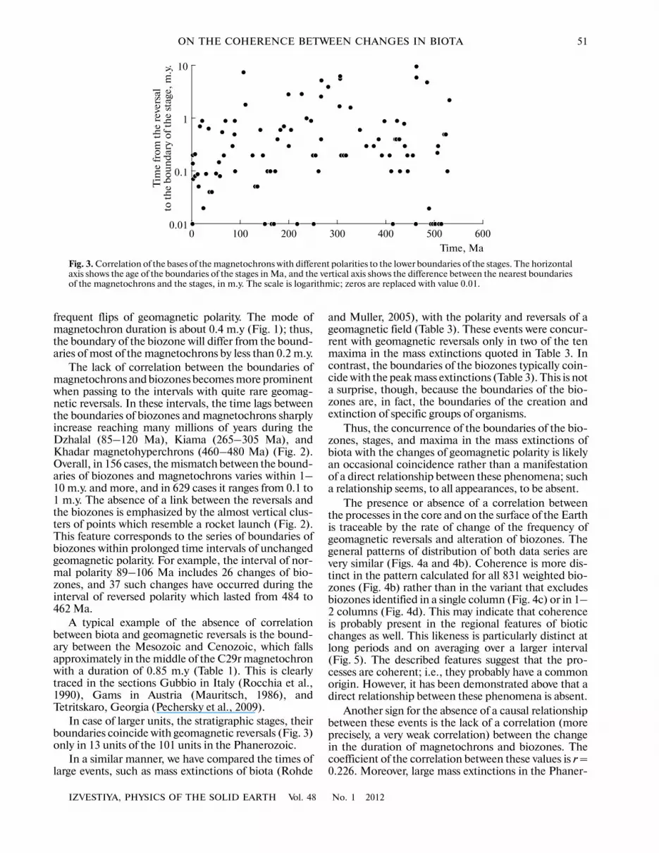
In case of larger units, the stratigraphic stages, theirboundaries coincide with geomagnetic reversals (Fig. 3)only in 13 units of the 101 units in the Phanerozoic.

In a similar manner, we have compared the times oflarge events, such as mass extinctions of biota (Rohde

and Muller, 2005), with the polarity and reversals of ageomagnetic field (Table 3). These events were concur�rent with geomagnetic reversals only in two of the tenmaxima in the mass extinctions quoted in Table 3. Incontrast, the boundaries of the biozones typically coin�cide with the peak mass extinctions (Table 3). This is nota surprise, though, because the boundaries of the bio�zones are, in fact, the boundaries of the creation andextinction of specific groups of organisms.

Thus, the concurrence of the boundaries of the bio�zones, stages, and maxima in the mass extinctions ofbiota with the changes of geomagnetic polarity is likelyan occasional coincidence rather than a manifestationof a direct relationship between these phenomena; sucha relationship seems, to all appearances, to be absent.

The presence or absence of a correlation betweenthe processes in the core and on the surface of the Earthis traceable by the rate of change of the frequency ofgeomagnetic reversals and alteration of biozones. Thegeneral patterns of distribution of both data series arevery similar (Figs. 4a and 4b). Coherence is more dis�tinct in the pattern calculated for all 831 weighted bio�zones (Fig. 4b) rather than in the variant that excludesbiozones identified in a single column (Fig. 4c) or in 1–2 columns (Fig. 4d). This may indicate that coherenceis probably present in the regional features of bioticchanges as well. This likeness is particularly distinct atlong periods and on averaging over a larger interval(Fig. 5). The described features suggest that the pro�cesses are coherent; i.e., they probably have a commonorigin. However, it has been demonstrated above that adirect relationship between these phenomena is absent.

Another sign for the absence of a causal relationshipbetween these events is the lack of a correlation (moreprecisely, a very weak correlation) between the changein the duration of magnetochrons and biozones. Thecoefficient of the correlation between these values is r =0.226. Moreover, large mass extinctions in the Phaner�

00.01

100 200 300 400 500 600

0.1

1

10

Time, Ma

Tim

e fr

om t

he

reve

rsal

to t

he

boun

dary

of t

he

stag

e, m

.y.

Fig. 3. Correlation of the bases of the magnetochrons with different polarities to the lower boundaries of the stages. The horizontalaxis shows the age of the boundaries of the stages in Ma, and the vertical axis shows the difference between the nearest boundariesof the magnetochrons and the stages, in m.y. The scale is logarithmic; zeros are replaced with value 0.01.

52

IZVESTIYA, PHYSICS OF THE SOLID EARTH Vol. 48 No. 1 2012

PECHERSKY et al.

ozoic occurred during a very diverse state of geomag�netic field and do not tell on the frequency of biozones(Figs. 4a, 4b, and 6a). This fact perhaps reflects differ�ent phenomena: on one hand, natural evolution of life,which shows in the rate of change of biozones, and, onthe other hand, catastrophic extinctions superimposedon the first process. A similar situation is also observedwith the maxima of diversity which occurred duringvarious geomagnetic conditions (Figs. 4a and 6b). Thefrequency of the alteration of biozones (Figs. 4b and6b) exhibits a more moderate pattern: most of thediversity maxima correspond to the intervals whenthere were 1–2 biozones during 1 m.y.

The favorable environmental conditions whichfacilitated the rise of the diversity in the life forms areprobably manifested in the lifetime of each of thegroups of the organisms as well.

The rhythmicity of the pattern is worth noting: peri�ods of enhanced activity in the core and on the surfaceof the Earth regularly and almost synchronically alter�nate with quiet intervals with rare geomagnetic reversalsand much longer durations of biozones. A particularemphasis should be placed on the striking similarity andsynchronism of the long intervals with rare reversals andrare alterations of biozones. Namely, these are the inter�vals of 80–120, 200–240, 270–310, 340–380, and470–490 Ma. The likeness in the general patterns ofthese events, primarily, points to the coherence betweenthe long�lasting rather than short�scale processes. Theincrease in the coefficient of correlation from r = 0.226(averaging interval 3 m.y.) to 0.375 (averaging interval9 m.y.) also reflects this feature.

The situation with short�scale variations in the num�ber of the geomagnetic reversals and the frequency ofthe biozone alterations is much worse. As seen fromFig. 4, in some cases, the peaks in both these time seriescoincide, while in other cases the maxima in the fre�

quency of reversals either lag behind or precede the fre�quency of the biozonal changes. The probable source ofthese discrepancies is the uncertainty in correlating thebiozones to the magnetostratigraphic scale. However,the coefficient of correlation consistently increases asthe time lag between the time series of geomagneticreversals and the time series of biotic changes increasesby 3–8 m.y.; after this, the coefficient of correlationdecreases as the time lag further increases (Table 4). Inother words, a tendency of the change rate of the fre�quency of geomagnetic reversals insignificantly laggingthe frequency of biozonal changes by 6 m.y. starts toappear.

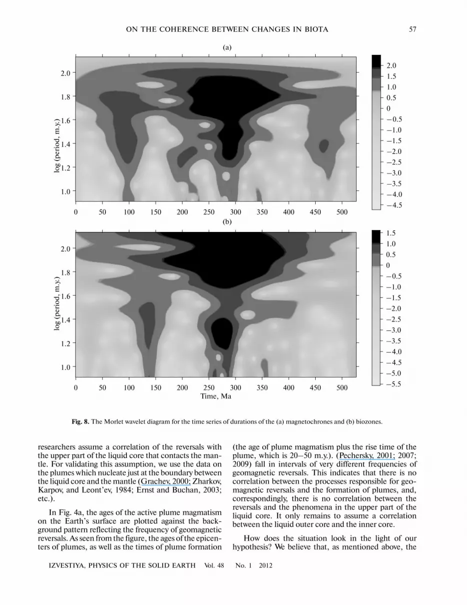
The coherence in the rate of change of the geomag�netic reversals and biozonal alterations is reflected inthe power spectra of these data (Fig. 7), which containa number of frequency components, some of whichcoincide or are very similar, namely, the periods of 16,20, ~30, ~50, 60–70, and 90–100 m.y. (Fig. 7). Thedark cloud on the wavelet diagram (Fig. 8) reflects themain oscillations which are common in the magneto�chrons and biozones. The following rhythms are recog�nized in the duration of the magnetochrons: a period of90 m.y. in the interval from 500 to 50 Ma; a period of65 m.y. in the interval 530–0 Ma; a period of 50 m.y. inthe interval 400(?)–50(?) Ma; a period of 30 m.y. in theintervals 140–60 Ma and 370–230 Ma; and a period of20 m.y. in the intervals 120–70 Ma, 230–150 Ma, and320–260 Ma. The biozonal durations were found tocontain the following rhythms: a period of 80–90 m.y.in the interval 480–0 Ma; a period of 60 m.y. in theinterval 430–220 (?) Ma; a period of 50 m.y. in theinterval 300 (?)–50 Ma; a period of 30 m.y. in the inter�vals 160–90 Ma and 400–250 (?) Ma; and a period of20 m.y. in the intervals 160–110 Ma and 310–240 Ma.The shorter�period oscillations, which are clearly dis�tinguished in the power spectra, are vague in the wavelet

Table 3. Correlation of the ages of maximal mass extinctions to the ages of the nearest geomagnetic reversals and bound�aries of the biozones

Maximum, Ma Polarity Reversal, base Reversal, top Biozone, base Biozone, top

33.9 R 34.26 32.01 33.9 33.9

65.5 (big 5) R 65.7 64.85 65.5 65.5

145.5 R 145.8 145.3 145.5 145.5

199.6 (big 5) N 202.3 199.3 199.6 199.6

251 (big 5) NR 251 251 251 251

323.5 R 323.9 323.3 324.3 323.3

374.5 (big 5) R 374.8 371.5 374.5 374.5

416 NR 416 416 416 416

443.7 (big 5) R 445.5 443.5 443.7 443.7

518.7 N 518.9 518.5 518.7 518.7

Note: maximum is the age of peak mass extinction, Ma (Rohde and Muller, 2005); polarity is the polarity of the geomagnetic field duringthe peak mass extinction; N is normal polarity; R is reversed polarity; NR is the geomagnetic reversal. Reversal stands for the ageof the nearest geomagnetic reversal; biozone is the age of the boundary of biozone, which is closest to the maximum extinction;base means earlier than the peak extinction; top means later than the peak extinction.

IZVESTIYA, PHYSICS OF THE SOLID EARTH Vol. 48 No. 1 2012

ON THE COHERENCE BETWEEN CHANGES IN BIOTA 53

0 50 100 150 200 250 300 350 400 450 500 550

2

4

6

8

10

14N

0 50 100 150 200 250 300 350 400 450 500 550

1

2

3

4

5

6

Time, Ma

N7

(а)

(b)

12

0 50 100 150 200 250 300 350 400 450 500 550

1

2

3

5

Time, Ma

N( weight)

4

0 50 100 150 200 250 300 350 400 450 500 550

2

4

6

8

10

14

N

12

14

(c)

(d)

Fig. 4. Correlation of (a) the frequency of reversals to (b, c, d) the boundaries of biozones, averaging over 3 m.y. with a shift by1 m.y. The graphs are based on the data from Tables 1 and 2, respectively. The dataset for graph 4b comprises the biozones withcorresponding weights (see the text and notes to Table 2); graph 4c reflects the results with excluded biozones determined in asingle stratigraphic column only; graph 4d corresponds to the data with excluded biozones identified in 1–2 columns. The verticalarrows below the horizontal axis in Fig. 4a mark the episodes of magmatism on the Earth’s surface associated with the lower�man�tle plume activity (Ernst and Buchan, 2003; Grachev, 2003). The arrows in the upper part of Fig. 4b indicate the maxima in themass extinctions of biota (Raup and Sepkoski, 1982; Rohde and Muller, 2005).

54

IZVESTIYA, PHYSICS OF THE SOLID EARTH Vol. 48 No. 1 2012

PECHERSKY et al.

diagram where they only form some diffuse splashes. Allthis indicates that the series of oscillations with periodsof about 50 m.y. and longer cover a large part of thePhanerozoic, whereas oscillations with periods shorterthan 30 m.y. occur during relatively short intervals(Fig. 8). The likeness of the patterns for magnetochronsand biozones is remarkable.

We have figured out the degree of frequency�depen�dent synchronism of oscillations in both time series byestimating the symmetric magnitude�squared spectralcoherence. It is seen in Fig. 9 that several periods (10,14, 16, and 55–60 m.y.) are highly synchronous andtheir squared coherence is, respectively, 0.56 (r = 0.74),0.59 (r = 0.77), 0.66 (r = 0.81), and 0.76 (r = 0.87),

0 50 100 150 200 250 300 350 400 450 500 550

2

4

6

8

10

12

Time, Ma

N

0 50 100 150 200 250 300 350 400 450 500 550

2

4

6

8

10

12

Time, Ma

N(weight)

14

16

18

20

(а)

(b)

Fig. 5. Correlation of the frequency of (a) magnetochrons to the (b) biozones with averaging in a 9�m.y. window shifted by 1 m.y.Graph 5b for biozones is based on the weighted data (see the text and the notes to Table 2).

Table 4. The dependence of the coefficient of linear correlation between the geomagnetic reversal and biozone scales onthe time shift of the former relative to the latter

(A) averaging interval 3 m.y.

shift 0 3 4 5 6 7 8 9 15

r 0.226 0.234 0.226 0.226 0.228 0.23 0.211 0.164 0.04

shift 0 –3 –4 –5 –6 –7 –8 –9 –10

r 0.226 0.227 0.230 0.254 0.254 0.235 0.239 0.246 0.244

(B) averaging interval 9 m.y.

shift 0 3 4 5 6 7 8 9 15

r 0.375 0.357 0.347 0.335 0.319 0.3 0.278 0.252 0.071

shift 0 –3 –4 –5 –6 –7 –8 –9 –10

r 0.375 0.383 0.385 0.388 0.389 0.388 0.38 0.371 0.36

IZVESTIYA, PHYSICS OF THE SOLID EARTH Vol. 48 No. 1 2012

ON THE COHERENCE BETWEEN CHANGES IN BIOTA 55

which is far above the values typical for other periods.Here, the phase shift of the coherent oscillations rangesfrom zero to 10–15 m.y. of magnetochrons either lag�ging or preceding biozones. We recall that the phaseshift by 3–8 m.y. of the time series of magnetochronswith respect to the time series of biozones is identifiedagainst an increase in the coefficient of correlation(Table 4). Obviously, in the latter case, we have the inte�gral result contributed by all oscillations, and this resultprovides a more adequate view of the real situation.

Even with noticeable averaging and shifting by 6 m.y.,the coefficient of correlation barely attains 0.39; i.e., theprobability of such shift is as small as 0.15.

Thus, on one hand, there is no correlation betweenthe reversals (i.e., major changes in the magnitude anddirection of the geomagnetic field) and the biozones(i.e., changes in the organic world). On the other hand,the rate of change of both these processes shows a dis�tinct coherence close to synchronism. Therefore, thesynchronism of the processes does not necessarily tes�

0 50 100 150 200 250 300 350 400 450 500 542

10

20

30

40

50

60

0

0

50 100 150 200 250 300 350 400 450 500 542

1

2

3

4

5

N Pg K J Tr P C D S O Cm

Intensity of extinction, %

Time, Ma

Time, Ma

Thousands of genera

(a)

(b)

Fig. 6. The intensity of (a) mass extinctions and (b) diversity of marine organisms in the Phanerozoic (Raup and Sepkoski, 1982;Rohde and Muller, 2005).

56

IZVESTIYA, PHYSICS OF THE SOLID EARTH Vol. 48 No. 1 2012

PECHERSKY et al.

tify to their causal relationship. At the same time, thecommon source of the revealed coherent changes isquite probable. A probable common source of thecoherence between the mutually independent processesoriginating in the core (geomagnetic reversals) andoccurring on the Earth’s surface (events in the bio�sphere) is the rotation of the Earth. The global changesin the organic world may well be due to long�lastingchanges in the rotation velocity and axial tilt of theEarth. For example, it has been noticed that the onsetand termination of geomagnetic excursions fall in theperiods of climatic changes (Wollin et al., 1971; Bowen,1978; Pospelova, 2000); the periods of variations in themagnitude and direction of the geomagnetic field coin�cide with the periods of variations in the magnetic char�acteristics that reflect climatic changes (Pospelova,2000).

The Phanerozoic is clearly dominated by thereversed geomagnetic polarity (Table 1). Apparently,this reflects the fact that the Earth was always rotating inthe same direction as it does today, i.e., counterclock�wise. Against this background, according to the fractalanalysis of the magnetochronostratigraphic scale(Pechersky, Reshetnyak, and Sokoloff, 1997; Pecher�sky, 2009), two regimes of generation of the geomag�netic field existed during this time. The first is theregime of frequent reversals, which is chaotic (the frac�tal dimension d < 0.6), and the second is the regime ofstable field state with rare, up to no reversals, which pos�sesses a clear self�similarity (d close to unity). The infer�ences of the fractal analysis are supported by theresults of wavelet study: the periods shorter than50 m.y., which are revealed in the time series of thefrequency of geomagnetic reversals and the fre�

quency of the alteration of biozones during the Phan�erozoic, are relatively short events, whose time distri�bution appear to be rather chaotic.

We need a hypothesis that would account for the tworegimes of geomagnetic field generation, on one hand,and for the coherence of processes occurring in the coreand on the surface of the Earth, on the other hand. Wemay seek to associate both these points with the rotationof the solid inner core of the Earth relative to the man�tle. For this, first, we consider nonuniformity in theEarth’s rotation. There is evidence from astronomy thatover the past 2700 years, the retardation of the Earth’srotation averaged 0.002 s per 100 years, and over thepast 250 years, it was 0.0014 s/100 years. During the lat�est three decades, the rotation of the Earth is accelerat�ing, and jumps in the rotation velocity of up to 0.004 soccur (Sidorenkov, 2004). With the average retardationassumed to be 0.002 s per 100 years, the retardation ofthe rotation over the entire Phanerozoic will be about3 hours (0.002 × 540 Ma). This value agrees with theestimate obtained, e.g., by Munk and MacDonald(1960).

Second, it is reasonable to suppose the rotation ofthe inner core of the Earth to either lag or precede themantle, depending on the acceleration or retardation ofthe latter, due to a liquid “gasket” between the core andthe mantle, as it is theoretically demonstrated in (Gro�ten and Molodensky, 1999). It follows from the complexof observations that the inner core is moveable and itsaxial rotation differs from the rotation of the wholeEarth (Avsyuk, Adushkin, and Ovchinnikov, 2001).Third, it is necessary to explore the possible correlationbetween the geomagnetic reversals and interactions ofthe liquid and solid inner core of the Earth. Most

1000

40

80

120

10 1000

10

20

30

10Period, m.y.

(а) (b)

Period, m.y.

Fig. 7. The power spectral estimates for the time series of (a) magnetochrons and (b) biozones.

IZVESTIYA, PHYSICS OF THE SOLID EARTH Vol. 48 No. 1 2012

ON THE COHERENCE BETWEEN CHANGES IN BIOTA 57

researchers assume a correlation of the reversals withthe upper part of the liquid core that contacts the man�tle. For validating this assumption, we use the data onthe plumes which nucleate just at the boundary betweenthe liquid core and the mantle (Grachev, 2000; Zharkov,Karpov, and Leont’ev, 1984; Ernst and Buchan, 2003;etc.).

In Fig. 4a, the ages of the active plume magmatismon the Earth’s surface are plotted against the back�ground pattern reflecting the frequency of geomagneticreversals. As seen from the figure, the ages of the epicen�ters of plumes, as well as the times of plume formation

(the age of plume magmatism plus the rise time of theplume, which is 20–50 m.y.). (Pechersky, 2001; 2007;2009) fall in intervals of very different frequencies ofgeomagnetic reversals. This indicates that there is nocorrelation between the processes responsible for geo�magnetic reversals and the formation of plumes, and,correspondingly, there is no correlation between thereversals and the phenomena in the upper part of theliquid core. It only remains to assume a correlationbetween the liquid outer core and the inner core.

How does the situation look in the light of ourhypothesis? We believe that, as mentioned above, the

Fig. 8. The Morlet wavelet diagram for the time series of durations of the (a) magnetochrones and (b) biozones.

2.0

1.5

1.0

0.5

0

–0.5

–1.0

–1.5

–2.0

–2.5

–3.0

–3.5

–4.0

–4.5

1.5

1.0

0.5

0

–0.5

–1.0

–1.5

–2.0

–2.5

–3.0

–3.5

–4.0

–4.5

–5.0

–5.5

0

2.0

1.8

1.6

1.4

1.2

1.0

50 100 150 200 250 300 350 400 450 500

0

2.0

1.8

1.6

1.4

1.2

1.0

50 100 150 200 250 300 350 400 450 500

(а)

(b)

Time, Ma

log

(per

iod,

m.y

.)lo

g (p

erio

d, m

.y.)

58

IZVESTIYA, PHYSICS OF THE SOLID EARTH Vol. 48 No. 1 2012

PECHERSKY et al.

dominant reversed geomagnetic polarity is due to thecounterclockwise rotation of the Earth. This polaritywill persist if the inner core, the outer core, and themantle rotate synchronously, or if the inner core pre�cedes the remaining parts of the Earth. During the peri�ods of acceleration of the Earth’s rotation, when theinner core rotates slower than the mantle, a relativecounterrotation appears at the boundary between thesolid and liquid core, and, correspondingly, the fieldassociated with this counterrotation must have theopposite sign; i.e., the same sign as the present�dayfield. Therefore, the long intervals of stable polarity ofthe geomagnetic field reflect the steady regime of theEarth’s rotation. More frequently, it is a consistentretardation, which agrees with the data of astronomical,geophysical, and geological observations; far rarer, it isa stable acceleration (the Dzhalal hyperchron of normalpolarity).

Both these phenomena characterize the long�periodrhythm in the generation of the geomagnetic field witha period of about 180–190 m.y. (fractal dimension ofabout unity), likely of a galactic scale. At the same time,the intervals of frequent flips in the geomagnetic polar�

ity relate to an unstable, close to chaotic, regime in theEarth’s rotation (fractal dimension below 0.6), whenretardation of the rotation frequently changes by accel�eration. This regime has long lasted during the Phaner�ozoic. Against the background of predominantlyreversed geomagnetic polarity, i.e., counterclockwiserotation of the Earth, there were intervals with unstablegeomagnetic polarity: the early Paleozoic (530–483),middle Paleozoic (468–315 Ma), Mesozoic (258–123 Ma), and Cenozoic (83–0 Ma) (Table 1 (Molos�tovskii, Pechersky, and Frolov, 2007)). The changes inthe Earth’s rotation velocity should have manifestedthemselves in the synchronous behavior of the processesoccurring on the surface and in the core of the Earth,which is what we see in our example of coherence in thefrequencies of geomagnetic reversals and the changes inthe boundaries of the biozones.

CONCLUSIONS

(A) From the data on the geomagnetic reversals, thebiozones, the geological stages, and the maxima in themass extinctions of the biota in the Phanerozoic, which

1000

0.2

0.4

0.8

10 Period, Ma

0.6

M2

Fig. 9. The estimate of magnitude�squared spectral coherence (vertical axis, M2) between the time series of magnetochrons andbiozones.

IZVESTIYA, PHYSICS OF THE SOLID EARTH Vol. 48 No. 1 2012

ON THE COHERENCE BETWEEN CHANGES IN BIOTA 59

are cited in the present paper, it follows that a direct cor�relation between these events is absent. The boundariesof the geological stages, periods, ages, and biozones,and the peaks in the mass extinctions are typically notmarked by changes in geomagnetic polarity. At the sametime, a coherent, close to synchronous pattern of thefrequency of alteration of biozones and geomagneticpolarity is observed. Synchronism of these processes isindicated by a number of common spectral components(with periods from 10 to 80–90 m.y.) revealed in thesetime series. The synchronism of the periods of 10, 14,16, and 60 m.y. is quantitatively demonstrated in thechanges of geomagnetic polarity and in the boundariesof biozones.

The times of plume formation correspond to theintervals with a very different frequency of geomagneticreversals. This fact suggests that the sources of plumesand geomagnetic reversals are different. So long as thenucleation and formation of plumes is confined to theboundary between the core and the mantle of the Earth,it is reasonable to assume that the change in the sign ofthe field is the result of the interaction between the liq�uid and solid core. We suggest that the regular coherentrhythmicity in the changes of geomagnetic polarity andboundaries of biozones is associated with the variationsin the rotation velocity of the inner core of the Earthand the tilt of the axis of its rotation relative to the man�tle. Correspondingly, the long intervals of stable geo�magnetic polarity reflect the steady regime of theEarth’s rotation, whereas the intervals with frequentreversals relate to unstable rotation when retardationfrequently changes to acceleration. Such a regimelasted for a long time during the Phanerozoic when itwas superimposed on the background dominance ofreversed polarity that corresponds to the counterclock�wise rotation of the Earth.

The changes in the Earth’s rotation and in the tilt ofits rotational axis, which are responsible for the syn�chronous pattern of the change rates of the duration ofmagnetochrons and biozones are probably associatedwith the tidal evolution of the Moon�Earth system, aswell as the evolution of the Earth in the solar system andin the general development of the Galaxy.

(B) To what extent is the development, evolution ofliving nature, due to the geomagnetic field?

The lack of a direct correlation between the changesin the biosphere with the large variations in the magni�tude and direction of the geomagnetic field during thePhanerozoic, apparently, indicates that the geomag�netic field had no effect on the evolution of life on theEarth. This also follows from the fact that life on Earthhas consistently progressed from the primitive unicellu�lar forms to mammals and humans, and its diversity hasgrown against an approximately similar backgroundgeomagnetic field during 2.5 Ga (Shcherbakov andSycheva, 2006; Pechersky, Zakharov, and Lyubushin,2004) and independently of repeated reversals.

Moreover, the evolution of life was deterministic,despite the large catastrophic events in the history of the

Earth. The biological clock that developed in the courseof evolution has worked and keeps working perfectly:individual organisms and species are born, live, and die.There are dayflies, there are plants that live for a year,there are plants and animals that live to many hundredsof years, and this does not depend on catastrophicevents—catastrophes do not break the mechanism ofevolution of life once set in motion.

Thus, the evolution of life on Earth neitherdepends on large changes in the geomagnetic fieldnor on extreme catastrophic events that lead to themass extinctions of biota. This is the main conclusion ofour work.

ACKNOWLEDGMENTS

We are grateful to A.S. Alekseev, A.F. Grachev, andA.Yu. Guzhikov for carefully reading the paper andtheir valuable comments and recommendations.

REFERENCES

Avsyuk, Yu.N., Adushkin, V.V., and Ovchinnikov, V.M.,Multidisciplinary Study of the Mobility of the Earth’s InnerCore, Izv. Phys. Earth, 2001, vol. 37, no. 8, pp. 673–683.Bowen, D.Q., QuaternaryGeology: A Stratigraphic Frame�work for Multidisciplinary Work,Oxford, UK: Pergamon,1978.Brillinger, D.R., Time series. Data Analysis and Theory,New York: Holt, Rinehart and Winston, 1975.Ernst, R.E. and Buchan, K.L., Recognizing Mantle Plumesin the Geological Record, Annu. Rev. Earth Planet. Sci.,2003, vol. 31, pp. 469–523.Grachev, A.F., Mantle Plumes and Problems of Geody�namics, Izv. Phys. Earth, 2000, vol. 36, no. 4, pp. 263–294.Grachev, A.F., Identification of Mantle Plumes Based onthe Study of Isotopic and Geochemical Characteristics ofVolcanic Rocks, Petrology, 2003, vol. 11, no. 6, pp. 618–654.Gradstein, F.M., Ogg, J., and van Kranendonk, M., On theGeological Time Scale 2008, Newslett. Stratigraphy, 2008,vol. 43, no. 1, pp. 5–13.Groten, E. and Molodensky, S.M., On the Mechanism ofthe Secular Tidal Acceleration of the Solid Inner Core andthe Viscosity of the Liquid Core, Stud. Geophys. Geodet.,1999, vol. 43, pp. 20–34.Guzhikov, A.Yu., Baraboshkin, E.Yu., and Birbina, A.V.,New Paleomagnetic Data for the Hauterivian�AptianDeposits of the Middle Volga Region: a Possibility of GlobalCorrelation and Dating of Time�Shifting of StratigraphicBoundaries, Rus. J. Earth Sci., 2003, vol. 5, no. 6, pp. 401–430.Guzhikov, A.Yu., Paleomagnetic Scale and Magnetism ofthe Jurassic�Carboniferous Rocks in the Russian Plate andAdjacent Territories, Extended Abstract of Doct. Sci. Disser�tation (Geol. Mineral.), Trofimuk Institute Of PetroleumGeology and Geophysics, Siberian Branch of the RussianAcademy of Science, Novosibirsk, 2004.Khramov, A.N. and Shkatova, V.K., General Magneto�stratigraphic Scale of Polarity for the Phanerozoic, inDopolneniya k stratigraf. kodeksu Rossii (Suppl. to Strati�

60

IZVESTIYA, PHYSICS OF THE SOLID EARTH Vol. 48 No. 1 2012

PECHERSKY et al.

graphic Code of Russia), St. Petersburg: VSEGEI, 2000,pp. 34–45.Lyubushin, A.A., Analiz dannykh sistem geofizicheskogo iekologicheskogo monitoringa (Analysis of the Data from theSystems of Geophysical and Ecological Monitoring), Mos�cow: Nauka, 2007.Mauritsch, H.J., Der Stand Der Palaomagnetischen Fors�chung in Den Ostaplen, Leobner Hefte fur Angewandte Geo�physik, 1986, vol. 1, pp. 141–160.Molostovskii, E.A., Pechersky, D.M., and Frolov, I.Yu.,Magnetostratigraphic Timescale of the Phanerozoic and ItsDescription Using a Cumulative Distribution Function,Izv. Phys. Earth, 2007, vol. 43, no. 10, pp. 811–818.Munk, W. and MacDonald, G.J.F., The Rotation of theEarth: A Geophysical Discussion, Cambridge: CambridgeUniv. Press, 1960.Pavlov, V. and Gallet, Y., A Third Superchron during theEarly Paleozoic, Episodes, 2005, vol. 28, no. 2, pp. 1–7.Pechersky, D.M., Reshetnyak, M.Yu., and Sokoloff, D.D.,A Fractal Analysis of the Time Scale of Geomagnetic Polar�ities, Geomagn. Aeron., 1997, vol. 37, no. 4, pp. 490–497.Pechersky, D.M., Neogeaen Paleomagnetism: Constraintson the Processes at the Core and Surface of the Earth, Rus.J. Earth Sci., 1998, vol. 1, no. 2, pp. 103–135.Pechersky, D.M., Changes in the Organic World and Geo�magnetic Field during the Vendian–Phanerozoic, Stratigr.Geol. Correlation, 2000, vol. 8, no. 2, pp. 206–210.Pechersky, D.M., The Total Amplitude of Secular Varia�tions, Global Magnetic Anomalies and Plumes, Izv. Phys.Earth, 2001, vol. 37, no. 5, pp. 429–435.Pechersky, D.M., Zakharov, V.S., and Lyubushin, A.A.,Continuous Record of Geomagnetic Field Variations dur�ing Cooling of the Monchegorsk, Kivakka and BushveldEarly Proterozoic Layered Intrusions, Rus. J. Earth Sci.,2004, vol. 6, no. 6, pp. 391–456.Pechersky, D.M. and Garbuzenko, A.V., The Mesozoic�Cenozoic Boundary: Paleomagnetic Characteristic, Rus. J.Earth Sci., 2005, vol. 7, no. 2, pp. 1–15.Pechersky, D.M., The Geomagnetic Field at the Paleo�zoic/Mesozoic and Mesozoic/Cenozoic Boundaries andLower Mantle Plumes, Izv. Phys. Earth, 2007, vol. 43,no. 10, pp. 844–854.

Pechersky, D.M., The Geomagnetic Field at the Protero�zoic–Paleozoic Boundary and Lower�Mantle Plumes, Izv.Phys. Earth, 2009, vol. 45, no. 1, pp. 14–20.Pechersky, D.M., Asanidze, B.Z., Nourgaliev, D.K., andSharonova, Z.V., Petromagnetic and Paleomagnetic Char�acterization of Mesozoic/Cenozoic Deposits: TheTetritskaro Section (Georgia), Izv. Phys. Earth, 2009,vol. 45, no. 2, pp. 134–149.Pechersky, D.M., Lyubushin, A.A., and Sharonova, Z.V.,On the Synchronism in the Events within the Core and onthe Surface of the Earth: the Changes in the Organic Worldand in the Polarity of the Geomagnetic Field in the Phaner�ozoic, Izv. Phys. Earth, 2010, vol. 46, no. 7, pp. 613–623.Pospelova, G.A., Geomagnetic Excursions of the BrunhesChron and Global Climate Oscillations, Izv. Phys. Earth,2000, vol. 36, no. 8, pp. 619–629.Raup, D. and Sepkoski, J., Mass Extinctions in the MarineFossil Record, Science, 1982, vol. 215, pp. 1501–1503.Rohde, R.A. and Muller, R.A., Cycles in the Fossil Diver�sity, Nature, 2005, vol. 434, pp. 209–210.Rozanov, A.Yu., Semikhatov, M.A., Sokolov, B.S., andKhomentovskii, V.V., The Decision on the Precambrian–Cambrian Boundary Stratotype: A Breakthrough or Mis�leading Action?, Stratigr. Geol. Correlation, 1997, vol. 5,no. 1, pp. 19–28.Roñchia, R., Boclet, D., Bonte, Ph., Jehanno, C., Chen, Y.,Courtillot, V., Mary, C., and Wezel, F., The Cretaceous�Tertiary boundary at Gubbio Revisited: Vertical Extent ofthe Ir Anomaly, Earth Planet. Sci. Lett., 1990, vol. 99,pp. 206–219.Shcherbakov, V.P. and Sycheva, N.K., On the Variation inthe Geomagnetic Dipole over the Geological History of theEarth, Izv. Phys. Earth, 2006, vol. 42, no. 3, pp. 201–206.Sidorenkov, N.S., Instability of the Earth’s Rotation, Her�ald Russ. Acad. Sci. (Transl. of Vestn. Ross. Akad. Nauk),2004, vol. 74, no. 4, pp. 402–409.Wollin, E., Ericson, D.B., Ryan, W.B.F., and Foster, G.H.,Magnetism of the Earth and Climatic Changes, EarthPlanet. Sci. Lett., 1971, vol. 12, no. 2, pp. 175–183.Zharkov, V.N., Karpov, P.B., and Leont’ev, V.V., On a Ther�mal Regime of the Core–Mantle Boundary Layer, Dokl.Akad. Nauk SSSR, 1984, vol. 275, pp. 335–338.