arX

iv:0

908.

2460

v1 [

astr

o-ph

.SR

] 1

7 A

ug 2

009

Parameters of the Magnetic Flux inside Coronal Holes

Valentyna Abramenko and Vasyl YurchyshynBig Bear Solar Observatory, Big Bear City, CA 92314, USA

Hiroko WatanabeKwasan and Hida Observatories, Kyoto University, Kitakazan, Ohminecyou,

Yamashina, Kyoto 607-8471, Japan

Abstract. Parameters of magnetic flux distribution inside low-latitude coronalholes (CHs) were analyzed. A statistical study of 44 CHs based on Solar andHeliospheric Observatory (SOHO)/MDI full disk magnetograms and SOHO/EIT284A images showed that the density of the net magnetic flux, Bnet, does notcorrelate with the associated solar wind speeds, Vx. Both the area and net fluxof CHs correlate with the solar wind speed and the corresponding spatial Pearsoncorrelation coefficients are 0.75 and 0.71, respectively. A possible explanation forthe low correlation between Bnet and Vx is proposed. The observed non-correlationmight be rooted in the structural complexity of the magnetic field. As a measureof complexity of the magnetic field, the filling factor, f(r), was calculated as afunction of spatial scales. In CHs, f(r) was found to be nearly constant at scalesabove 2 Mm, which indicates a monofractal structural organization and smoothtemporal evolution. The magnitude of the filling factor is 0.04 from the HinodeSOT/SP data and 0.07 from the MDI/HR data. The Hinode data show that at scalessmaller than 2 Mm, the filling factor decreases rapidly, which means a mutlifractalstructure and highly intermittent, burst-like energy release regime. The absenceof necessary complexity in CH magnetic fields at scales above 2 Mm seems to bethe most plausible reason why the net magnetic flux density does not seem to berelated to the solar wind speed: the energy release dynamics, needed for solar windacceleration, appears to occur at small scales below 1 Mm.

Keywords: Sun: magnetic fields, coronal holes, solar wind

1. Introduction

Since the Skylab mission in early 1970s, it is believed that the coronalholes seen on the surface of the Sun are related to the high-speedstreams of the solar wind and they might be a cause of geomagneticdisturbances (see, e.g., Sheeley et al. (1976) and references therein). Apossibility of ground-based observations of coronal holes in the spectralline He 1083.0 nm (Harvey et al., 1975) stimulated the interest tothe problem. Numerous sophisticated models were proposed to explainthe CHs formation and evolution (e.g., Wang and Sheeley, 1991; Fisk,1996, 2001, 2005; Fisk et al., 1999; Wang et al., 2000; Schrijver, 2001;Schrijver and Title, 2001; Schrijver et al., 2002; Schrijver and DeRosa,2003).

c© 2009 Kluwer Academic Publishers. Printed in the Netherlands.

ms14.tex; 18/08/2009; 18:01; p.1

2

During the last decade, a connection between the coronal holes andvarious heliospheric phenomena, such as, high speed streams, corotat-ing interaction regions, long-living geomagnetic storms without CMEs(see, e.g., Vrsnak et al., 2007 for references), became well establishedand stimulated elaboration of approaches to forecast the geomagneticresponse to the transit of a coronal hole over the solar disk. An areaoccupied by coronal holes turned to be a very fruitful parameter. Rob-bins et al. (2006) suggested an empirical model to predict the solarwind speed at 1 AU from measurements of the fractional area occupiedby a CH inside a 14◦ - sectoral region centered at the central meridian.A similar technique was independently applied later by Vrsnak et al.

(2007) and further extended to forecast, along with the solar windspeed, other parameters of the solar wind, such as proton density,temperature and magnetic field strength at 1 AU.

Several groups analyzed properties of the magnetic fields insidecoronal holes (e.g., Harvey and Sheeley, 1979; Harvey et al., 1982;Obridko and Shelting, 1989; Bumba et al., 1995; Obridko et al., 2000;Wiegelmann and Solanki, 2004; Wiegelmann et al., 2005; Abramenkoet al., 2006; Hagenaar et al., 2008). The most comprehensive studymade so far on the net magnetic fluxes and averaged flux densities incoronal holes was presented by Harvey and colleagues (Harvey et al.,1982), which was based on the Kitt Peak full disk magnetograms (1arcsec pixel size) and hand-drawn maps of coronal holes derived fromthe He 1083.0 nm data. These authors analyzed the ascending phase ofthe 21st cycle and reported an increase in the averaged net flux densityas the solar activity intensified. This was explained by an extra fluxdeposited into low-latitude coronal holes by decaying active regions.Since then, the density of the net flux inside CHs was adopted as arepresentative characteristic of the magnetic filed inside coronal holes.

As long as it is the magnetic field that is ultimately responsible forenergetics in a coronal hole, it would be interesting to explore howthe density of the net magnetic flux is related to the speed of thefast solar wind. We performed such a statistical study on the basisof the MDI full disk magnetograms (Section 2) and found a rathersurprising result: the density of the net flux is not correlated withthe solar wind speed measured at 1 AU. What could be a reason forthat? We suggested that the reason might be that the density of themagnetic flux, derived from low-resolution data and averaged over theCH’s area, is not a suitable parameter to qualify energetics in CHs. Theultimate reason for the observed non-correlation might stem from thestructural organization of the magnetic flux and its multifractal natureat small scales. This encouraged us to study multifractal properties ofthe magnetic flux inside a coronal hole taking advantage of the high

ms14.tex; 18/08/2009; 18:01; p.2

3

resolution Hinode observations of the magnetic field (Section 3). Ourfinal section represents summary and discussion of the results.

2. Averaged Net Flux Density Versus the Solar Wind

Speed

2.1. Event Selection

Here we focus on the distribution of the magnetic flux density of 44CHs observed between March 2001 and July 2006 at low solar latitudesnear the center of the solar disk (Table I). To avoid influence of theprojection effect, we required that the angular distance, θ, from the diskcenter to the center of gravity of a CH should not exceed 20 degrees.The values of θ (positive when the gravity center was located in thenorthern hemisphere) are shown in the 8-th column of Table I. In theprocess of event selection we discarded all CHs that had more than 5%of their area outside a circle of 30 degree radius centered at the solardisk center.

We also made sure that the solar wind speed profiles were notcontaminated by a possible influence of ICMEs. Following Arge et al.

(2004), we selected only the events when, at the arrival time of thestreams, the value of the plasma beta(http : //omniweb.gsfc.nasa.gov/form/dx1.html) was well above 0.1.

For the selected 44 CHs (Table I), we utilized the following datasets: i) Michelson Doppler Imager (SOHO/MDI; Scherrer et al., 1995)1 min averaged full disk magnetograms (spatial resolution 4 arcsec andthe pixel size of 2 arcsec); ii) Fe xv 284 A images from the EUVImaging Telescope (SOHO/EIT; Delaboudiniere et al., 1995), and iii)ACE/SWEPAM and MAG measurements of the solar wind at 1 AU.

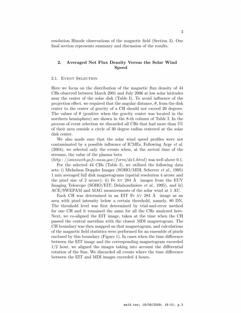
Each CH was determined in an EIT Fe xv 284 A image as anarea with pixel intensity below a certain threshold, namely, 80 DN.The threshold level was first determined by trial-and-error methodfor one CH and it remained the same for all the CHs analyzed here.Next, we co-aligned the EIT image, taken at the time when the CHpassed the central meridian with the closest MDI magnetogram. TheCH boundary was then mapped on that magnetogram, and calculationsof the magnetic field statistics were performed for an ensemble of pixelsenclosed by this boundary (Figure 1). In cases when the time differencebetween the EIT image and the corresponding magnetogram exceeded1/2 hour, we aligned the images taking into account the differentialrotation of the Sun. We discarded all events where the time differencebetween the EIT and MDI images exceeded 4 hours.

ms14.tex; 18/08/2009; 18:01; p.3

4

One more criteria was used to ensure that a given CH is indeedassociated with the feature observed in the solar wind speed profile. Incase of the positive association, the polarity of the Bx component ofthe solar wind magnetic field, measured in the GSE coordinate systemby ACE/MAG, should be opposite to that of the open flux in the baseof the CH because the x-axis in the GSE system points from the Earthtoward the Sun, while the positive magnetic field on the solar surfaceis directed outward from the Sun. Only those CHs, for which magneticpolarities satisfied the above condition, were included into this study.

Figure 1. SOHO/MDI magnetogram (left) and the corresponding SOHO/EIT 284Aimage taken at 19:06 UT on 2 March 2002 (right). The contour indicates theboundary of coronal hole CH201 (see Table I).

2.2. Solar Wind Speed Derivation

For each CH in our data set, we determined the solar wind speed, Vx.We utilized the 64 s averaged time profiles measured in the GSE coor-dinate system with ACE/SWEPAM instruments. Note that the solarwind speed acquires negative values in the GSE coordinate system.

The arrival time at 1 AU of the solar wind associated with the CHwas determined as the moment t, when a function

∆r(t) = Vx(t − t0) − 1AU (1)

turns into zero. Here, t0 (3rd column of Table I) is the CH culminationtime, and t = tA (4-th column of Table I) is the arrival time.

We then accepted that the association between the CH and thesolar wind feature is reliable when tA, calculated from Equation (1),falls into the well pronounced “dip” in the observed solar wind speed

ms14.tex; 18/08/2009; 18:01; p.4

5

profile. Figure 2 shows an observed time profile of the solar wind speedand the corresponding profile of ∆r(t) associated with the CH shownin Figure 1.

60 62 64 66

CH201 2002 Mar 02

60 62 64 66Day of year 2002

-900

-800

-700

-600

-500

-400

-300

SW

spe

ed, v

x(A

CE

) ,

km s

-1

<vx>= -649 + - 28

to tA

Figure 2. Observed time profile of the Vx component of the solar wind speed (redcurve) as measured by ACE satellite from 0000UT on 28 February 2002 until 2359UTon 7 March 2002. The black curve represents a smoothed over 21-point observedspeed profile. The vertical dotted line indicates the CH culmination time, t0, whilethe vertical solid line indicates the solar wind arrival time, tA. The arrival time wasdetermined as the moment when parameter ∆r (double green curve) is equal to zero.The blue thick horizontal line segment shows the time interval used to determine theaverage, for a given event, solar wind speed, 〈Vx〉 (indicated by the vertical positionof the blue line segment).

The magnitude of the solar wind speed, 〈Vx〉, was determined byaveraging the observed time profile of Vx(t) over a time interval thatincludes the minimum of the observed speed profile. This time interval(marked by the thick blue horizontal segment in Figure 2) was definedin the following way. First, we applied a 21-point running averaging tothe observed Vx(t) profile (red curve in Figure 2). This smoothed profile(black curve) was then used to determine i) the level of undisturbedslow-wind speed, V0, preceding the CH, and ii) the maximum speedinside the CH, Vmax. To obtain the averaged solar wind speed, 〈Vx〉,

ms14.tex; 18/08/2009; 18:01; p.5

6

we averaged all data points inside an interval where Vx(t) is lower thanVmax +(|Vmax|− |V0|)/4. This threshold was chosen by a trial-and-errormethod. The resulting averaged solar wind speed is indicated in Figure2 by the vertical position of the blue line segment. We would like toemphasize here that we did not include in our study those CHs whoseassociated speed profile was so complex that no well defined minimumcould be chosen.

For each CH in our data set, the area of the CH (in pixels of theMDI full disk magnetogram) and the associated solar wind speed arelisted in the 7-th and 9-th columns of Table I, respectively.

The above routine allowed us to determine the arrival time and themagnitude of the solar wind speed individually for each coronal hole.This technique differs from that applied by Robbins et al. (2006) andVrsnak et al. (2007), where the mean arrival time, determined from thecross-correlation technique, was utilized.

2.3. Magnetic Parameters

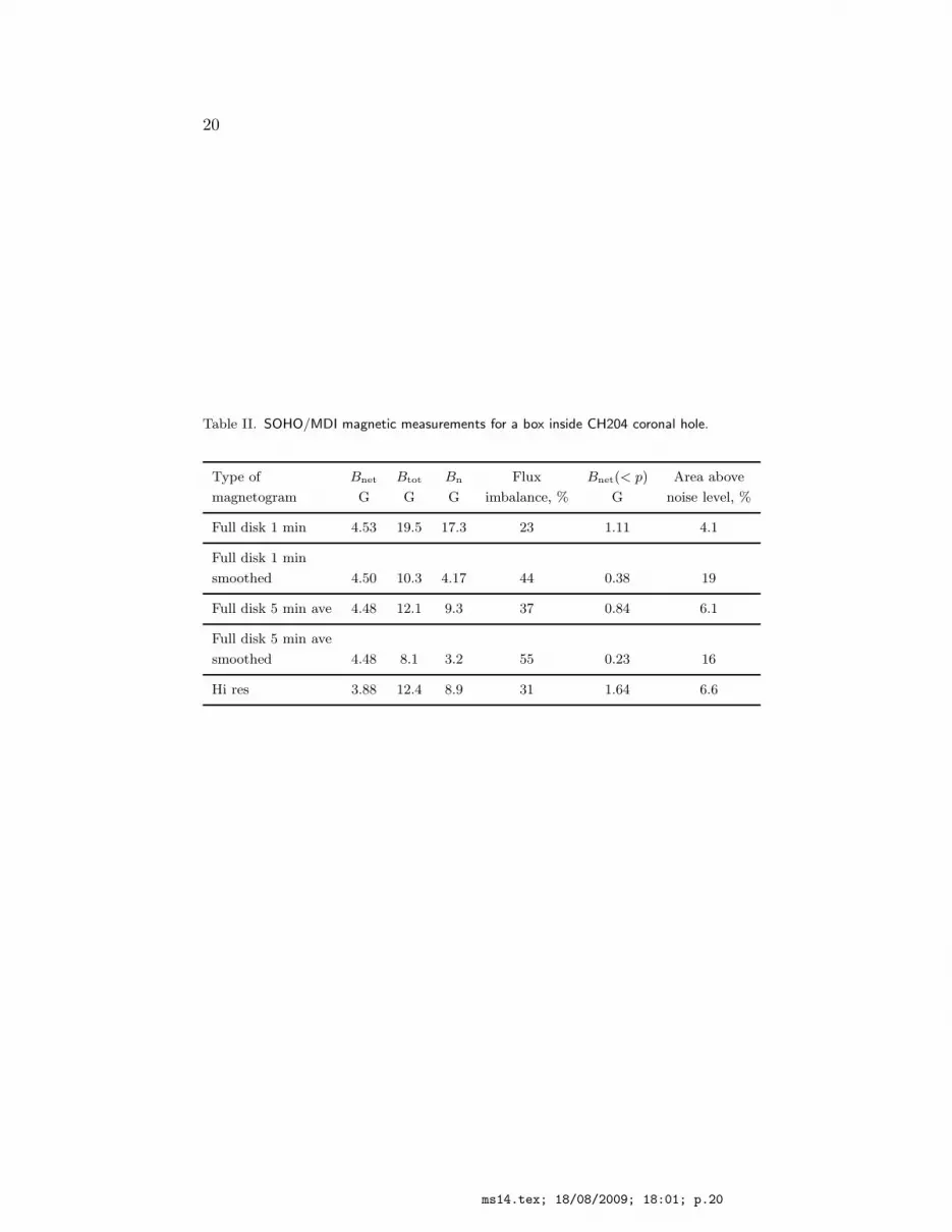
The above selection routine left us with a set of 44 CHs. MDI fulldisk 1 minute average magnetograms were available for all of them.However, the full disk data of 1 minute cadence, as well as the obser-vations in the MDI high resolution mode, were not available for all ofthem. Since we are interested in measurements of the net magnetic fluxdensity, we decided first to focus on whether the measurements of thisparameter from 1 minute full disk magnetograms are reliable. To dothat, we analyzed coronal hole CH 204 from our data list (see TableI), for which nearly simultaneous observations in two MDI modes wereavailable: 1 minute cadence full disk and high resolution modes. Insidethis large coronal hole, located at the solar disk center, we outlined arectangular area of n × m pixels and calculated magnetic parametersfor five different magnetograms. Results are compiled in Table II, wherethe first row is the result from one original individual MDI full disk 1minute magnetogram. The second row represents results from the samemagnetogram, but smoothed in both directions with a boxcar averageof three pixels. The third row are parameters from a magnetogramderived from averaging of five consecutive original 1 min magnetograms,whereas its smoothed version is presented in the next row. The last rowrepresents results from the high resolution MDI magnetogram recordedat the same place on the Sun with pixel size of 0.6 arcsec.

From each of the above magnetograms, we first calculated the netflux density, Bnet =

∑B||/(n×m) (2nd column in Table II), inside the

box. We note that the net flux is obtained by summing all pixel valueswith their sign. This procedure results in cancellation of the bulk of

ms14.tex; 18/08/2009; 18:01; p.6

7

sign-variable noise. Magnetic flux confined in loops, closed within theCH, will also be canceled. This allowed us to assume that in CHs, thenet flux density also represents the open magnetic flux density.

The density of the total unsigned flux, Btot =∑

|B|||/(n × m),is shown in the 3rd column of Table II. The 4-th column representsthe density, Bn, of the noise in magnetograms derived from the powerspectrum calculations as it was suggested by Longcope and Parnell(2008). To derive this parameter, we calculated a 1D power spectrum,S(k), from each magnetogram and then calculated the noise density asBn = (πk2

cS(kc))1/2, where kc = 2π1/2∆x is the maximum wave num-

ber. The imbalance of the magnetic flux is shown in the 5-th column.The 6-th column represents the density of the net flux calculated overthe area where |B||| < 3Bn (we denote 3Bn = p), and the last columnshows the fraction of the box area, where the flux density exceeds thetriple noise level, |B||| > p.

Data of Table II indicate that the density of the net flux, Bnet, doesnot vary much (by less than 2%) with temporal/spatial averaging anddoes not depend on the noise level. At the same time, the density ofthe unsigned flux, Btot, depends significantly on the noise level. (Notethat the magnitude of Bn is in good agreement with the results fromMDI full disk data noise reduction reported by Hagenaar et al. (2008)).Last two columns in Table II show that the bulk of the magnetic fluxin CHs is concentrated within a small (a few percents) fraction of theCH’s area. Vast zones of low fluctuations contribute only about 1 Ginto the resulting magnitude (4 G) of the net flux density.

This experiment shows, first, that an averaging procedure is undesir-able when one intends to analyze fine structures of the magnetic field.Second, that the net flux density in coronal holes is measured with thesame level of confidence from the original and averaged magnetograms.High noise level in original magnetograms does not influence much onthe Bnet calculations. The reasons for that are: i) high imbalance of themagnetic flux inside coronal holes, accompanied by low (as compared toadjacent quiet sun areas) rate of dipole emergence (Abramenko et al.,2006; Hagenaar et al., 2008); and ii) magnetic features that contributeto the open flux are predominantly well above the noise level, even forthe noisiest magnetogram.

For 44 coronal holes analyzed here, magnitudes of the net magneticflux, Φnet =

∑B||∆s, where ∆s is a pixel size, are presented in the

5-th column of Table I. The 6-th column shows the densities of the netmagnetic flux, Bnet =

∑B||/A, where A is the area in pixels inside the

CH boundary, 7-th column in Table I. We would like to emphasize thatthe moduli of Bnet tend to decrease from March 2001 toward July 2006,

ms14.tex; 18/08/2009; 18:01; p.7

8

i.e., toward the end of the 23rd cycle. This is in qualitative agreementwith Harvey et al. (1982).

2.4. Correlations Between Calculated Parameters

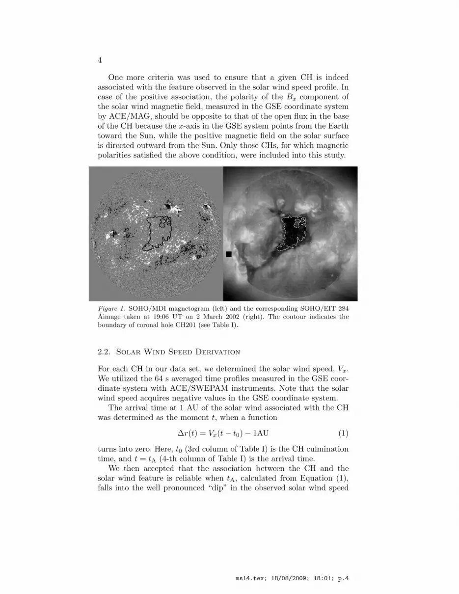
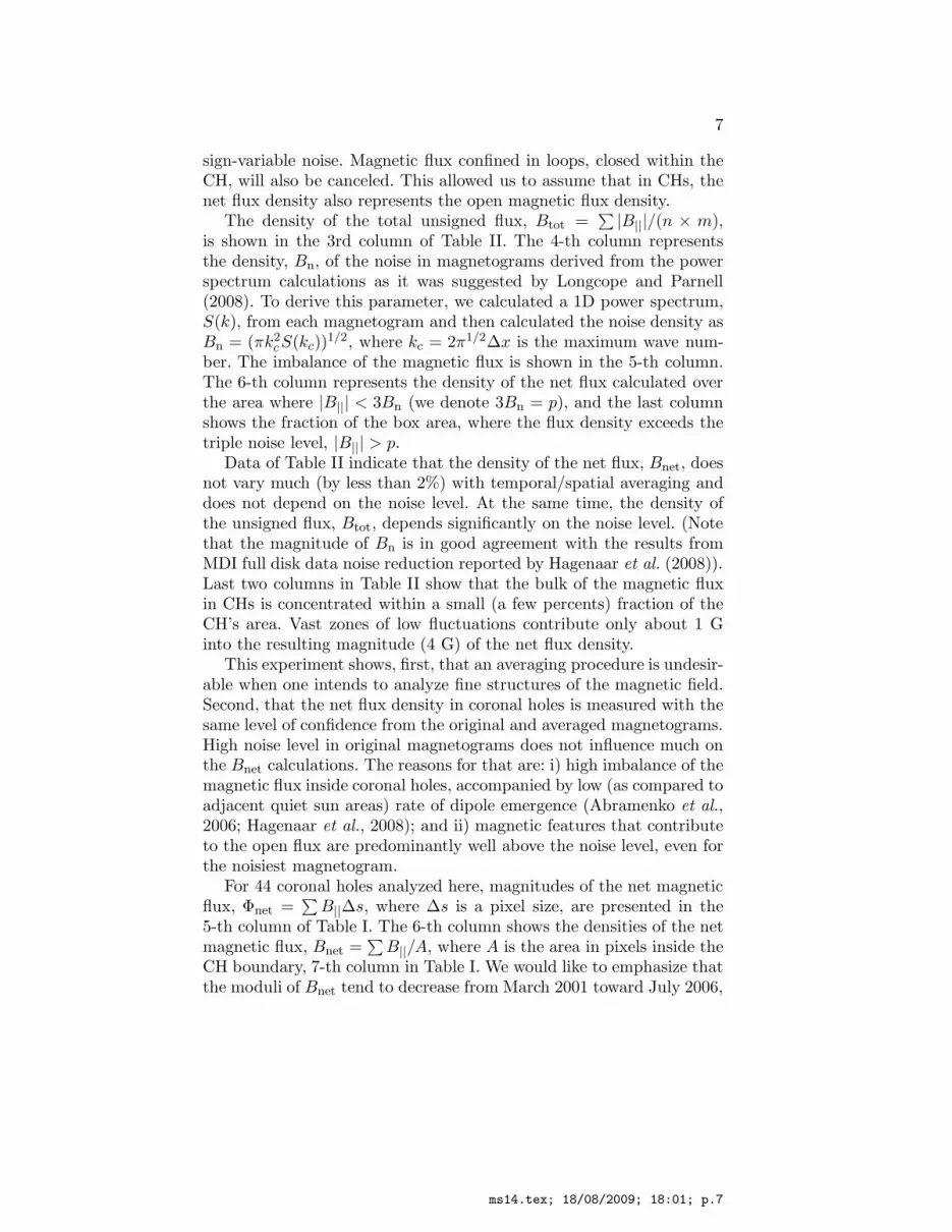
Figure 3 shows correlations between parameters of CHs and the solarwind speed. The solar wind speed, 〈Vx〉, is directly correlated with thetotal net flux (upper left panel). The corresponding Pearson coefficientis 0.71 and the linear fit is given by

〈Vx〉 = 494 + 47.4 · Φnet, (2)

where 〈Vx〉 is in km s−1 and Φnet is in 1021 Mx.However, the total net flux is a product of the CH area, A, and the

average net flux density, Bnet. According to Figure 3, the solar windspeed is strongly correlated with the CH area (upper right panel, corre-lation coefficient (cc)=0.75) and only weekly depends on the averagednet flux density (lower left panel, cc=0.20). Linear fitting to the datapoint gave us the following relationship between the speeds and CHareas:

〈Vx〉 = 486 + 8.50 · A, (3)

where A is in 104 arcsec2. As a result, there is a very strong dependenceof the total net magnetic flux from the CH area (cc=0.92, lower rightpanel), which allows a reliable estimation of the total open flux in aCH:

Φnet = 0.045 + 0.156 · A, (4)

where Φnet is in 1021 Mx and A is in 104 arcsec2.These findings very well agree with previously reported results (Wang

and Sheeley, 1990; Robbins et al., 2006; Vrsnak et al., 2007; Schwadronand McComas, 2008) in spite of differences in used techniques. Thisconsistency indicates reliability of the coronal hole analysis presentedhere.

On many occasions, analyzed CHs had closed loop structures embed-ded within them, which, in general, reduces the area occupied by theopen flux and may lead to different magnitudes of the averaged totalflux density. We excluded the closed loop areas from our calculationsand repeated the above analysis. As expected, since the closed loopregions substitute a small fraction of the CH area, accounting for themdid not lead to a significant change of the relationship between the solarwind speed and the total flux density. In fact, the Pearson coefficienteven slightly decreased to 0.15.

We finally would like to note that the well defined relationship be-tween the speed and area opens up a possibility to estimate the solar

ms14.tex; 18/08/2009; 18:01; p.8

9

wind speed 3-4 days in advance by measuring the area of a CH, whenit passes the central meridian. (Note that in this study the CH areawas measured inside a contour of 80 DN in EIT/Fe xv 284 A images.)

0 10 20 30 40Area, 104 arcsec2

200

400

600

800

Vx,

km

s-1

CC = 0.750

0 10 20 30 40 50Area, 104 arcsec2

0

2

4

6

8|Φ

net|,

1021

Mx

CC = 0.916

0 2 4 6 8Bnet, G

200

400

600

800

Vx,

km

s-1

CC = 0.195

0 2 4 6|Φnet|,1021 Mx

200

400

600

800

Vx,

km

s-1

CC = 0.711

Figure 3. Correlations between magnetic parameters of coronal holes and solar windparameters. Solid straight lines represent the best linear fit to the data points.

3. Multifractality in the Magnetic Field in Coronal Holes

The absence of a relationship between the solar wind speed and thedensity of the magnetic flux, seems to be suspicious at the first sight.The solar wind speed represents the intensity of the solar wind ac-celeration processes, i.e., energy release dynamics, which ultimately isrelated to the magnetic field. Numerous recent studies of the dynamicsof energy release in the low corona based on Hinode data (Baker et al.,2008; Suematsu, 2008; Shimojo, 2008; Moreno-Insertis et al., 2008) tell

ms14.tex; 18/08/2009; 18:01; p.9

10

us that there is a role for the magnetic field to play in these phenomena.Two things could be done to resolve the problem. First, improve spatialresolution of magnetic field measurements, and second, explore theproper measures of complexity of the magnetic field.

The Solar Optical Telescope (SOT, Tsuneta et al., 2008) onboardHinode has a 50 cm aperture mirror and is the largest optical solartelescope ever sent to space. The Hinode/Spectropolarimeter (SP, Ichi-moto et al., 2008) obtains the full Stokes parameters using the Fei 630 nm absorption line and offers a unique opportunity to obtainmagnetograms with pixel size of 0.32 arcsec in the fast mode and0.16 arcsec in the normal mode. Coronal holes at low latitudes arerare during a solar minimum, where we are now. Nevertheless, on 11November 2008 the SOT/SP instrument recorded a CH (Figure 4) atthe disk center in the fast mode. We analyzed here one of the SOT/SPmagnetograms of 942×500 pixels taken in the fast mode (Figure 5). Theinversion code and calibration routine were performed at HAO CSAC(http : //www.csac.hao.ucar.edu/). The magnetogram was carefullydespiked.

It is believed now that magnetic structures in active regions and inquiet sun areas are fractals (Tarbell et al., 1990; Schrijver et al., 1992;Balke et al., 1993; Lawrence et al., 1993; Meunier, 1999; Ireland et al.,2004; Janssen et al., 2003; McAteer et al., 2005). In particular, Meunier(1999) and McAteer et al. (2005) showed that magnetic structures ofactive regions, even those recorded with 4 arcsec resolution (MDI fulldisk magnetograms), are fractals. Janssen et al. (2003) showed thatthe magnetic field in a quiet sun ares is also a fractal. Fractals areself-similar, porous structures with jagged boundaries. Their scalingparameters do not vary with spatial scale. For example, the fillingfactor, i.e., the ratio of the area occupied by (above-noise) fields to theentire area, does not vary when the resolution changes. An example: acomparison of the 3rd and 5-th rows in the last column in Table II tellus that the fraction of the area occupied by strong fields is nearly thesame, about 6%, for the 4 arcsec and 1.2 arcsec resolutions. This mightindicate that the coronal hole magnetic field structure at these scalescan be considered as a single fractal, or, in other words, a monofractal.

Temporal variations in monofractal structures are non-intermittent,i.e., high fluctuations in energy release are very rare and they do notrepresent a burst-like behavior. Therefore, strong energy release eventsare rare and they do not define the energy balance dynamics.

Another situation is when a multifractal is formed. Multifractalsform in nature ubiquitously when several processes contemporaneouslygovern formation of a structure, each one dictating its own rules ofclustering and fragmentation. A highly intermittent temporal behavior

ms14.tex; 18/08/2009; 18:01; p.10

11

is inherent for multifractals, so that high fluctuations in energy releaseare not rare, and the regime of violent, burst-like energy release dy-namics is set. Therefore, to relate the energy release dynamics withthe magnetic field, one should find the spatial scales where multifractalproperties of the magnetic field manifest themselves, if any. (Note thatthe terms multifractality and intermittency describe the same propertyof a structure. However, the former is related to the spatial domainwhile the later is usually utilized for the temporal domain; see, e.g.,Abramenko (2008) for details.)

One of possible ways to diagnose multifractality is based on calcu-lation of the filling factor as a function of spatial scale (Frisch, 1995).For multifractals, the filling factor decreases as the scale decreases. Inother words, the fraction of a volume occupied by strong fields (the socalled active mode), decreases as we study the multifractal at smallerand smaller scales. For monofractals, this ratio is constant with scale.To this end, our goal was to explore how the filling factor varies withscale inside coronal holes.

The ratio of the active mode to the entire volume as a function ofthe scale, r, can be calculated from the flatness function, which for thelongitudinal magnetic field Bl, can be written as (Frisch, 1995):

F (r) = S4(r)/(S2(r))2. (5)

Here,Sq(r) = 〈|Bl(x + r) − Bl(x)|q〉 (6)

are the structure functions, and x is the current pixel on a magne-togram, r is the separation vector (i.e., the spatial scale), and q isthe order of a statistical moment, which takes on real values. Theangular brackets denote averaging over the magnetogram. Details ofthe calculation routines and applications can be found in Abramenkoet al. (2002, 2003, 2008) and in Abramenko (2005). The filling factoris then calculated as

f(r) = 1/F (r). (7)

As it was mentioned above, the filling factor does not depend on thespatial scale, r, in case of a monofractal structure. On the contrary, fora multifractal, the filling factor displays a power-law decrease as thescales become progressively smaller.

Results of the filling factor are presented in Figure 6. Hinode/SOT/SPdata for the CH observed on 30 November 2008 (blue curve) indicatesthat at scales larger than approximately 2 Mm, the magnetic fieldstructure seems to be a monofractal. Only a very slight slope (0.024) ofthe power law linear fit is observed. Thus, at scales larger than 2 Mm,the magnetic field in a coronal hole seems to be a monofractal.

ms14.tex; 18/08/2009; 18:01; p.11

12

Figure 4. The 11:42UT XRT image on 30 November 2008. The box in the cen-ter of the solar disk outlines the area inside a coronal hole where the SOT/SPmagnetogram was taken (Figure 5).

For comparison, we calculated and plotted in the same graph (Figure6) the filling factor for an active region NOAA 0930 and a plage areato the west of this active region. The corresponding magnetogramswere also derived with the SOT/SP instrument in the fast mode andprocessed with the same routines as those applied for the CH magne-togram. Data for the AR and plage show a steeper slope of the powerlaw linear fit with indices of 0.18 and 0.09, respectively. The dependenceof the filling factor on the scale implies multifractality of the magneticfield at scales larger than 2 Mm.

To double check our inference on monofractality in CHs at largescales, we calculated the filling factor from the MDI/HR data for 36square areas located inside 19 coronal holes observed during 2002-2004at the solar disk center. The MDI results are shown in Figure 6 with the

ms14.tex; 18/08/2009; 18:01; p.12

13

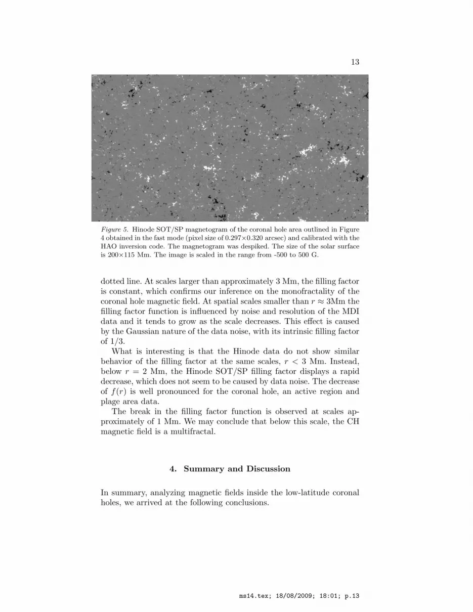
Figure 5. Hinode SOT/SP magnetogram of the coronal hole area outlined in Figure4 obtained in the fast mode (pixel size of 0.297×0.320 arcsec) and calibrated with theHAO inversion code. The magnetogram was despiked. The size of the solar surfaceis 200×115 Mm. The image is scaled in the range from -500 to 500 G.

dotted line. At scales larger than approximately 3 Mm, the filling factoris constant, which confirms our inference on the monofractality of thecoronal hole magnetic field. At spatial scales smaller than r ≈ 3Mm thefilling factor function is influenced by noise and resolution of the MDIdata and it tends to grow as the scale decreases. This effect is causedby the Gaussian nature of the data noise, with its intrinsic filling factorof 1/3.

What is interesting is that the Hinode data do not show similarbehavior of the filling factor at the same scales, r < 3 Mm. Instead,below r = 2 Mm, the Hinode SOT/SP filling factor displays a rapiddecrease, which does not seem to be caused by data noise. The decreaseof f(r) is well pronounced for the coronal hole, an active region andplage area data.

The break in the filling factor function is observed at scales ap-proximately of 1 Mm. We may conclude that below this scale, the CHmagnetic field is a multifractal.

4. Summary and Discussion

In summary, analyzing magnetic fields inside the low-latitude coronalholes, we arrived at the following conclusions.

ms14.tex; 18/08/2009; 18:01; p.13

14

Figure 6. Variation of the filling factor, f , with spatial scale, r. Blue - data from theHinode/SOT/SP magnetogram of the coronal hole shown in Figure 5. Black dots- the averaged filling factor calculated from 36 magnetograms for 19 coronal holesobserved between 2002 and 2004 with SOHO/MDI in the high resolution mode.The flat filling factor is observed at scales above 3 Mm in both data sets. Thedecreasing of the filling factor at scales below 2 Mm is observed in SOT/SP data.For comparison, data for the active region NOAA 0930 (red) and weak plage area(green) derived from the Hinode/SOT/SP fast mode magnetograms are shown. Theactive region and the plage area display the decreasing filling factor at large scalesabove 2 Mm. Dashed lines represent the best linear fit to the data points inside aninterval of ∆r = (1.6 − 8.2) Mm. The steeper slope of the fit corresponds to higherdegree of multufractality.

i) The density of the net magnetic flux does not correlate with thecorresponding in situ solar wind speeds. At the same time, both CHarea and total net flux correlate very well with the solar wind speed andthe corresponding spatial Pearson correlation coefficients determined

ms14.tex; 18/08/2009; 18:01; p.14

15

for 44 CHs are 0.75 and 0.71, respectively. The relationship betweenthe CH areas and the solar wind speed with almost the same results incorrelation was earlier derived by Robbins et al. (2006) and by Vrsnaket al. (2007).

As we discussed in Section 1, the fact that the net magnetic fluxdensity is not correlated with the solar wind speed can hardly beinterpreted as irrelevance of the magnetic field to the solar wind ac-celeration process. One would rather suggest that the net flux densitymeasured with the resolution of 4 arcsec does not reflect the energyrelease dynamics inside CHs. Analysis of SOHO/MDI/high-resolutionand Hinode/SOT/SP magnetograms seems to support this suggestion.

ii) The filling factor as a measure of multifractality in CHs was cal-culated as a function of spatial scale. It was found to be nearly constantat scales above 2 Mm. Its magnitude is approximately 0.04 from theHinode data and 0.07 from the MDI/HR data. At scales smaller than2 Mm, the filling factor starts to decline as the scale becomes smaller,and at approximately 1 Mm the regime of fast decrease of the fillingfactor is set.

A constant filling factor at r > 2 Mm in the CH magnetic fields indi-cates their monofractal nature and self-similarity. A self-similar struc-ture by definition possesses constant statistical parameters at all scales(such as various scaling exponents, including the filling factor). How-ever, only for artificial, mathematically created fractals, self-similarityis present at infinite range of scales (see, e.g., Schroeder, 1991). Fora majority of structures in nature, however, self-similarity with con-stant scaling parameters only holds at a finite range of scales, whileat the entire interval of scales the scaling parameters are different. Asa result, a multifractal structure forms with a superposition of manyfractals, each one imposing its own scaling rules. A crucial differencebetween monofractals and multifractals is in their temporal evolution.In monofractals, large fluctuations of parameters (say, energy releaseevents) are rare and do not determine mean values. In other words, timeprofiles are non-intermittent and evolution proceeds without catastro-phes. On the contrary, in multifractals, the time profiles are highlyintermittent, large fluctuations are not rare, and they determine meanvalues. The temporal energy release process is burst-like.

If so, the monofractal property of the CH magnetic field at scalesabove 2 Mm seems to be the most plausible reason why the averagedmagnetic flux density, derived from observations with low resolution,does not correlate with the solar wind speed: the bulk of energy releasedynamics, needed for the solar wind acceleration, occurs at smallerscales, where the magnetic field structure is entirely different.

ms14.tex; 18/08/2009; 18:01; p.15

16

Berger and colleagues (Berger et al., 2004) observed a plage areawith 0.1 arcsec resolution, and they report that the magnetic flux isstructured into amorphous ribbon-like clusters with embedded knotsof enhanced density, which seems to correspond to the notion of mul-tifractality at small scales.

It is worth to mention that the property of monofractality of solarmagnetic fields was known for a long time (see references in the previoussection). Difficulties of describing magnetic structures with a singlefractal dimension at the entire range of scales was also noticed (see, e.g.,Tarbell et al., 1990; Janssen et al., 2003), which actually is a signature ofmultifractality. Fractal analysis of high resolution magnetograms fromVTT with 0.4 arcsec spatial resolution for a quiet sun area (Janssen et

al., 2003) revealed a break of self-similarity at scales of 1.3 Mm, whichis very close to the scale found in this study.

For an active region and a plage area, our approach for deriving thefilling factor of the magnetic field produced that f(r) = 0.14 − 0.17at r = 0.3 Mm that generally agree with earlier reports. According toTarbell et al. (1979), Schrijver (1987), Berger et al. (1995) and refer-ences herein, the magnetic filling factor is typically inside a range of 10- 25%. In active regions, where the range of solar flares spreads over allobservable scales, multifractality is also present at the same range ofscales. This presents further evidence that energy release dynamics andthe multifractality are mutually related properties of solar magneticfields.

With the Hinode instrument in operation, many new phenomenarelated to the CH dynamics, coronal heating and solar wind acceler-ation will be discovered now, when the spatial scales less than 1000km are available for analysis. Recent study of the evolution of networkmagnetic elements (Lamb et al., 2008) proved that processes at sub-resolution scales are of vital importance for understanding the observeddynamics of magnetic flux.

Acknowledgements. Authors thank Spiro Antiochos, Len Fisk, Den-nis Haggerty, Marco Velli, Yi-Ming Wang, Thomas Zurbuchen and theentire LWS/TR&T Heliospheric Focus Team for helpful discussionsand initiation of this research. We also thank Rob Markel for valu-able assistance in during the inversion process, and anonymous refereeswhose criticism and comments led to a significant improvement of themanuscript. We thank the ACE MAG and SWEPAM instrument teamsand the ACE Science Center for providing the ACE data. SOHO is aproject of international cooperation between ESA and NASA. Hinodeis a Japanese mission developed and launched by ISAS/JAXA, col-laborating with NAOJ as a domestic partner, NASA and STFC (UK)as international partners. Scientific operation of the Hinode mission is

ms14.tex; 18/08/2009; 18:01; p.16

17

conducted by the Hinode science team organized at ISAS/JAXA. Thisteam mainly consists of scientists from institutes in the partner coun-tries. Support for the post-launch operation is provided by JAXA andNAOJ (Japan), STFC (U.K.), NASA (U.S.A.), ESA, and NSC (Nor-way). Hinode SOT/SP inversions were conducted at NCAR under theframework of the Community Spectro-polarimtetric Analysis Center(CSAC; http : //www.csac.hao.ucar.edu/). This work was supportedby NASA NNX07AT16G grant, and NSF grant ATM-0716512.

References

Abramenko, V.I.: 2005, Solar Phys. 228, 29.Abramenko, V.I.: 2008, In: Wang, P.(ed), Solar Physics Research Trends, Nova

Science Publishers, Inc., New York, 95.Abramenko, V.I., Yurchyshyn, V.B., Wang, H., Spirock, T.J., Goode, P. R.: 2002,

Astrophys. J. 577, 487.Abramenko, V.I., Yurchyshyn, V.B., Wang, H., Spirock, T.J., Goode, P. R.: 2003,

Astrophys. J. 597, 1135.Abramenko, V. I., Fisk, L. A., Yurchyshyn, V. B.: 2006, Astrophys. J. 641, L65.Abramenko, V.I., Yurchyshyn, V.B., Wang, H.: 2008, Astrophys. J. 681, 1669.Arge, C.N., Luhmann, J.G., Odstrcil, D., Schrijver, C.J., Li, Y.: 2004, J. Atmos.

Solar Terr. Phys. 66, 1295.Baker, D., van Driel-Gesztelyi, L., Kamio, S., Culhane, J. L., Harra, L.K., Sun, J.,

Young, P.R., Matthews, S.A.: 2008, In: Matthews, S.A., Davis, J.M., Harra, L.K.(eds), First Results From Hinode, ASP Conf. Ser. 397, 23.

Balke, A.C., Schrijver, C.J., Zwaan, C., Tarbell, T.D.: 1993, Solar Phys. 143, 215.Berger, T.E., Schrijver, C.J., Shine, R.A., Tarbell, T.D., Title, A.M., Scharmer, G.:

1995, Astrophys. J. 454, 531.Berger, T. E., Rouppe van der Voort, L. H. M., Lofdahl, M. G., Carlsson, M.,

Fossum, A., Hansteen, V. H., Marthinussen, E., Title, A., Scharmer, G.: 2004,Astron. Astrophys. 428, 613.

Bumba, V., Klvana, M., Sykora, J.: 1995, Astron. Astrophys. 298, 923.Delaboudiniere, J.-P., Artzner, G.E., Brunaud,J., Gabriel, A.H.,Hochedez, J.F.,

Millier, F., ⁀ei al.: 1995, Solar Physics 162, 291.Fisk, L.A.: 1996, J. Geophys. Res. 101, 15547.Fisk, L.A.: 2001, J. Geophys. Res. 106, 15849.Fisk, L.A.: 2005, Astrophys. J. 626, 563.Fisk, L.A., Zurbuchen, T. H., Schwadron, N.A.: 1999, Astrophys. J. 521, 868.Frisch, U.: 1995, Turbulence, The Legacy of A.N. Kolmogorov, Cambridge University

Press, Cambridge, 296.Hagenaar, H. J., DeRosa, M. L., Schrijver, C. J.: 2008, Astrophys. J. 678, 541.Harvey, J., Krieger, A. S., Timothy, A. F., Vaiana, G. S.: 1975, Oss. Mem. Oss.

Arcetri 104, 50.Harvey, J. W., Sheeley, N. R., Jr.: 1979, Space Sci. Rev. 23, 139.Harvey, K. L., Harvey, J. W., Sheeley, N. R., Jr.: 1982 Solar Phys. 79, 149.Ichimoto, K., Lites, B., Elmore, D., Suematsu, Y., Tsuneta, S., Katsukawa, Y., et

al.: 2008, Solar Phys. 249, 233.

ms14.tex; 18/08/2009; 18:01; p.17

18

Ireland, J., Gallagher, P.T., McAteer, R.T.J.: 2004, In: Dupree, A.K., Benz, A.O.(eds), Stars as Suns: Activity, Evolution and Planets, IAU Symp. 219, 255.

Janssen, K., Vogler, A., Kneer, F.: 2003, Astron. Astrophys. 409, 1127.Lamb, D. A., DeForest, C. E., Hagenaar, H. J., Parnell, C. E., Welsch, B. T.: 2008,

Astrophys. J. 674, 520.Kamio, S., Hara, H., Watanabe, T., Matsuzaki, K., Shibata, K., Culhane, L., Warren,

H.P.: 2007, Publ. Astron. Soc. Japan 59, S757.Lawrence, J.K., Ruzmaikin, A.A., Cadavid, A.C.: 1993, Astrophys. J. 417, 805.Longcope, D.W., Parnell, C.E.: 2008, Solar Physics 254, 51.McAteer, R.T.J., Gallagher, P.T., Ireland, J.: 2005, Astrophys. J. 631.Meunier, N.: 1999, Astrophys. J. 515, 801.Moreno-Insertis, F., Galsgaard, K., Ugarte-Urra, I.: 2008, Astrophys. J. 673, L211.Obridko, V. N., Shelting, B. D.: 1989, Solar Phys. 124, 73.Obridko, V., Formichev, V., Kharshiladze, A. F., Zhitnik, I., Slemzin, V., Hathaway,

D., Wu, S. T.: 2000, Astron. Astrophys. Trans. 18, 819.Robbins, S., Henney, C. J., Harvey, J. W.: 2006, Solar Phys. 233, 265.Scherrer, P.H., Bogart, R.S., Bush, R.I., Hoeksema, J.T., Kosovichev, A.G., Schou,

J., et al.: 1995, Solar Phys. 162, 129.Schrijver, C.J.: 1987, Astron. Astrophys. 180, 241.Schrijver, C.J.: 2001, Astrophys. J. 547, 475.Schrijver, C.J., Zwaan, C., Balke, A.C., Tarbell, T.D., Lawrence, J.K.: 1992, Astron.

Astrophys. 253, L1.Schrijver, C.J., Title, A.M.: 2001, Astrophys. J. 551, 1099.Schrijver, C.J., DeRosa, M.L., Title, A.M.: 2002, Astrophys. J. 577, 1006.Schrijver, C.J., DeRosa, M.L.: 2003, Solar Phys. 212, 165.Schroeder, M.: 1991, Fractals, Chaos, Power Laws, W.H. Freeman and Company,

New York, 429.Schwadron, N.A., McComas, D.J.: 2008, AGU, Fall Meeting, SH13B-1559.Sheeley, N.R., Jr., Harvey, J.W., Feldman, W.C.: 1976, Solar Phys. 49, 271.Shimojo, M.: 2008, AGU, Fall Meeting, SH22A-0836.Suematsu, Y.: 2008, AGU, Fall Meeting, SH41B-1623.Tarbell, T.D., Title, A.M., Schoolman, S.A.: 1979, Astrophys. J. 229, 387.Tarbell, T., Ferguson, S., Frank, Z., Shine, R., Title, A., Topka, K., Scharmer,

G.: 1990, In: Stenflo, J.O. (ed.), Solar Photosphere: Structure, Convection, and

Magnetic fields, IAU Symp. 138, 147.Tsuneta, S., Ichimoto, K., Katsukawa, Y., Nagata, S., Otsubo, M., Shimizu, T., et

al.: 2008, Solar Phys. 249, 167.Vrsnak, B., Temmer, M., Veronig, A.M.: 2007, Solar Phys. 240, 315.Wang, Y.M., Sheeley, N.R.: 1990, Astrophys. J. 355, 726.Wang, Y.M., Sheeley, N.R.: 1991, Astrophys. J. 375, 761.Wang, Y.M., Lean, J., Sheeley, N.R.: 2000, Geophys. Res. Lett. 27, 505.Wiegelmann, T., Solanki, S.K.: 2004, Solar Phys. 225, 227.Wiegelmann, T., Xia, L. D., Marsch, E.: 2005, Astron. Astrophys. 432, L1.

ms14.tex; 18/08/2009; 18:01; p.18

19

Table I. List of studied coronal holes and the corresponding parameters.

CH Culmination t0, tA, Φnet, Bnet A, θ, 〈Vx〉,

name time doy doy 1021 Mx G pixels deg km s−1

CH191 2001Mar02/23:00 61.96 64.96 3.00 5.01 29145 17.2 559 ±16

CH230 2002Feb03/22:00 34.92 37.75 1.09 3.43 15408 -2.8 614 ±27

CH201 2002Mar02/17:00 61.71 64.38 3.03 4.27 34472 2.2 649 ±28

CH202 2002Mar29/18:00 88.75 91.08 2.61 4.22 30127 1.7 701 ±38

CH210 2002Apr28/23:00 118.96 122.63 0.84 3.85 10621 -19.6 462 ±14

CH231 2002Jul03/12:00 184.5 187.67 -0.92 -4.60 9721 -13.2 536 ±16

CH204 2002Nov01/17:00 305.71 309.04 1.49 2.54 28578 -6.3 549 ±16

CH350 2003Jan27/06:00 27.25 30.67 -0.24 -4.75 2555 1.6 507 ±14

CH302 2003Feb23/19:00 54.79 58.13 -2.04 -4.26 23176 7.1 560 ±18

CH303 2003Mar01/03:00 60.13 63.29 -1.65 -4.76 16856 14.2 530 ±32

CH304 2003Apr08/09:00 98.38 100.79 3.12 2.73 55633 -7.9 702 ±27

CH305 2003Apr24/07:00 114.29 117.71 -0.29 -2.67 5407 0.2 510 ±23

CH307 2003May03/19:00 123.79 126.38 3.07 3.23 46245 -11.1 693 ±23

CH354 2003May21/01:00 141.04 144.54 -1.43 -3.12 22381 -1.0 530 ±31

CH309 2003May25/19:00 145.79 148.21 -0.93 -5.59 8151 -20 701 ±31

CH312 2003Jun11/11:00 162.46 165.63 -0.47 -2.51 9260 -0.6 548 ±21

CH355 2003Aug10/01:00 222.04 224.63 -2.61 -2.43 52146 3.6 650 ±25

CH314 2003Aug20/19:00 232.79 235.04 4.57 2.66 83592 -4.9 741 ±28

CH356 2003Aug30/03:00 242.13 245.29 -0.40 -3.75 5191 7.8 526 ±20

CH357 2003Sep07/23:00 250.96 253.63 -3.17 -4.60 33515 -19.2 638 ±28

CH315 2003Sep16/08:00 259.33 261.5 4.84 2.98 79079 -4.2 749 ±35

CH317 2003Dec01/05:00 335.21 339.21 0.12 1.90 3207 -6.0 449 ±22

CH320 2003Dec18/19:00 352.79 355.79 -4.49 -3.98 54777 6.3 610 ±19

CH455 2004May17/10:00 138.42 141.75 0.21 2.07 5074 -2.7 519 ±24

CH456 2004May28/23:00 149.96 153.13 -0.58 -1.17 24452 13.0 549 ±17

CH457 2004May31/03:00 152.13 155.54 -3.03 -4.24 34826 -3.3 503 ±15

CH458 2004Jun05/01:00 157.04 160.96 -0.40 -3.73 5281 14.2 452 ±13

CH459 2004Jun12/10:00 164.42 167.75 0.31 1.83 8469 -9.8 542 ±25

CH460 2004Jul07/23:00 189.96 193.71 0.36 2.36 7540 11.4 491 ±20

CH461 2004Jul13/13:00 195.54 199.13 0.15 1.32 5590 2.8 518 ±22

CH462 2004Nov21/19:00 326.79 330.21 0.28 3.53 3967 16.0 513 ±17

CH412 2004Nov27/17:00 332.71 335.63 -2.47 -4.29 27994 -1.2 638 ±19

CH502 2005Feb15/07:00 46.29 49.54 -0.80 -3.24 12051 14.8 547 ±21

CH503 2005Apr17/02:00 107.08 110.42 0.45 2.90 7650 -9.5 523 ±22

CH554 2005May29/05:00 149.21 153.63 0.50 2.28 10710 -14.0 434 ±16

CH558 2005Jul26/10:00 207.42 210.58 -0.78 -2.08 18438 -5.4 559 ±31

CH563 2005Oct11/19:00 284.79 289.63 0.13 1.30 5075 1.9 372 ±19

CH564 2005Oct23/15:00 296.63 299.88 0.24 1.83 6557 -1.9 508 ±26

CH567 2005Dec26/15:00 360.63 363.04 -0.70 -1.75 19465 2.3 668 ±32

CH601 2006Jan12/19:00 12.79 16.71 0.41 1.95 10396 4.3 433 ±12

CH603 2006Feb12/03:00 43.13 46.79 0.29 2.48 5799 -8.3 535 ±21

CH604 2006Feb24/19:00 55.79 60.21 0.40 4.14 4813 -4.9 411 ±14

CH606 2006May03/09:00 123.38 126.88 0.78 1.33 28904 -4.0 600 ±27

CH607 2006Jul02/19:00 183.83 186.67 -0.91 -1.30 34120 2.0 593 ±24

ms14.tex; 18/08/2009; 18:01; p.19

20

Table II. SOHO/MDI magnetic measurements for a box inside CH204 coronal hole.

Type of Bnet Btot Bn Flux Bnet(< p) Area above

magnetogram G G G imbalance, % G noise level, %

Full disk 1 min 4.53 19.5 17.3 23 1.11 4.1

Full disk 1 min

smoothed 4.50 10.3 4.17 44 0.38 19

Full disk 5 min ave 4.48 12.1 9.3 37 0.84 6.1

Full disk 5 min ave

smoothed 4.48 8.1 3.2 55 0.23 16

Hi res 3.88 12.4 8.9 31 1.64 6.6

ms14.tex; 18/08/2009; 18:01; p.20