Periodic and quasi-periodic solutions for multi-instabilities involved in brake squeal
N. Coudeyrasa,b, S. Nacivetb and J-J. Sinoua
a Laboratoire de Tribologie et Dynamique des Systemes UMR-CNRS 5513, Ecole Centrale de Lyon, 36avenue Guy de Collongue,69134 Ecully Cedex, France.
b PSA Peugeot Citroen, 18 rue des Fauvelles, 92250 La GarenneColombes, France.
Keywords : Brake squeal, multi-instabilities, stability analysis, nonlinear limit cycles.
Abstract
This paper is devoted to the computation of nonlinear dynamic steady-state solutions of autonomoussystems subjected to multi-instabilities and proposes a new non-linear method for predicting periodicand quasi-periodic solutions intended for application to the disc brake squeal phenomenon. Firstly, finiteelement models of a pad and a disc are reduced to include only their contact nodes by using a Craigand Bampton strategy. Secondly, a complex eigenvalue analysis is performed showing two unstablemodes for a wide range of friction coefficients, after which aGeneralized Constrained Harmonic Bal-ance Method (GCHBM) is presented. This method can compute nonlinear periodic or pseudo-periodicresponses depending on the number of unstable frequencies.The numerical results are in good agreementwith those of time marching methods.
1 Introduction
Disc brake squeal is still an issue for engineers and scientific communities. A great deal of work hasbeen done in previous decades to understand the mechanism underlying squeal noise and formulate solu-tions for eradicating it. Kinkaid et al. [1] and Ouyang et al.[2] have performed extensive reviews of thisphenomenon. The first models of disc brake squeal were built with one degree of freedom (dof) systemsin which velocity friction dependency was considered as thesqueal mechanism [3]. Then, Spurr [4]developed a sprag-slip model with a constant friction coefficient and highlighted squeal conditions. Ageneralization of this phenomenon was studied with geometrical coupling between bodies [5, 6]. Themode coupling effect due to friction was considered and it was shown that squeal could occur even if thefriction coefficient is constant in relation to sliding velocity. This mechanism is now commonly consid-ered as the first cause of squeal generation and many works arebased on the mode coupling effect forsqueal analysis. The continued development of computer software has led to the use of the finite elementmethod to study large and complex refined systems (see for example references [7, 8]). The primarytool for predicting squeal propensity is complex eigenvalue analysis. Eigenvalues with positive real partsare related to unstable modes that are responsible for squeal generation, whereas negative real parts arerelated to stable modes. Stability and instability areas are then plotted versus system parameters and canprovide clues for squeal-free brake design. Nevertheless,the literature states [9–11] that the computationof dynamic steady-states is increasingly employed becauseit leads to improved comprehension of thenonlinear aspects of the system and facilitates robust brake design. A major drawback of time marchingmethods is the CPU time consumed for computing steady-stateresponses. Besides, alternative methods
1
hal-0
0425
156,
ver
sion
1 -
25 S
ep 2
012
Author manuscript, published in "Journal of Sound and Vibration 328, 4-5 (2009) 520-540" DOI : 10.1016/j.jsv.2009.08.017
in the frequency domain have been developed in order to enhance computation of stationary nonlineardynamic solutions. Mention can be made of the direct Harmonic Balance Method (HBM), which is themost popular technique and used by many authors [6, 12]. Rather than computing all the transient partsin the time domain, Harmonic Balance Methods are designed only to compute the Fourier coefficients ofthe steady-state solution by balancing terms between displacements and nonlinear forces. A derivationof Harmonic Balance Methods, called the Constrained Harmonic Balance Method (CHBM), developedin reference [13], is used for autonomous systems in which noperiodic excitation exists.
In this paper, we perform a generalization of the Constrained Harmonic Balance Method (CHBM) byapplying it to autonomous systems subjected to multiple unstable modes. In general, the ratio betweentwo modal frequencies is not an integer and such frequenciesare considered incommensurate. Con-sequently, such modes involved in the dynamic response produce pseudo-periodic solutions and HBMbased-methods can be designed to deal with multiple frequencies. Since disc brake squeal is related toautonomous dynamic systems, several specific extensions are presented, leading to a proper algorithmbased on the Harmonic Balance Method. This algorithm can compute the steady-state responses of au-tonomous systems with multiple input frequencies linked tounstable modes identified in the stabilityanalysis. This paper is divided into four parts: firstly, a numerical model is presented with the modelinghypotheses. Secondly, a stability analysis is performed, highlighting two unstable modes for a givenrange of parameter. Then, a Generalized Constrained Harmonic Balance Method (GCHBM) designedfor computing nonlinear steady-state responses is presented. The last part is devoted to the presenta-tion and discussion of the results. A comparison with a time marching method is carried out with anevaluation of computational performances.
2 Modeling of the Brake System
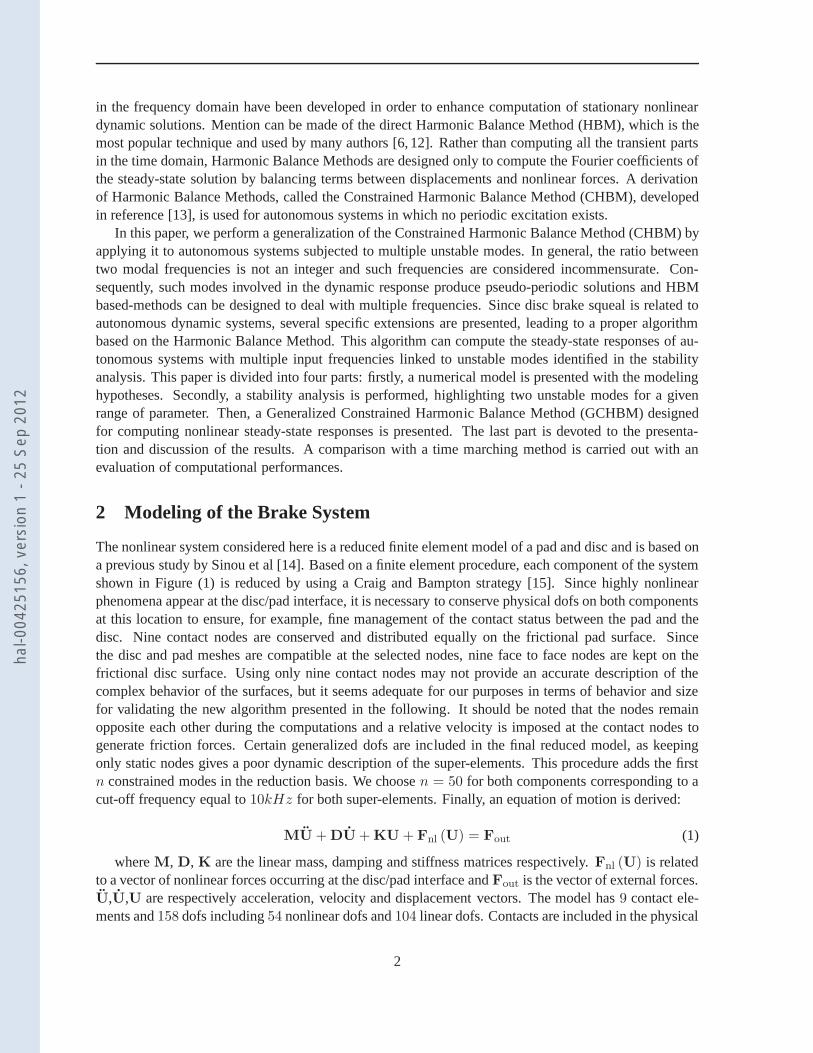
The nonlinear system considered here is a reduced finite element model of a pad and disc and is based ona previous study by Sinou et al [14]. Based on a finite element procedure, each component of the systemshown in Figure (1) is reduced by using a Craig and Bampton strategy [15]. Since highly nonlinearphenomena appear at the disc/pad interface, it is necessaryto conserve physical dofs on both componentsat this location to ensure, for example, fine management of the contact status between the pad and thedisc. Nine contact nodes are conserved and distributed equally on the frictional pad surface. Sincethe disc and pad meshes are compatible at the selected nodes,nine face to face nodes are kept on thefrictional disc surface. Using only nine contact nodes may not provide an accurate description of thecomplex behavior of the surfaces, but it seems adequate for our purposes in terms of behavior and sizefor validating the new algorithm presented in the following. It should be noted that the nodes remainopposite each other during the computations and a relative velocity is imposed at the contact nodes togenerate friction forces. Certain generalized dofs are included in the final reduced model, as keepingonly static nodes gives a poor dynamic description of the super-elements. This procedure adds the firstn constrained modes in the reduction basis. We choosen = 50 for both components corresponding to acut-off frequency equal to10kHz for both super-elements. Finally, an equation of motion is derived:
MU+DU+KU+ Fnl (U) = Fout (1)
whereM, D, K are the linear mass, damping and stiffness matrices respectively. Fnl (U) is relatedto a vector of nonlinear forces occurring at the disc/pad interface andFout is the vector of external forces.U,U,U are respectively acceleration, velocity and displacementvectors. The model has9 contact ele-ments and158 dofs including54 nonlinear dofs and104 linear dofs. Contacts are included in the physical
2
hal-0
0425
156,
ver
sion
1 -
25 S
ep 2
012
Figure 1: Split view of the finite element model of the brake system. The red dots represent the contactnodes
systems to add constraints in the equation of motion (1). Forconvenience, we choose to consider thepenalty method. Springs are added at the disc/pad interfaceto impose contact conditions. Measurementsof pad compressibility show a nonlinear relationship between the pressure and the displacement. This ef-fect is included at the interfaces where nonlinear contact stiffnesses are considered in our model. Finally,the mathematical function used to describe the contact force is:
Fcontact,i =
kl (u1 − u2) + knl(u1 − u2)3 if (u1 − u2) > 0
0 otherwise(2)
whereu1 andu2 are respectively displacements of contact nodes of the pad and disc at contact elementi. For the frictional definition, we consider a simplified Coulomb law with a constant friction coefficientwithout stick-slip motion. Moreover, a unidirectional friction effort is considered. Then a friction forceFf,i located at nodei is derived from a contact effortFcontact,i with:
Ff,i = µFcontact,isgn(vr,i) (3)
whereµ is the friction coefficient andvr,i the relative velocity between the disc and pad at nodei.The damping matrixD is built by considering a Rayleigh damping withα andβ chosen to obtain modaldampingζ = 0.1 on non-frictional coupled modes900Hz and940Hz. The external force is directlyapplied on the back pad on four nodes for almost piston like pressure distribution. Table 1 provides themodel parameters. To enhance understanding, it may be notedthat the chosen finite element model (withthe contact and damping assumption) does not attempt to capture all effects realistically. This modelinghas been chosen to illustrate a suitable range of behavior and to investigate the efficiency of the proposednon-linear method.
3 Static computation and stability analysis
The classical tool for predicting unstable modes in squeal analysis is a linear computation consisting infinding unstable modes around a linearized static position.The first step considers only the static part of
3
hal-0
0425
156,
ver
sion
1 -
25 S
ep 2
012
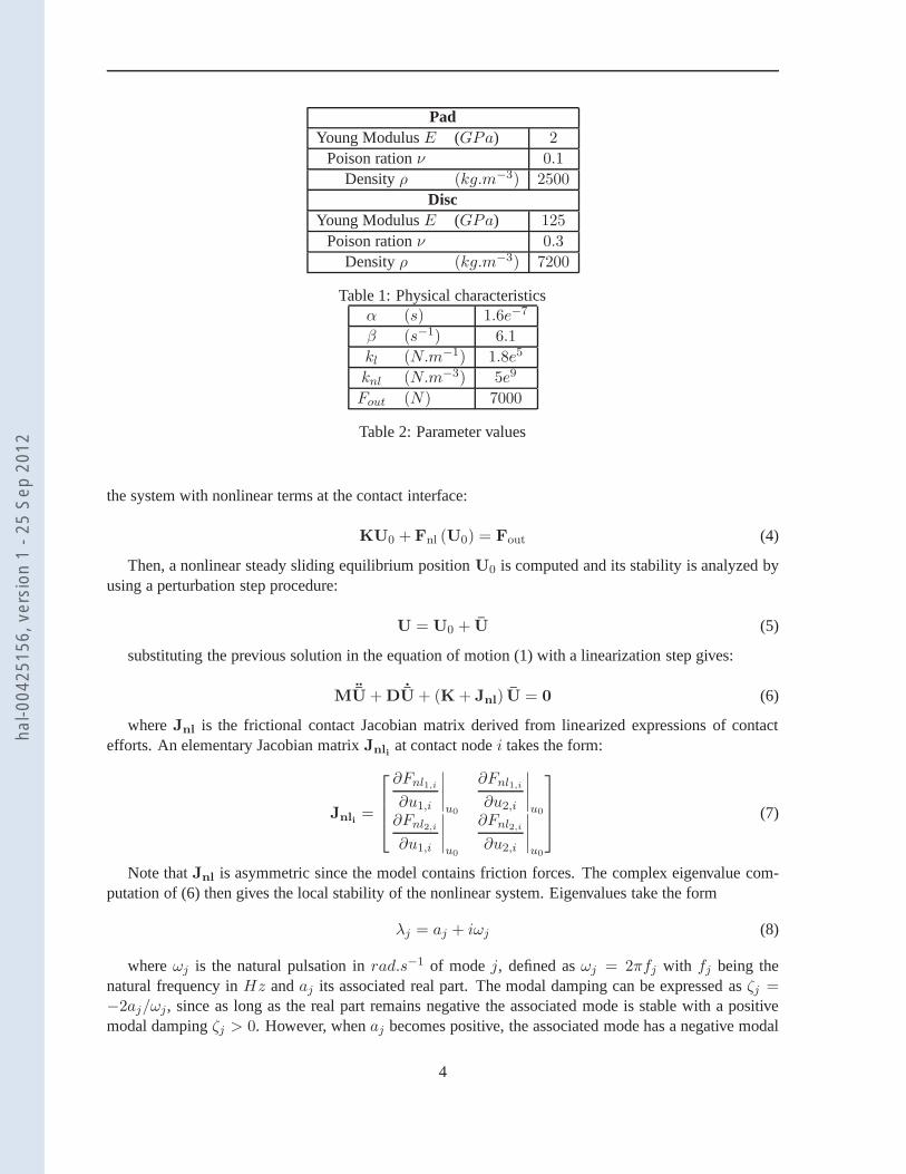
PadYoung ModulusE (GPa) 2
Poison rationν 0.1
Densityρ (kg.m−3) 2500
DiscYoung ModulusE (GPa) 125
Poison rationν 0.3
Densityρ (kg.m−3) 7200
Table 1: Physical characteristicsα (s) 1.6e−7
β (s−1) 6.1
kl (N.m−1) 1.8e5
knl (N.m−3) 5e9
Fout (N) 7000
Table 2: Parameter values
the system with nonlinear terms at the contact interface:
KU0 +Fnl (U0) = Fout (4)
Then, a nonlinear steady sliding equilibrium positionU0 is computed and its stability is analyzed byusing a perturbation step procedure:
U = U0 + U (5)
substituting the previous solution in the equation of motion (1) with a linearization step gives:
M¨U+D
˙U+ (K+ Jnl) U = 0 (6)
whereJnl is the frictional contact Jacobian matrix derived from linearized expressions of contactefforts. An elementary Jacobian matrixJnli at contact nodei takes the form:
Jnli =
∂Fnl1,i
∂u1,i
∣
∣
∣
∣
u0
∂Fnl1,i
∂u2,i
∣
∣
∣
∣
u0
∂Fnl2,i
∂u1,i
∣
∣
∣
∣
u0
∂Fnl2,i
∂u2,i
∣
∣
∣
∣
u0
(7)
Note thatJnl is asymmetric since the model contains friction forces. Thecomplex eigenvalue com-putation of (6) then gives the local stability of the nonlinear system. Eigenvalues take the form
λj = aj + iωj (8)
whereωj is the natural pulsation inrad.s−1 of modej, defined asωj = 2πfj with fj being thenatural frequency inHz andaj its associated real part. The modal damping can be expressedasζj =−2aj/ωj, since as long as the real part remains negative the associated mode is stable with a positivemodal dampingζj > 0. However, whenaj becomes positive, the associated mode has a negative modal
4
hal-0
0425
156,
ver
sion
1 -
25 S
ep 2
012
a b
0.1 0.15 0.2 0.25 0.3 0.35 0.4 0.45 0.5
900
920
940
Friction Coefficient
Fre
quen
cy (
Hz)
0.1 0.15 0.2 0.25 0.3 0.35 0.4 0.45 0.51505
1510
1515
Friction Coefficient
Fre
quen
cy (
Hz)
0.1 0.15 0.2 0.25 0.3 0.35 0.4 0.45 0.5
−200
0
200
Friction Coefficient
Rea
l Par
t
0.1 0.15 0.2 0.25 0.3 0.35 0.4 0.45 0.5
−40
−20
0
20
Friction Coefficient
Rea
l Par
t
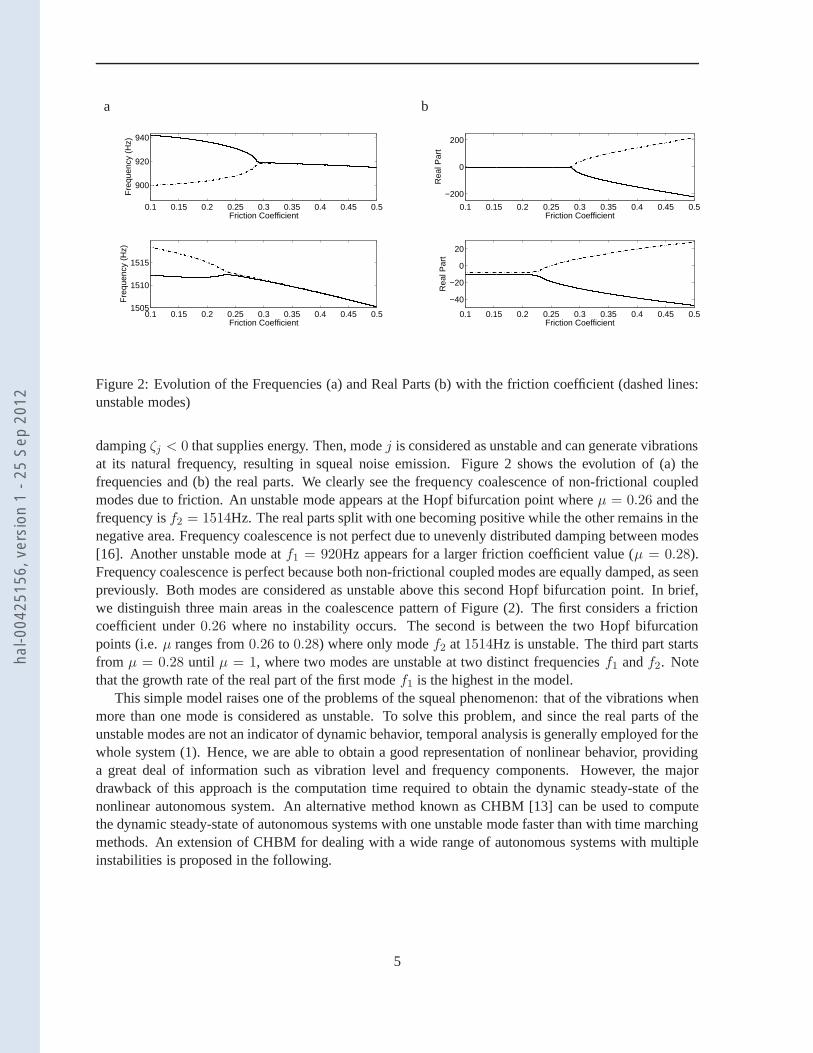
Figure 2: Evolution of the Frequencies (a) and Real Parts (b)with the friction coefficient (dashed lines:unstable modes)
dampingζj < 0 that supplies energy. Then, modej is considered as unstable and can generate vibrationsat its natural frequency, resulting in squeal noise emission. Figure 2 shows the evolution of (a) thefrequencies and (b) the real parts. We clearly see the frequency coalescence of non-frictional coupledmodes due to friction. An unstable mode appears at the Hopf bifurcation point whereµ = 0.26 and thefrequency isf2 = 1514Hz. The real parts split with one becoming positive while theother remains in thenegative area. Frequency coalescence is not perfect due to unevenly distributed damping between modes[16]. Another unstable mode atf1 = 920Hz appears for a larger friction coefficient value (µ = 0.28).Frequency coalescence is perfect because both non-frictional coupled modes are equally damped, as seenpreviously. Both modes are considered as unstable above this second Hopf bifurcation point. In brief,we distinguish three main areas in the coalescence pattern of Figure (2). The first considers a frictioncoefficient under0.26 where no instability occurs. The second is between the two Hopf bifurcationpoints (i.e.µ ranges from0.26 to 0.28) where only modef2 at 1514Hz is unstable. The third part startsfrom µ = 0.28 until µ = 1, where two modes are unstable at two distinct frequenciesf1 andf2. Notethat the growth rate of the real part of the first modef1 is the highest in the model.
This simple model raises one of the problems of the squeal phenomenon: that of the vibrations whenmore than one mode is considered as unstable. To solve this problem, and since the real parts of theunstable modes are not an indicator of dynamic behavior, temporal analysis is generally employed for thewhole system (1). Hence, we are able to obtain a good representation of nonlinear behavior, providinga great deal of information such as vibration level and frequency components. However, the majordrawback of this approach is the computation time required to obtain the dynamic steady-state of thenonlinear autonomous system. An alternative method known as CHBM [13] can be used to computethe dynamic steady-state of autonomous systems with one unstable mode faster than with time marchingmethods. An extension of CHBM for dealing with a wide range ofautonomous systems with multipleinstabilities is proposed in the following.
5
hal-0
0425
156,
ver
sion
1 -
25 S
ep 2
012
4 Generalized Harmonic Balance Method
4.1 Quasi periodic functions
Responses are no longer periodic when oscillatory systems are subjected top incommensurable fre-quencies. The nonlinear oscillations contain the frequency components of any linear combination of theincommensurable frequency components
k1ω1 + k2ω2 + · · ·+ kjωj + · · ·+ kpωp (9)
with ki = −Nh,−Nh + 1, . . . ,−1, 0, 1, . . . , Nh − 1, Nh for i = 1, . . . , p. Nh defines the order for eachfundamental frequency andp the number of incommensurable frequencies.
Thus the dynamic solution of equation (1) can be expressed with a generalized Fourier series suchthat:
U (t) ≈
Nh∑
k1=−Nh
. . .
Nh∑
kp=−Nh
ak1...kpcos (k1ω1 + . . .+ kpωp) t+ bk1...kp
sin (k1ω1 + . . .+ kpωp) t
(10)ak1,...,kp
andbk1,...,kpdefine the unknown Fourier coefficients of any linear combinations of the
incommensurable frequency componentsω1, ω2, . . . , ωp that have been defined previously in (9).The previous expression can be rewritten in a condensed form
U (t) = a0 +∑
k∈Zp
ak cos (k.ω) t+∑
k∈Zp
bk sin (k.ω) t (11)
where the(.) denotes the dot product,k is the harmonic number vector of each frequency direction andω is the vector of thep incommensurable frequencies considered in the solution. For convenience, it iswise to deal with a multiple time parameterτ such that
τ = ωt (12)
and equation (11) is rewritten as
U (τ ) = a0 +∑
k∈Zp
ak cos (k.τ ) +∑
k∈Zp
bk sin (k.τ ) (13)
whereτ = [τ1 . . . τp] is a non dimensional time parameter and refers to thehyper-time conceptproposed by [17]. Consequently, rather than dealing with a single time domaint ∈ R+ for solutionU(t), a multiple periodic time domainτ ∈ R
p+ is considered where each dimensionτj corresponds to
one incommensurable fundamental frequency identified in the solution. Therefore (13) is2π periodicon every hyper-time dimension ofτ . U(τ ) representsU(t) in a p dimensional time space where eachfrequency is independent from the others. For example, Schilder et al. [18] definetorus functions whichrepresent the hyper-time domain in a3 dimensional space for2 incommensurate frequencies. An analogywith numerical image processing can be considered to illustrate thehyper-time concept when applyinga filter on an image. It can be considered as a visual signal depending on both parameters, its twoorthogonal directions(x, y) that are similar toτ1 andτ2 in a hyper-time domain.
Theoretically, (13) is able to treat a great range of aperiodic dynamic systems where a finite numberof p incommensurable frequencies have been identified. A definition given by [17] for definingNh
harmonics in a multiple Fourier series is:
6
hal-0
0425
156,
ver
sion
1 -
25 S
ep 2
012
p∑
j=1
|kj | ≤ Nh (14)
This choice is justified by the fact that the major part of the signal energy is generally included in thevery first harmonics and the very first coupling frequencies.
Equation (14) will be used in the following for the multiple Fourier series truncation.
4.2 Generalized Harmonic Balance Method
Substituting (11) in the behavior equation (1) and considering equation (14) gives:
R (t) ≈∑
k∈ZnNh
[(
K− (k.ω)2 M)
ak + ((k.ω)D)bk
]
cos (k.τ )+
∑
k∈ZnNh
[(
K− (k.ω)2 M)
bk − ((k.ω)D)ak
]
sin (k.τ ) + Fnl (ak,bk)− Fout
(15)
Since sine and cosine are orthogonal functions, they are used as bases and we use a Galerkin procedurefor computing Fourier coefficients:
∫ 2π
0
. . .
∫ 2π
0
R cos (k1.τ1 + . . . + kp.τp) dτ1 . . . dτp = 0 for all kj suchp
∑
j=1
|kj | ≤ Nh
∫ 2π
0
. . .
∫ 2π
0
R sin (k1.τ1 + . . . + kp.τp) dτ1 . . . dτp = 0 for all kj suchp
∑
j=1
|kj | ≤ Nh
(16)
And the following set of algebraic equations is derived:
Λz+ Fnl (z) = Fout (17)
WhereΛ refers to the block diagonal dynamic stiffness matrix:
Λ =
K 0 0 0 0 0
0 Λ1 0 0 0 0
0 0. . . 0 0 0
0 0 0 Λi 0 0
0 0 0 0. . . 0
0 0 0 0 0 ΛNc
(18)
with
Λi =
[
− (k.ω)2 M+K (k.ω)D
− (k.ω)D − (k.ω)2M+K
]
for i ∈ [1, Nc] (19)
Nc represents the total number of frequency components including all harmonic terms up toNh ofeach frequency direction and all the coupling frequencies chosen by using (14). They must also be
7
hal-0
0425
156,
ver
sion
1 -
25 S
ep 2
012
positive. ThereforeNc depends onωk values. A particular case wherep = 2 is studied in the followingand thusNc is defined.
z, Fnl (z) and Fout are respectively the Fourier coefficient vectors of displacement, nonlinear fric-tional contact forces and external forces of the system. They are expressed as:
z =[
a0 a1 b1 · · · aNcbNc
]
(20)
Fnl =[
Fnl,0 Fanl,1 F
bnl,1 · · · F
anl,Nc
Fbnl,Nc
]
(21)
Fout =[
Fout,0 Faout,1 F
bout,1 · · · F
aout,Nc
Fbout,Nc
]
(22)
Since the behavior ofFnl is nonlinear with respect to the displacement vector, equation (17) must besolved iteratively by using Newton-Raphson root-finding algorithms. The analytical computation ofFnl
in the frequency domain is prohibitive when defined as a piecewise nonlinear function of displacement.To get round this issue, certain techniques have been developed for computing nonlinear terms. TheIncremental Harmonic Balance Method (IHBM) or High Dimensional Harmonic Balance Method (HD-HBM) [19,20] is applied to nonlinear systems under multipleexcitation frequencies. The nonlinear treat-ment of Fourier coefficients is performed by using multiple time scales where transformation matricesof equally spaced sub-time levels are built to compute the nonlinear Fourier coefficients. Cameron [21]proposes the Alternating-Frequency Time (AFT) method to compute the periodic nonlinear forces in thetime domain and then extract their exact Fourier coefficients Fnl. As we use ahyper-time domain wherethe functions are2π periodic on every orthogonal time dimension, the generalization of the AFT canbe extended to ap-dimensional frequency domain by using ap-dimensional FFT. The procedure is asfollows:
zIFFTp
−→ U (τ ) −→ Fnl (U(τ ))FFTp
−→ Fnl (z) (23)
OnceFnl (U(τ )) is evaluated, its Fourier coefficients are computed and injected into equation (17). Inbrief, GHBM is written as an objective functionJ1 of a dynamic system subjected to multiple frequencyinputs:
J1 (z) =∥
∥
∥Λz+ Fnl (z)− Fout
∥
∥
∥< ǫ1 (24)
where||.|| defines the euclidean norm andǫ1 is a chosen tolerance.
4.3 Additional constraint equations
This derivation of GHBM can be applied to a wide variety of dynamic systems exhibiting pseudo-periodic responses due to a finite number of identified exciting frequencies. As seen previously, discbrake squeal is equivalent to an autonomous system, i.e. thedynamic response implicitly depends ontime or, in other words, no external excitation forces excite the structure. Thus GHBM gives the trivialsolution in which the Fourier coefficients would be null except for the static components, even thougha local minimum exists for the dynamic steady-state in the optimization domain [13]. The existence ofboth solutions is related to the nature of the dynamic systemillustrated by equation (1). Under unstablestatic conditions, the system may or may not oscillate, depending only on the initial conditions or a per-turbation of the system’s parameters. Hence a set of additional equations has to be included in equation(17) to reach the minimum related to the dynamic solution.
8
hal-0
0425
156,
ver
sion
1 -
25 S
ep 2
012
If we consider that the nonlinear response of an autonomous system is driven byp unstable modes:
U(t) =
p∑
j=1
Ψjeϕjt (25)
whereΨj is an unstable mode andϕj = aj + iωj its eigenvalue. It can be seen thatΨj andϕj
depend implicitly onU(t) since they are subjected to nonlinear effects thus a change in contact status.Hence,[Ψ1 . . .Ψp]
T should be considered as unstable modes of a dynamic state with their correspondingcomplex eigenvalues[ϕ1 . . . ϕp]
T, as opposed to unstable modes of the sliding steady-state solution seenin section 3. Hence, when looking at equation (25), a null real part of ϕj indicates that the dynamicresponseUj(t) = Ψje
iωjt is stationary through time and oscillates with pulsationωj. Therefore, whenall p unstable modes have a null real part,Uj(t) becomes a pseudo-periodic motion that is the steady-state response of the autonomous system considered. Therefore minimizing the real parts of eigenvaluesϕj (with j ∈ [1, p]) in the optimization process would lead to the correct computation of the Fouriercoefficients linked to the steady-state solution.
The computation ofϕj is performed by considering an equivalent linear system to equation (1) andrefers to the equivalent linear concept proposed by Iwan [22, 23] where the nonlinear termsFnl (U(t))are replaced with a linear approximation matrixJnl such that:
ζ = Fnl (U(t)) − JnlU(t) with ζ → 0 (26)
Jnl refers to a time independent Jacobian matrix of the nonlinear temporal forcesFnl (U(t)) at thedynamic stationary stateU(t).
Since a Fourier Transformation is a linear application,Jnl can also be computed in the frequencydomain with Fourier coefficients:
ζ = Fnl (z)− Jnlz with ζ → 0 (27)
A good linear approximation of (1) is obtained whenζ → 0. Then (1) is substituted by:
MU+DU+ (K+ Jnl)U = Fout (28)
By using a perturbation method, the complex eigenvaluesϕ of equation (28) are computed and thepreal parts linked to the unstable modes are extracted and gathered in a vector, forming a second objectivefunctionJ2.
Secondly, since there is no external excitation, thep nonlinear pulsationsωj are undefined and thushave to be considered asp independent unknowns. In brief, a Generalized ConstrainedHarmonic Bal-ance Method (GCHBM) applicable to autonomous systems subjected top incommensurate frequencycomponents is arranged in a set of two objective functions:
J1 (z,Ω) =∥
∥
∥Λ (z,Ω) z+ Fnl (z,Ω)− Fout
∥
∥
∥< ǫ1
J2 (z,Ω) = ‖Re (ϕj (z,Ω))‖ < ǫ2 with j ∈ [1, p](29)
In more detailJ2 takes the form
J2 (z,Ω) =
‖Re (ϕ1 (z,Ω))‖‖Re (ϕ2 (z,Ω))‖
...‖Re (ϕp (z,Ω))‖
(30)
9
hal-0
0425
156,
ver
sion
1 -
25 S
ep 2
012
with vectorΩ of p unknown frequencies:
Ω =
ω1
ω2
...ωp
(31)
Computation is performed when< J1, J2 > are respectively below chosen tolerances< ǫ1, ǫ2 >.Such a set of objective functions has(n (1 + 2Nc) + p) equations to be solved with(n (1 + 2Nc) + p)unknowns and is therefore well-determined.n is the dimension of the dynamic system,Nc is the totalnumber of frequency combinations andp is the number of unstable modes used in the solution.
4.4 Reduction step
The computation time of any nonlinear system is related to the number of unknowns so any reduction inthe size of the system would increase performance. The authors of [24] propose a reduction method fornonlinear systems studied in the frequency domain without loss of accuracy. After reorganizing linearand nonlinear dofsznl andzln, the system described by equation (17) can be expressed as follows:
[
Λln,ln Λln,nl
Λnl,ln Λnl,nl
]
zln
znl
+
0
Fnl
=
Fout,ln
Fout,nl
(32)
and equation (17) is rewritten in term of nonlinear components such that:
Λeqznl + Fnl (znl) = Feq (33)
withΛeq = Λnl,nl −Λnl,ln (Λln,ln)
−1Λln,nl (34)
andFeq = Fout,nl −Λnl,ln (Λln,ln)
−1Fout,ln (35)
This step reduces the number of equations from(n (2Nc + 1) + p) to (nnl (2Nc + 1) + p) wherenandnnl are the numbers of total dofs and nonlinear dofs respectively. Thus this reduction step is veryefficient for large systems with only few nonlinear dofs. When znl is known,zln is easily obtained by:
zln = Λ−1ln,ln
(
Fout,ln −Λln,nlznl
)
(36)
Hence, a reduced form of equation (29) is:
J1 (znl,Ω) =∥
∥
∥Λeq (znl,Ω) znl + Fnl (znl,Ω)− Feq
∥
∥
∥< ǫ1
J2 (znl,Ω) = ‖Re (ϕj (znl,Ω))‖ < ǫ2 with j ∈ [1, p](37)
Computation is done when< J1, J2 > are respectively below chosen tolerances< ǫ1, ǫ2 >. Figure3 represents the general algorithm procedure of a GCHBM.
10
hal-0
0425
156,
ver
sion
1 -
25 S
ep 2
012
4.5 GCHBM initialization
Regarding time marching methods, optimization processes need a starting point to find a solution inthe optimization domain. A bad choice of initial conditionsis synonymous with slow convergence.As explained in [13] and inspired by the concept of Complex Non Linear Modal Analysis (CNLMA)developed by Sinou et al. [25], Fourier coefficients of the first harmonic are initialized by the unstablemode vectors found in the stability analysis. This is based on the assumption that dynamic behavioris mainly driven by unstable modes. Thus for every first harmonic (in Fourier basis) of every unstablemode, the initial prediction takes the form:
z1,j = η(
Ψj + Ψj
)
with j ∈ [1, p] (38)
whereΨj defines thejth nonlinear unstable mode shape,Ψj is its conjugate andη is an arbitrarilychosen coefficient with a range from20 to 60 to ensure convergence of the optimization problem. As canbe observed, the pulsations area priori unknown while a good initial estimate considers those foundinthe stability analysis.
5 Application to squeal vibration
5.1 Brake model with two unstable modes
As indicated previously in section 3, two modes are found to be unstable, with the potential to vibrate.Thus,J2 andΩ are two-dimensional and take the following form:
J2 (znl,Ω1−2) =
‖Re (ϕ1 (znl,Ω1−2))‖‖Re (ϕ2 (znl,Ω1−2))‖
(39)
Ω1−2 =
ω1
ω2
(40)
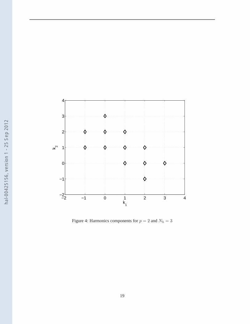
A geometric interpretation ofk ∈ Z2 (i.e. p = 2 andNh = 3) is given in Figure 4. It can be seen
that the harmonic combinations are constrained by equation(14) and that the resulting frequencies arepositive.
According to Figure 4,Nc = 12 and as seen in section 2, the nonlinear terms are equal tonnl = 54.Thus the whole equation set has1352 unknowns and equations. It should be noted that for the case wherek1 = k2 = 0 stands for the static Fourier coefficients and is not included inNc.
5.2 Nonlinear Steady-State
In this section, the results of the GCHBM procedure and comparisons with temporal results from refer-ence [14] are presented and discussed. Steady-state solutions for three different friction coefficients arestudied. The efficiency of GCHBM is underlined as are the optimization process parameters. Finally,results relating to the evolution of frequencies and amplitude level as a function of friction coefficient arediscussed. Table 2 groups the parameter values and Table 3 gathers frequency values for three differentfriction coefficients.
11
hal-0
0425
156,
ver
sion
1 -
25 S
ep 2
012
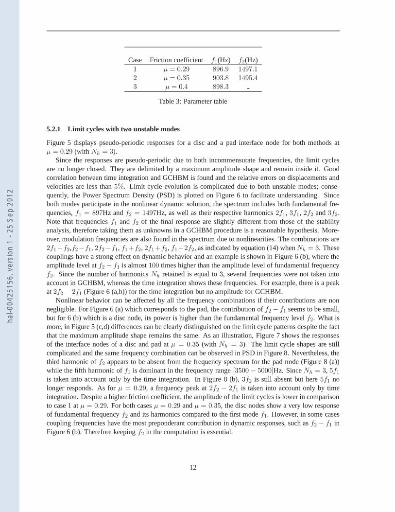
Case Friction coefficient f1(Hz) f2(Hz)1 µ = 0.29 896.9 1497.12 µ = 0.35 903.8 1495.43 µ = 0.4 898.3
Table 3: Parameter table
5.2.1 Limit cycles with two unstable modes
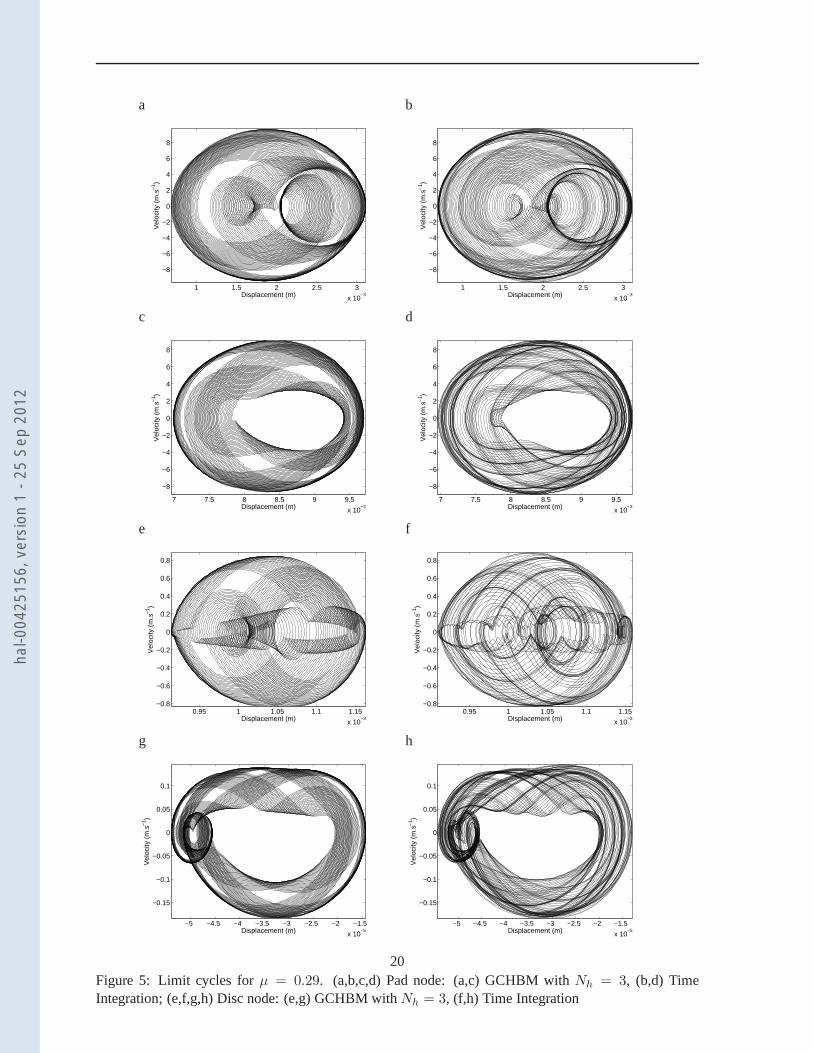
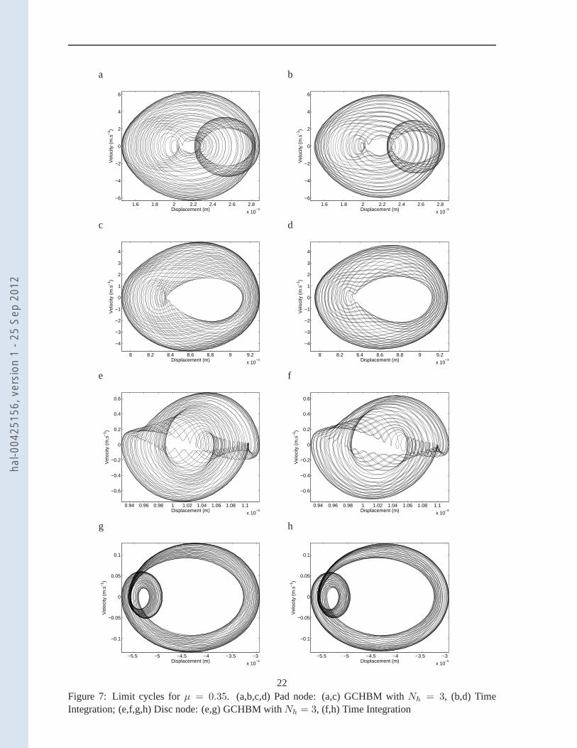
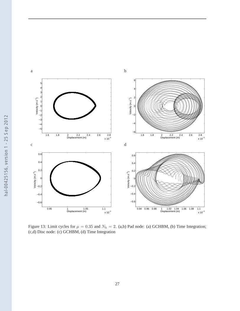
Figure 5 displays pseudo-periodic responses for a disc and apad interface node for both methods atµ = 0.29 (with Nh = 3).
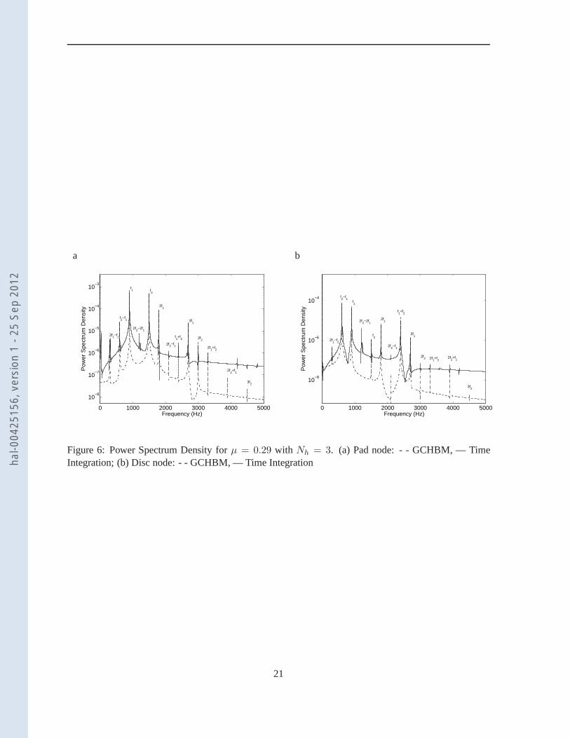
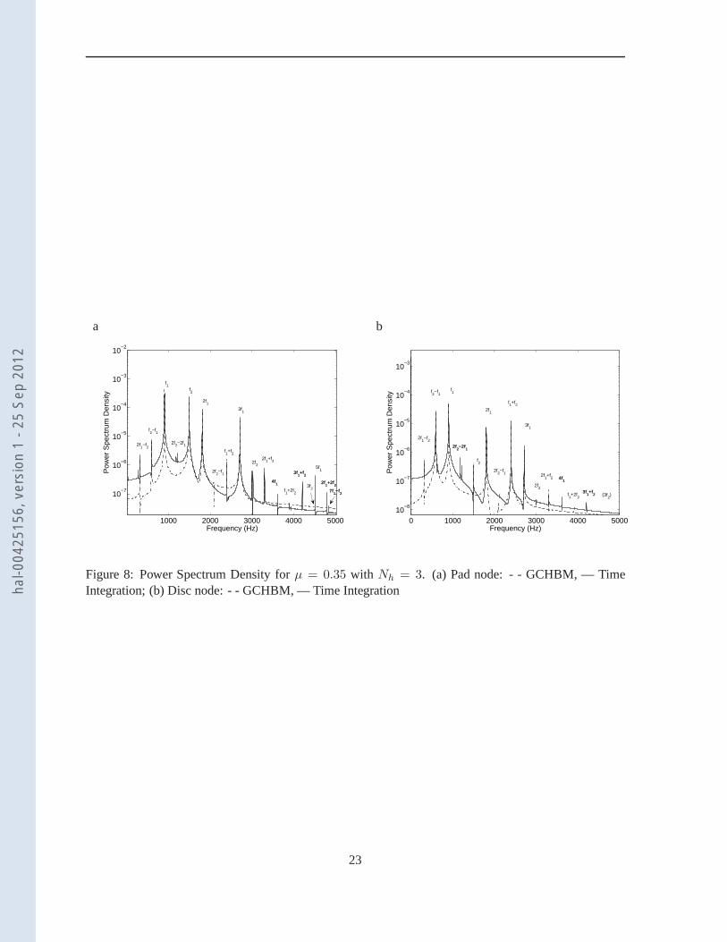
Since the responses are pseudo-periodic due to both incommensurate frequencies, the limit cyclesare no longer closed. They are delimited by a maximum amplitude shape and remain inside it. Goodcorrelation between time integration and GCHBM is found andthe relative errors on displacements andvelocities are less than5%. Limit cycle evolution is complicated due to both unstable modes; conse-quently, the Power Spectrum Density (PSD) is plotted on Figure 6 to facilitate understanding. Sinceboth modes participate in the nonlinear dynamic solution, the spectrum includes both fundamental fre-quencies,f1 = 897Hz andf2 = 1497Hz, as well as their respective harmonics2f1, 3f1, 2f2 and3f2.Note that frequenciesf1 andf2 of the final response are slightly different from those of thestabilityanalysis, therefore taking them as unknowns in a GCHBM procedure is a reasonable hypothesis. More-over, modulation frequencies are also found in the spectrumdue to nonlinearities. The combinations are2f1−f2,f2−f1, 2f2−f1, f1+f2, 2f1+f2, f1+2f2, as indicated by equation (14) whenNh = 3. Thesecouplings have a strong effect on dynamic behavior and an example is shown in Figure 6 (b), where theamplitude level atf2 − f1 is almost100 times higher than the amplitude level of fundamental frequencyf2. Since the number of harmonicsNh retained is equal to3, several frequencies were not taken intoaccount in GCHBM, whereas the time integration shows these frequencies. For example, there is a peakat2f2 − 2f1 (Figure 6 (a,b)) for the time integration but no amplitude for GCHBM.
Nonlinear behavior can be affected by all the frequency combinations if their contributions are nonnegligible. For Figure 6 (a) which corresponds to the pad, the contribution off2 − f1 seems to be small,but for 6 (b) which is a disc node, its power is higher than the fundamental frequency levelf2. What ismore, in Figure 5 (c,d) differences can be clearly distinguished on the limit cycle patterns despite the factthat the maximum amplitude shape remains the same. As an illustration, Figure 7 shows the responsesof the interface nodes of a disc and pad atµ = 0.35 (with Nh = 3). The limit cycle shapes are stillcomplicated and the same frequency combination can be observed in PSD in Figure 8. Nevertheless, thethird harmonic off2 appears to be absent from the frequency spectrum for the pad node (Figure 8 (a))while the fifth harmonic off1 is dominant in the frequency range[3500 − 5000]Hz. SinceNh = 3, 5f1is taken into account only by the time integration. In Figure8 (b), 3f2 is still absent but here5f1 nolonger responds. As forµ = 0.29, a frequency peak at2f2 − 2f1 is taken into account only by timeintegration. Despite a higher friction coefficient, the amplitude of the limit cycles is lower in comparisonto case1 atµ = 0.29. For both casesµ = 0.29 andµ = 0.35, the disc nodes show a very low responseof fundamental frequencyf2 and its harmonics compared to the first modef1. However, in some casescoupling frequencies have the most preponderant contribution in dynamic responses, such asf2 − f1 inFigure 6 (b). Therefore keepingf2 in the computation is essential.
12
hal-0
0425
156,
ver
sion
1 -
25 S
ep 2
012
5.2.2 Choice and influence of the harmonic number
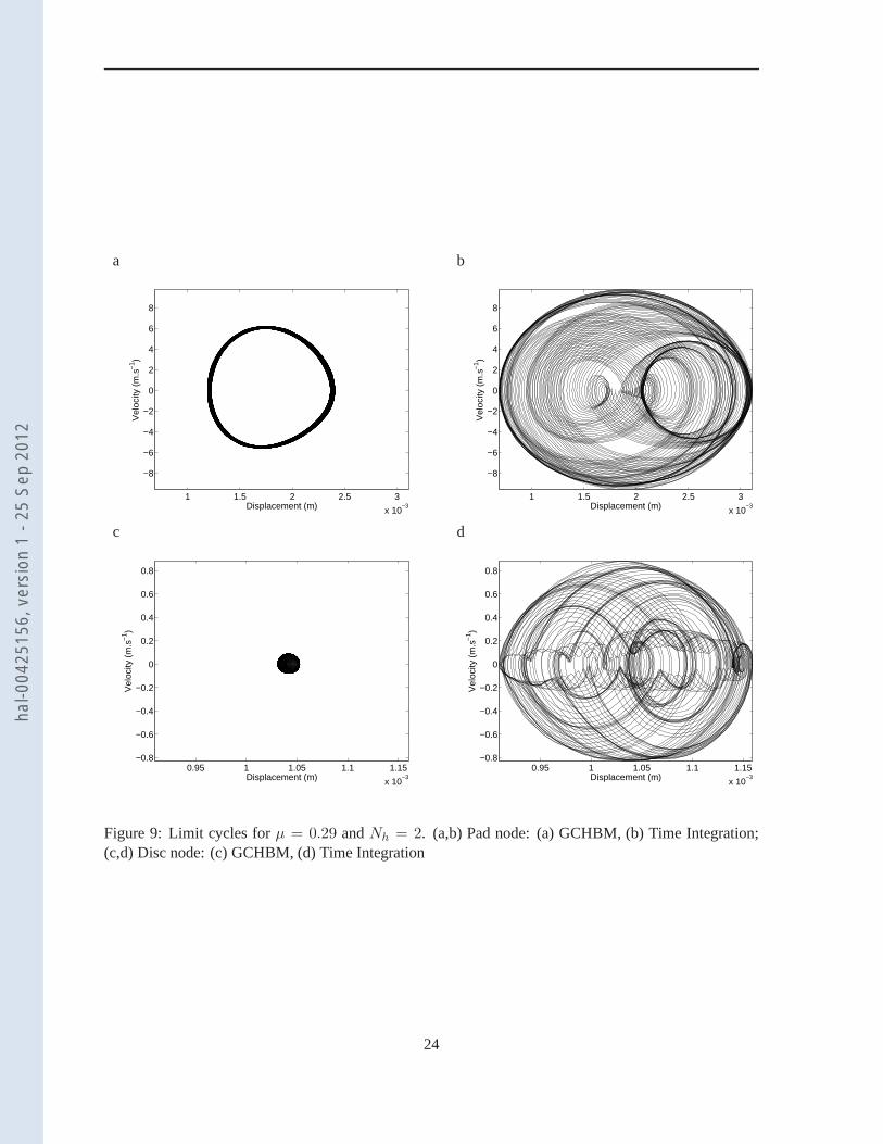
A common problem when dealing with harmonic balance methodsis making the right choice of har-monic numbers to compute a solution. An excessively low number could lead to a poor estimation of theresponse, especially if strong nonlinearities exist, but choosing too many harmonics leads to unnecessar-ily intensive computation. Consequently, a compromise must be found. By way of example, we try tocompute a nonlinear solution with the following parameters, (Nh = 2, µ = 0.29) under the same initialconditions as for(Nh = 3, µ = 0.29). It should be recalled that these initial conditions are derived fromsection 4.5.
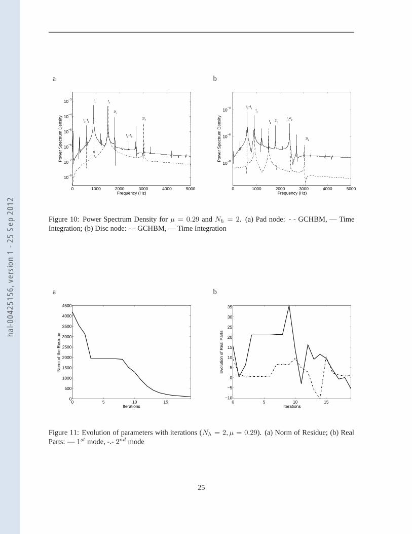
In Figure 9, the GCHBM withNh = 2 are wrong, compared to those of the time integration, asseen in Figure 10 where the harmonic components of GCHBM do not fit with those from the temporalintegration. When looking at the convergence chart in Figure 11, it can be seen thatǫ1 has not reacheda minimum (Figure 11 a) and the real partsa1 anda2 that describeǫ2 (Figure 11 b) are not minimizedsincea1 ≈ −6.1 anda2 ≈ 2. The solver stopped because it could not find any downward direction.
One of the reasons for this could be the fact that the restricted number of harmonics leads to an over-large approximation of displacements and thus of the nonlinear forces used for the dynamic Jacobiancomputation, see equation (27). Therefore the criterionǫ2 derived from the real parts associated with thecomplex eigenvalues applied for equation (30) would not be satisfied.
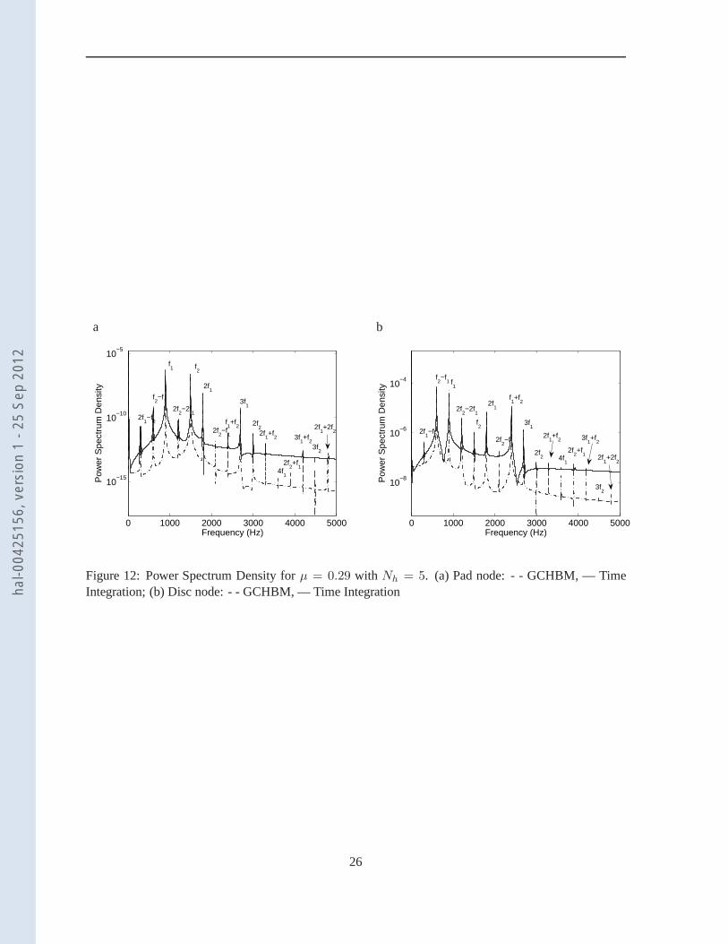
Regarding validation, Figure 12 displays the density of thepower spectra when usingNh = 5 forµ = 0.29. As expected, higher harmonics such as4f1, 5f1, 4f2, 5f2, 2f2 − 2f1, 3f1 − f2 and2f1 +2f2are found in the spectrum and the GCHBM pattern is very similar to the temporal pattern. However, theamplitude of these high frequency harmonics is negligible when compared to those found withNh = 3and they do not appear to affect the stationary response.
Now we considerNh = 2 in a sequential continuation where we re-use the previous results as initialconditions for a solution computed with a new set of parameters. In practice, the computation is per-formed from< Nh = 3, µ = 0.345 > to < Nh = 2, µ = 0.35 >. The advantage of this procedure isthat we can determine whether, under better initial conditions, GCHBM is able to provide good resultswith fewer harmonics. The response is no, as indicated by figure 13, where the limit cycles computedby GCHBM are still far from the temporal solution. In Figure 14 it can be seen that the harmonic com-ponentsf1 and2f1 merge with those of the temporal integration, butf2, 2f2 are almost absent fromthe spectrum. Combination frequencies such asf2 − f1 or f2 + f1 are also badly computed, meaningthat usingNh = 2 in such cases is unsatisfactory. ThereforeNh = 3 seems to be a good compromisebetween accuracy and computation time and could be used in the following.
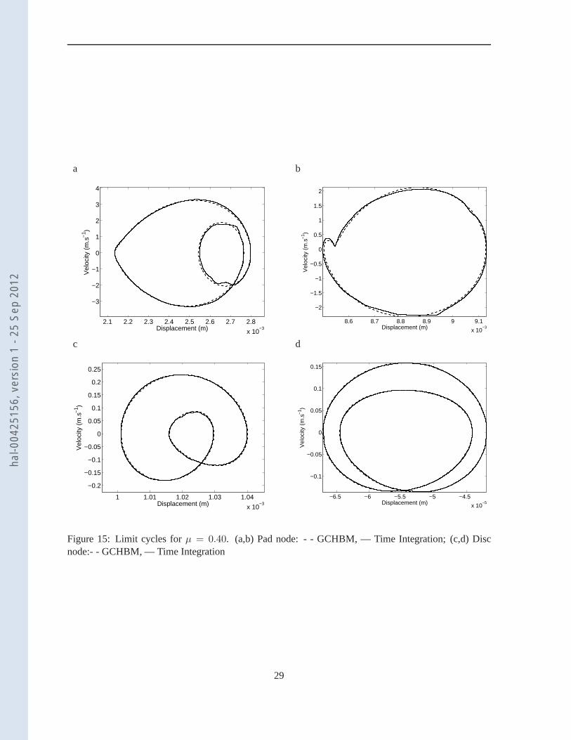
5.2.3 Limit cycles with one unstable mode
An interesting phenomenon appears when computing limit cycles for µ = 0.4. Figure 15 shows theresults of time integration and GCHBM procedure. To enhanceunderstanding, Figure 15(a) and (b) arefor two distinct pad nodes and Figure 15(c) and (d) are for twodistinct disc nodes.
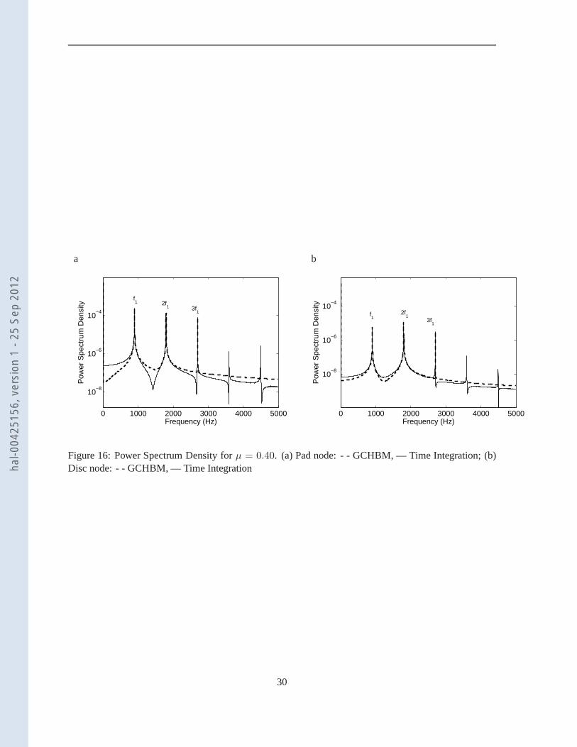
Although the stability analysis shows the presence of two unstable modes for this set of parameters,the dynamic behavior of the system is only driven by the first unstable modef1 = 898.3Hz and thesecond unstable modef2 is totally absent in the spectrum of Figure 16. Therefore only the fundamentalfrequencyf1 and its harmonics2f1 and3f1 are found and coupling frequencies such asf1 + f2, f2 −f1 and so on are no longer available. The inner loops in Figure 15(a) are due to the harmonics2f1and 3f1 exacerbated by nonlinearities. Obviously, sinceNh = 3 was chosen for the Fourier series,harmonics higher than3f1 are not computed and they are found to be absent from the GCHBMspectrum.
13
hal-0
0425
156,
ver
sion
1 -
25 S
ep 2
012
Nevertheless, these harmonics are not preponderant in the solution when comparing their power densityto the three first harmonics.
As seen previously, the GCHBM results are close to the time integration results with a relative erroron displacement less than1%. Note that GCHBM functions like a CHBM when only one unstablemodeis considered in the final solution.
5.3 Parameter evolution according toµ
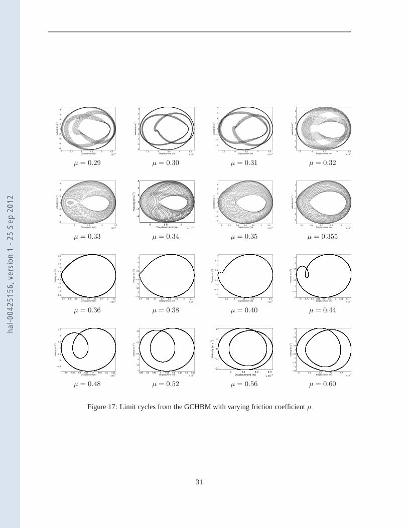
In this section we present the evolution of limit cycles withassociated unstable frequencies and the totalamplitude energy of the system withµ varying fromµ = 0.29 up toµ = 0.60 which is a part of theunstable domain. Figure 17 shows a set of limit cycles computed at different friction coefficient values.As seen previously, both modes are involved in the dynamic for a low friction coefficient with a complexlimit cycle shape. Whenµ is above0.36, we found closed limit cycles, indicating that only one moderemains in the dynamic.
To study the squeal propensity of each mode, an index was defined and the following were chosenfrom the literature:
αj = 100 ∗ 2Re(λj)
Im(λj)for thejth mode (41)
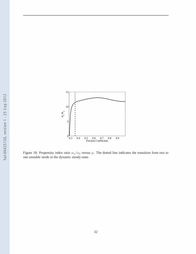
The ratioα1/α2 versus the friction coefficientµ is displayed in Figure 18. It is interesting to comparehow the ratio behaves withµ and its effects on the dynamic steady-state. When looking atthe first partof the curve, i.e. for0.29 < µ < 0.36, a very steep slope can be seen, but fromµ = 0.36 ratio α1/α2
remains almost constant with respect toµ. When looking at Figure 17 it can be seen that the transitionbetween a pseudo-periodic response to a periodic response also occurs at aroundµ = 0.36. It seems asif there is an analogy between the transition of the index ratios of both modes and their availability ornon-availability in the dynamic response. The ratio increases until the first modem1 replaces the secondmodem2 and remains constant whenm1 is the only mode providing a response.
As can be seen, a squeal propensity index higher by tenfold isfound for the1st mode compared tothe2nd mode atµ = 0.4. The energy of the first mode appears to replace the second mode even if thelatter is present in the stability analysis.
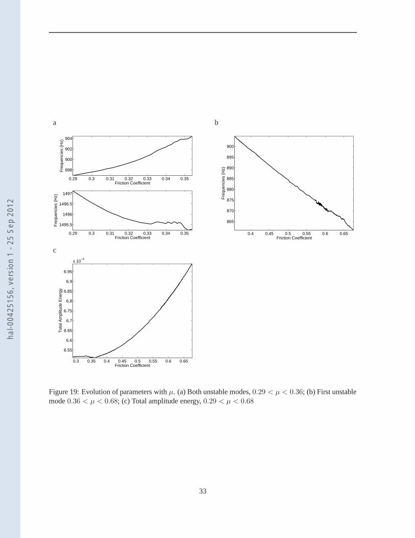
To facilitate understanding, Figure 19 (a) shows frequencies forµ varying fromµ = 0.29 to µ =0.36 where both modes are unstable. The frequencies are frictioncoefficient dependent, and whilef2decreases asµ increases, the slope off1 curve is positive in this range. Nevertheless,f2 disappears fromthe dynamic steady-state at aroundµ = 0.36 as can be seen in Figure 19 (b) where only the first unstablemodef1 is present in the limit cycle in the range betweenµ = 0.36 to µ = 0.68. Frequencyf1 followsa negative slope regardingµ, it decreases from905Hz atµ = 0.36 to 860Hz atµ = 0.68.
Figure 19 (c) shows the total amplitude energy of the whole system forµ ranging from0.29 to 0.68.In the first part, untilµ = 0.36 where both modes are unstable, the energy decreases and a minimumis found whenf2 vanishes from the solution. Fromµ = 0.36, the energy of the system increases witha quadratic form with respect toµ. The first unstable modef1 seems to act as energy pulsating in theactive range of the second modef2 before it disappears from the solution. As described above,thefriction coefficient not only modifies the amplitude of the dynamic behavior of autonomous systems,but it also influences their frequencies. This dependency between friction and frequency could have aneffect on neighboring modes by exciting them. Consequently, they may participate in the final dynamicsolution.
14
hal-0
0425
156,
ver
sion
1 -
25 S
ep 2
012
5.4 Convergence and Computation Time
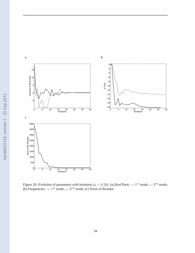
Convergence problems stem from many sources when attempting optimization. The main problems comefrom initial estimates made far from the target solution. Here convergence is achieved with the GCHBMalgorithm because a set of conditions considered as optimized is used. For each iteration, Figure 20displays the norm of the real parts (a), both optimized frequencies (b), and the norm of the residue (c).More precisely, frequency plot (b) corresponds to the difference between the optimized frequencies andthose obtained by a stability analysis.
The total number of iterations isNiter = 35. The real parts both tend to zero at the end of theoptimization process, as does the norm of the residue. A net difference between the initial frequenciesobtained by the stability analysis and those at the end of optimization is shown. For the first modef1, thefrequency evolution is about20Hz. GCHBM enhances computation time, which falls to about3 hours,20 minutes, whereas time integration needs about10 hours to obtain the dynamic steady-state. A betterconvergence result could be obtained by trying a new initialstarting point or by changing the tolerancevaluesǫ1 andǫ2, since Figure 20 clearly shows that both real parts and frequencies as well as the normof the residue have almost converged at iteration25. This would significantly reduce total computationtime. Here we have chosenǫ1 = ǫ2 = 0.01. It should be noted that these convergence results stem fromthe very first computation. When using another set of parameters, such as a change of friction coefficient,the results computed previously are injected as an initial starting point and computation is performed.Hence the number of iterations and thus computation time areconsiderably reduced, since only a fewiterations are required to converge to the final solution. Ingeneral, a new steady-state solution can becomputed in less than20 minutes.
6 Conclusion
In this paper we develop a new method called GCHBM able to compute the dynamic steady-states ofautonomous systems such as disc brake squeal in the case where stability analysis reveals large numbersof unstable modes. The computed solutions are either pseudo-periodic if at least two unstable modesgenerate vibrations, or periodic if dynamic behavior is driven by only one unstable mode. When at leasttwo unstable modes vibrate, the stationary dynamic responses become pseudo-periodic and the cycleplotted in the displacement-velocity coordinates is no longer closed. Particular care regarding the totalharmonic number must be considered to avoid missing important coupling frequencies or even the nonconvergence of the solver. Finally, GCHBM is well suited forbrake squeal analysis when a large numberof unstable modes are taken into account. It could help brakedesigners by computing the amplitudes oflimit cycles for sets of parameters faster than with time integration. Frequency responses are analyzedand modal behavior is better understood. For example, it detects the absence of the second modef2at µ = 0.36 although the stability analysis predicts two unstable modes. Dynamic behavior can becomputed for numerous parameter sets and an optimal area canbe found easily. For example, the lowestdynamic response of our model occurs atµ = 0.36 in the unstable area, the point at which the secondmodef2 disappears from the dynamic response.
Acknowledgements
Jean-Jacques Sinou gratefully acknowledges the financial support of the French National Research Agencythrough the Young Researcher program ANR-07-JCJC-0059-01-CSD 2.
15
hal-0
0425
156,
ver
sion
1 -
25 S
ep 2
012
References
[1] Kinkaid, N., O’Reilly, O., and Papadopoulos, P., 2003. “Automotive disc brake squeal”.Journal ofSound and Vibration, 267, pp. 105–166.
[2] Ouyang, H., Nack, W., Yuan, Y., and Chen, F., 2005. “Numerical analysis of automotive disc brakesqueal : a review”.International Journal of Vehicle Noise and Vibration, 1(3/4), pp. 207–231.
[3] Sinclair, D., and Manville, N.-J., 1955. “Frictional vibration”. Journal of Applied Mechanics,pp. 207–213.
[4] Spurr, R.-T., 1961-1962. “A theory of brake squeal”.Proceedings of the Institution of MechanicalEngineers, 1, pp. 33–40.
[5] Hoffmann, N., Fisher, M., Allgaier, R., and Gaul, L., 2002. “A minimal model for studying prop-erties of the mode-coupling type instability in friction induced oscillations”.Mechanics ResearchCommunications, 29, pp. 197–205.
[6] Sinou, J.-J., Thouverez, F., and Jezequel, L., 2004. “Methods to reduce non-linear mechanicalsystems for instability computation”.Archives of Computational Methods in Engineering - State ofthe art reviews, 11(3), pp. 257–344.
[7] Moirot, F., 1998. “Etude de la stabilite d’un equilibre en presence de frottement de coulomb,application au crissement des freins a disque”. PhD thesis, Ecole Polytechnique.
[8] Ouyang, H., Mottershead, J., Brookfield, D., James, S., and Cartmell, M., 2000. “Methodologyfor the determination of dynamic instabilities in a car discbrake”. International Journal of VehicleDesign, 23(3), pp. 241–262.
[9] Massi, F., Baillet, L., Giannini, O., and Sestieri, A., 2007. “Linear and non-linear numerical ap-proaches”.Mechanical Systems and Signal Processing, 21, pp. 2374–2393.
[10] AbuBakar, A., and Ouyang, H., 2006. “Complex eigenvalue analysis and dynamic transient anal-ysis in predicting disc brake squeal”.International Journal of Vehicle Noise and Vibration, 2(2),pp. 143–155.
[11] Lorang, X., Foy-Margiocchi, F., Nguyen, Q., and Gautier, P., 2006. “Tgv disc brake squeal”.Journal of Sound and Vibration, 293, pp. 735–746.
[12] Groll, G.-V., and Ewins, D.-J., 2001. “The harmonic balance method with arclength continuationin rotor/stator contact problems”.Journal of Sound and Vibration, 241(2), pp. 223–233.
[13] Coudeyras, N., Sinou, J.-J., and Nacivet, S., 2008. “A new treatment for predicting the self-excitedvibrations of nonlinear systems with frictional interfaces : The chbm”. Journal of Sound andVibration, 319, pp. 1175—1199.
[14] Sinou, J.-J., Coudeyras, N., and Nacivet, S., 2008. “Study of the nonlinear stationary dynamicof single and multi instabilities for disc brake squeal”.International Journal of Vehicle Design,51(1-2), pp. 207–222.
[15] Craig, R.-J., and Bampton, M., 1968. “Coupling of substructures for dynamic analyses”.AmericanInstitute of Aeronautics and Astronautics - Journal, 6(7), pp. 1313–1319.
16
hal-0
0425
156,
ver
sion
1 -
25 S
ep 2
012
[16] Fritz, G., Sinou, J.-J., Duffal, J.-M., and Jezequel, L., 2007. “Effects of damping on brake squealcoalescence patterns-application on a finite element model”. Mechanics Research Communications,34, pp. 181–190.
[17] Kim, Y.-B., and Choi, S.-K., 1997. “A multiple harmonicbalance method for the internal resonantvibration of a non-linear jeffcot rotor”.Journal of Sound and Vibration, 208(3), pp. 745–761.
[18] Schilder, F., Vogt, W., Schreiber, S., and Osinga, H.-M., 2005. Fourier methods for quasi-periodicoscillations. Tech. rep., Bristol Centre for Applied Nonlinear Mathematics.
[19] Chua, L.-O., and Ushida, A., 1981. “Algorithm for computing almost periodic steady-state responseof nonlinear systems to multiple input frequencies”.IEEE Transactions on Circuits and Systems,28(10), pp. 953–971.
[20] Ushida, A., and Chua, L.-O., 1984. “Frequency-domain analysis of nonlinear circuits driven bymulti-tone signals”.IEEE Transactions on Circuits and Systems, 31(9), pp. 766–778.
[21] Cameron, T. M., and Griffin, J. H., 1989. “An alternatingfrequency/time domain method for cal-culating the steady-state response of nonlinear dynamic systems”. Journal of Applied Mechanics,56(1), pp. 149–154.
[22] Iwan, W.-D., 1973. “A generalization of the concept of equivalent linearization”. InternationalJournal of Non-Linear Mechanics, 8, pp. 279–287.
[23] Iwan, W.-D., and A.-B., M., 1979. “Equivalent linearization for systems subjected to non-stationaryrandom excitation”.International Journal of Non-Linear Mechanics, 15, pp. 71–82.
[24] Hanh, E., and Chen, P., 1994. “Harmonic balance analysis of general squeeze film dampedmultidegree-of-freedom rotor bearing systems”.Journal of Tribology, 116, p. 499–507.
[25] Sinou, J.-J., Thouverez, F., and Jezequel, L., 2006. “Stability analysis and non-linear behavior ofstructural systems using the complex non-linear analysis (cnlma)”. Computers and Structures, 84,pp. 1891–1905.
17
hal-0
0425
156,
ver
sion
1 -
25 S
ep 2
012
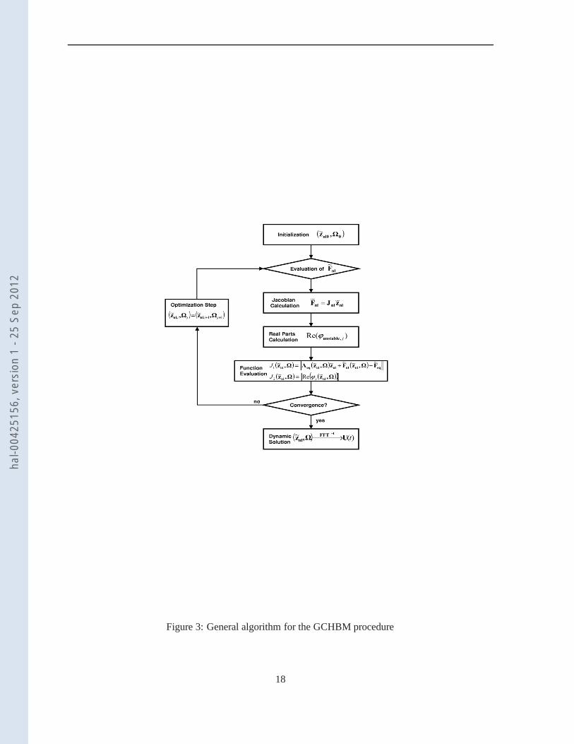
Figure 3: General algorithm for the GCHBM procedure
18
hal-0
0425
156,
ver
sion
1 -
25 S
ep 2
012
−2 −1 0 1 2 3 4−2
−1
0
1
2
3
4
k1
k 2
Figure 4: Harmonics components forp = 2 andNh = 3
19
hal-0
0425
156,
ver
sion
1 -
25 S
ep 2
012
a b
1 1.5 2 2.5 3
x 10−3
−8
−6
−4
−2
0
2
4
6
8
Displacement (m)
Vel
ocity
(m
.s−
1 )
1 1.5 2 2.5 3
x 10−3
−8
−6
−4
−2
0
2
4
6
8
Displacement (m)
Vel
ocity
(m
.s−
1 )
c d
7 7.5 8 8.5 9 9.5
x 10−3
−8
−6
−4
−2
0
2
4
6
8
Displacement (m)
Vel
ocity
(m
.s−
1 )
7 7.5 8 8.5 9 9.5
x 10−3
−8
−6
−4
−2
0
2
4
6
8
Displacement (m)
Vel
ocity
(m
.s−
1 )
e f
0.95 1 1.05 1.1 1.15
x 10−3
−0.8
−0.6
−0.4
−0.2
0
0.2
0.4
0.6
0.8
Displacement (m)
Vel
ocity
(m
.s−
1 )
0.95 1 1.05 1.1 1.15
x 10−3
−0.8
−0.6
−0.4
−0.2
0
0.2
0.4
0.6
0.8
Displacement (m)
Vel
ocity
(m
.s−
1 )
g h
−5 −4.5 −4 −3.5 −3 −2.5 −2 −1.5
x 10−5
−0.15
−0.1
−0.05
0
0.05
0.1
Displacement (m)
Vel
ocity
(m
.s−
1 )
−5 −4.5 −4 −3.5 −3 −2.5 −2 −1.5
x 10−5
−0.15
−0.1
−0.05
0
0.05
0.1
Displacement (m)
Vel
ocity
(m
.s−
1 )
Figure 5: Limit cycles forµ = 0.29. (a,b,c,d) Pad node: (a,c) GCHBM withNh = 3, (b,d) TimeIntegration; (e,f,g,h) Disc node: (e,g) GCHBM withNh = 3, (f,h) Time Integration
20
hal-0
0425
156,
ver
sion
1 -
25 S
ep 2
012
a b
0 1000 2000 3000 4000 5000
10−8
10−7
10−6
10−5
10−4
10−3
Frequency (Hz)
Pow
er S
pect
rum
Den
sity
f1 f
2
f2−f
1
2f1−f
2
2f2−2f
1
2f1
f1+f
2
2f2+f
1
2f2
3f1
3f2
2f2−f
1 2f1+f
2
0 1000 2000 3000 4000 5000
10−8
10−6
10−4
Frequency (Hz)
Pow
er S
pect
rum
Den
sity
2f1+f
2
2f2−f
1
3f2
3f1
2f2 2f
2+f
1
f1+f
2
2f12f
2−2f
1
2f1−f
2
f2−f
1
f2
f1
Figure 6: Power Spectrum Density forµ = 0.29 with Nh = 3. (a) Pad node: - - GCHBM, — TimeIntegration; (b) Disc node: - - GCHBM, — Time Integration
21
hal-0
0425
156,
ver
sion
1 -
25 S
ep 2
012
a b
1.6 1.8 2 2.2 2.4 2.6 2.8
x 10−3
−6
−4
−2
0
2
4
6
Displacement (m)
Vel
ocity
(m
.s−
1 )
1.6 1.8 2 2.2 2.4 2.6 2.8
x 10−3
−6
−4
−2
0
2
4
6
Displacement (m)
Vel
ocity
(m
.s−
1 )
c d
8 8.2 8.4 8.6 8.8 9 9.2
x 10−3
−4
−3
−2
−1
0
1
2
3
4
Displacement (m)
Vel
ocity
(m
.s−
1 )
8 8.2 8.4 8.6 8.8 9 9.2
x 10−3
−4
−3
−2
−1
0
1
2
3
4
Displacement (m)
Vel
ocity
(m
.s−
1 )
e f
0.94 0.96 0.98 1 1.02 1.04 1.06 1.08 1.1
x 10−3
−0.6
−0.4
−0.2
0
0.2
0.4
0.6
Displacement (m)
Vel
ocity
(m
.s−
1 )
0.94 0.96 0.98 1 1.02 1.04 1.06 1.08 1.1
x 10−3
−0.6
−0.4
−0.2
0
0.2
0.4
0.6
Displacement (m)
Vel
ocity
(m
.s−
1 )
g h
−5.5 −5 −4.5 −4 −3.5 −3
x 10−5
−0.1
−0.05
0
0.05
0.1
Displacement (m)
Vel
ocity
(m
.s−
1 )
−5.5 −5 −4.5 −4 −3.5 −3
x 10−5
−0.1
−0.05
0
0.05
0.1
Displacement (m)
Vel
ocity
(m
.s−
1 )
Figure 7: Limit cycles forµ = 0.35. (a,b,c,d) Pad node: (a,c) GCHBM withNh = 3, (b,d) TimeIntegration; (e,f,g,h) Disc node: (e,g) GCHBM withNh = 3, (f,h) Time Integration
22
hal-0
0425
156,
ver
sion
1 -
25 S
ep 2
012
a b
1000 2000 3000 4000 5000
10−7
10−6
10−5
10−4
10−3
10−2
Frequency (Hz)
Pow
er S
pect
rum
Den
sity
2f1+f
2
2f2−f
1
5f1
3f1
2f2
f1+2f
2
f1+f
2
2f1
2f2−2f
12f1−f
2
f2−f
1
f2
f1
3f2
3f1+f
2
4f1 2f
1+2f
2
7f1−f
2
0 1000 2000 3000 4000 500010
−8
10−7
10−6
10−5
10−4
10−3
Frequency (Hz)
Pow
er S
pect
rum
Den
sity
f1
f2
f2−f
1
2f1−f
2
2f2−2f
1
2f1
f1+f
2
f1+2f
2
2f2
3f1
(3f2)
2f2−f
1 2f1+f
2 4f1
3f1+f
2
Figure 8: Power Spectrum Density forµ = 0.35 with Nh = 3. (a) Pad node: - - GCHBM, — TimeIntegration; (b) Disc node: - - GCHBM, — Time Integration
23
hal-0
0425
156,
ver
sion
1 -
25 S
ep 2
012
a b
1 1.5 2 2.5 3
x 10−3
−8
−6
−4
−2
0
2
4
6
8
Displacement (m)
Vel
ocity
(m
.s−
1 )
1 1.5 2 2.5 3
x 10−3
−8
−6
−4
−2
0
2
4
6
8
Displacement (m)
Vel
ocity
(m
.s−
1 )
c d
0.95 1 1.05 1.1 1.15
x 10−3
−0.8
−0.6
−0.4
−0.2
0
0.2
0.4
0.6
0.8
Displacement (m)
Vel
ocity
(m
.s−
1 )
0.95 1 1.05 1.1 1.15
x 10−3
−0.8
−0.6
−0.4
−0.2
0
0.2
0.4
0.6
0.8
Displacement (m)
Vel
ocity
(m
.s−
1 )
Figure 9: Limit cycles forµ = 0.29 andNh = 2. (a,b) Pad node: (a) GCHBM, (b) Time Integration;(c,d) Disc node: (c) GCHBM, (d) Time Integration
24
hal-0
0425
156,
ver
sion
1 -
25 S
ep 2
012
a b
0 1000 2000 3000 4000 5000
10−8
10−7
10−6
10−5
10−4
10−3
Frequency (Hz)
Pow
er S
pect
rum
Den
sity
f1
2f2
2f1
f2−f
1
f1+f
2
f2
0 1000 2000 3000 4000 5000
10−8
10−6
10−4
Frequency (Hz)
Pow
er S
pect
rum
Den
sity f
1+f
2
f2−f
1
2f1
2f2
f1
f2
Figure 10: Power Spectrum Density forµ = 0.29 andNh = 2. (a) Pad node: - - GCHBM, — TimeIntegration; (b) Disc node: - - GCHBM, — Time Integration
a b
0 5 10 150
500
1000
1500
2000
2500
3000
3500
4000
4500
Iterations
Nor
m o
f the
Res
idue
0 5 10 15−10
−5
0
5
10
15
20
25
30
35
Iterations
Evo
lutio
n of
Rea
l Par
ts
Figure 11: Evolution of parameters with iterations (Nh = 2, µ = 0.29). (a) Norm of Residue; (b) RealParts: —1st mode, -.-2nd mode
25
hal-0
0425
156,
ver
sion
1 -
25 S
ep 2
012
a b
0 1000 2000 3000 4000 5000
10−15
10−10
10−5
Frequency (Hz)
Pow
er S
pect
rum
Den
sity
f1
2f2−2f
1
f2−f
1
2f1−f
2
f2
2f1
2f2−f
1
f1+f
2
3f1
2f22f
1+f
2
2f2+f
1
3f2
4f1
3f1+f
2
2f1+2f
2
0 1000 2000 3000 4000 5000
10−8
10−6
10−4
Frequency (Hz)
Pow
er S
pect
rum
Den
sity
2f1+2f
2
3f1+f
2
4f1
3f2
2f2+f
1
2f1+f
2
2f2
3f1
f1+f
2
2f2−f
1
2f1
f2
2f1−f
2
f2−f
1
2f2−2f
1
f1
Figure 12: Power Spectrum Density forµ = 0.29 with Nh = 5. (a) Pad node: - - GCHBM, — TimeIntegration; (b) Disc node: - - GCHBM, — Time Integration
26
hal-0
0425
156,
ver
sion
1 -
25 S
ep 2
012
a b
1.6 1.8 2 2.2 2.4 2.6 2.8
x 10−3
−5
−4
−3
−2
−1
0
1
2
3
4
5
Displacement (m)
Vel
ocity
(m
.s−
1 )
1.6 1.8 2 2.2 2.4 2.6 2.8
x 10−3
−6
−4
−2
0
2
4
6
Displacement (m)
Vel
ocity
(m
.s−
1 )
c d
0.95 1 1.05 1.1
x 10−3
−0.6
−0.4
−0.2
0
0.2
0.4
0.6
Displacement (m)
Vel
ocity
(m
.s−
1 )
0.94 0.96 0.98 1 1.02 1.04 1.06 1.08 1.1
x 10−3
−0.6
−0.4
−0.2
0
0.2
0.4
0.6
Displacement (m)
Vel
ocity
(m
.s−
1 )
Figure 13: Limit cycles forµ = 0.35 andNh = 2. (a,b) Pad node: (a) GCHBM, (b) Time Integration;(c,d) Disc node: (c) GCHBM, (d) Time Integration
27
hal-0
0425
156,
ver
sion
1 -
25 S
ep 2
012

a b
0 1000 2000 3000 4000 5000
10−8
10−6
10−4
Frequency (Hz)
Pow
er S
pect
rum
Den
sity
f1 f
2
f2−f
1
2f1
f1+f
2
2f2
0 1000 2000 3000 4000 5000
10−8
10−6
10−4
Frequency (Hz)
Pow
er S
pect
rum
Den
sity
f1
f2
f2−f
1
2f1
f1+f
2
2f2
Figure 14: Power Spectrum Density forµ = 0.35 andNh = 2. (a) Pad node: - - GCHBM, — TimeIntegration; (b) Disc node: - - GCHBM, — Time Integration
28
hal-0
0425
156,
ver
sion
1 -
25 S
ep 2
012
a b
2.1 2.2 2.3 2.4 2.5 2.6 2.7 2.8
x 10−3
−3
−2
−1
0
1
2
3
4
Displacement (m)
Vel
ocity
(m
.s−
1 )
8.6 8.7 8.8 8.9 9 9.1
x 10−3
−2
−1.5
−1
−0.5
0
0.5
1
1.5
2
Displacement (m)
Vel
ocity
(m
.s−
1 )
c d
1 1.01 1.02 1.03 1.04
x 10−3
−0.2
−0.15
−0.1
−0.05
0
0.05
0.1
0.15
0.2
0.25
Displacement (m)
Vel
ocity
(m
.s−
1 )
−6.5 −6 −5.5 −5 −4.5
x 10−5
−0.1
−0.05
0
0.05
0.1
0.15
Displacement (m)
Vel
ocity
(m
.s−
1 )
Figure 15: Limit cycles forµ = 0.40. (a,b) Pad node: - - GCHBM, — Time Integration; (c,d) Discnode:- - GCHBM, — Time Integration
29
hal-0
0425
156,
ver
sion
1 -
25 S
ep 2
012
a b
0 1000 2000 3000 4000 5000
10−8
10−6
10−4
Frequency (Hz)
Pow
er S
pect
rum
Den
sity
f1 2f
1 3f1
0 1000 2000 3000 4000 5000
10−8
10−6
10−4
Frequency (Hz)
Pow
er S
pect
rum
Den
sity
f1
2f1
3f1
Figure 16: Power Spectrum Density forµ = 0.40. (a) Pad node: - - GCHBM, — Time Integration; (b)Disc node: - - GCHBM, — Time Integration
30
hal-0
0425
156,
ver
sion
1 -
25 S
ep 2
012
7 7.5 8 8.5 9 9.5
x 10−3
−8
−6
−4
−2
0
2
4
6
8
Displacement (m)
Vel
ocity
(m
.s−
1 )
7.5 8 8.5 9 9.5
x 10−3
−8
−6
−4
−2
0
2
4
6
8
Displacement (m)
Vel
ocity
(m
.s−
1 )
7.5 8 8.5 9 9.5
x 10−3
−6
−4
−2
0
2
4
6
8
Displacement (m)
Vel
ocity
(m
.s−
1 )
7.5 8 8.5 9 9.5
x 10−3
−6
−4
−2
0
2
4
6
Displacement (m)
Vel
ocity
(m
.s−
1 )
µ = 0.29 µ = 0.30 µ = 0.31 µ = 0.32
8 8.5 9 9.5
x 10−3
−6
−4
−2
0
2
4
6
Displacement (m)
Vel
ocity
(m
.s−
1 )
8 8.5 9
x 10−3
−4
−2
0
2
4
6
Displacement (m)
Vel
ocity
(m
.s−
1 )
8 8.2 8.4 8.6 8.8 9 9.2
x 10−3
−4
−3
−2
−1
0
1
2
3
4
Displacement (m)
Vel
ocity
(m
.s−
1 )
8.2 8.4 8.6 8.8 9
x 10−3
−3
−2
−1
0
1
2
3
Displacement (m)
Vel
ocity
(m
.s−
1 )
µ = 0.33 µ = 0.34 µ = 0.35 µ = 0.355
8.3 8.4 8.5 8.6 8.7 8.8 8.9 9 9.1
x 10−3
−2.5
−2
−1.5
−1
−0.5
0
0.5
1
1.5
2
2.5
Displacement (m)
Vel
ocity
(m
.s−
1 )
8.4 8.5 8.6 8.7 8.8 8.9 9 9.1
x 10−3
−2.5
−2
−1.5
−1
−0.5
0
0.5
1
1.5
2
Displacement (m)
Vel
ocity
(m
.s−
1 )
8.6 8.7 8.8 8.9 9 9.1
x 10−3
−2
−1.5
−1
−0.5
0
0.5
1
1.5
2
Displacement (m)
Vel
ocity
(m
.s−
1 )
8.7 8.75 8.8 8.85 8.9 8.95 9 9.05 9.1
x 10−3
−2
−1.5
−1
−0.5
0
0.5
1
1.5
Displacement (m)
Vel
ocity
(m
.s−
1 )
µ = 0.36 µ = 0.38 µ = 0.40 µ = 0.44
8.8 8.85 8.9 8.95 9 9.05 9.1 9.15
x 10−3
−1.5
−1
−0.5
0
0.5
1
1.5
Displacement (m)
Vel
ocity
(m
.s−
1 )
8.85 8.9 8.95 9 9.05 9.1 9.15 9.2 9.25
x 10−3
−2
−1.5
−1
−0.5
0
0.5
1
1.5
Displacement (m)
Vel
ocity
(m
.s−
1 )
9 9.1 9.2 9.3
x 10−3
−2
−1
0
1
2
Displacement (m)
Vel
ocity
(m
.s−
1 )
9 9.1 9.2 9.3 9.4
x 10−3
−2.5
−2
−1.5
−1
−0.5
0
0.5
1
1.5
2
2.5
Displacement (m)
Vel
ocity
(m
.s−
1 )
µ = 0.48 µ = 0.52 µ = 0.56 µ = 0.60
Figure 17: Limit cycles from the GCHBM with varying frictioncoefficientµ
31
hal-0
0425
156,
ver
sion
1 -
25 S
ep 2
012
0.3 0.4 0.5 0.6 0.7 0.8 0.90
5
10
15
Friction Coefficient
α 1/α2
Figure 18: Propensity index ratioα1/α2 versusµ. The dotted line indicates the transition from two toone unstable mode in the dynamic steady-state.
32
hal-0
0425
156,
ver
sion
1 -
25 S
ep 2
012
a b
0.29 0.3 0.31 0.32 0.33 0.34 0.35
898
900
902
904
Friction Coefficient
Fre
quen
cies
(H
z)
0.29 0.3 0.31 0.32 0.33 0.34 0.35
1495.5
1496
1496.5
1497
Friction Coefficient
Fre
quen
cies
(H
z)
0.4 0.45 0.5 0.55 0.6 0.65
865
870
875
880
885
890
895
900
Friction Coefficient
Fre
quen
cies
(H
z)
c
0.3 0.35 0.4 0.45 0.5 0.55 0.6 0.65
6.55
6.6
6.65
6.7
6.75
6.8
6.85
6.9
6.95
x 10−4
Friction Coefficient
Tot
al A
mpl
itude
Ene
rgy
Figure 19: Evolution of parameters withµ. (a) Both unstable modes,0.29 < µ < 0.36; (b) First unstablemode0.36 < µ < 0.68; (c) Total amplitude energy,0.29 < µ < 0.68
33
hal-0
0425
156,
ver
sion
1 -
25 S
ep 2
012
a b
0 5 10 15 20 25 30 35
−5
0
5
10
15
Iterations
Evo
lutio
n of
Rea
l Par
ts
0 5 10 15 20 25 30 35−20
−18
−16
−14
−12
−10
−8
−6
−4
−2
0
Iterations
∆ f (
Hz)
c
0 5 10 15 20 25 30 350
500
1000
1500
2000
2500
3000
3500
4000
Iterations
Nor
m o
f the
Res
idue
Figure 20: Evolution of parameters with iterations (µ = 0.29). (a) Real Parts: —1st mode, -.-2nd mode;(b) Frequencies: —1st mode, -.-2nd mode; (c) Norm of Residue
34
hal-0
0425
156,
ver
sion
1 -
25 S
ep 2
012
Recommended


