Simple harmonic motion

March 24, 2016

An account is given for the simplest kind of oscil-latory motion, due to a linear restoring force andwithout dissipation or external driving. An infor-mal approach is taken for the mathematics, witha more systematic account of ordinary differentialequations given in the next module.

Contents

1 Introduction and kinematics 11.1 Canonical model and basic properties 11.2 Simple harmonic motion . . . . . . . 21.3 Velocity and acceleration . . . . . . . 21.4 Graphical representation . . . . . . . 21.5 Complex representation . . . . . . . 3

2 Solving equation of motion 32.1 Equation of motion . . . . . . . . . . 32.2 Solution in polar form . . . . . . . . 42.3 Solution in alternate form . . . . . . 42.4 Matching initial conditions . . . . . 5

3 Adding a constant force 53.1 The generalized model . . . . . . . . 53.2 Shifting the origin . . . . . . . . . . 53.3 The potential energy . . . . . . . . . 6

4 The generality of SHM 64.1 Small oscillations about equilibrium 6

1 Introduction and kinemat-ics

1.1 Canonical model and basic prop-erties

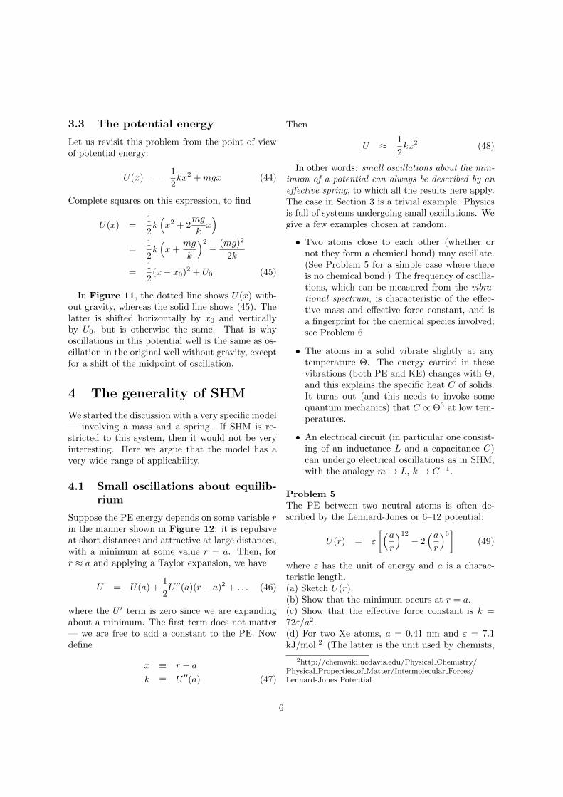
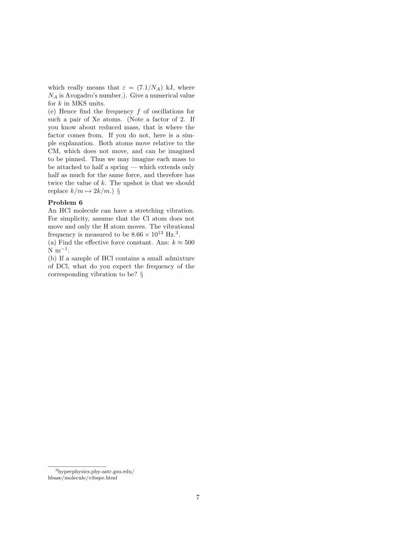
Canonical modelWe first define the simplest model of an oscillat-ing system and describe the motion. A mass m isattached to a spring with force constant k (Fig-ure 1). Although the system is shown vertically(for convenience in some diagrams, e.g., Figure 2below), it is assumed there is no gravity; that ad-ditional feature will be discussed in Section 3. Themass is given an initial displacement x(0) (mea-sured from the neutral position of the spring) andan initial velocity v(0). Its subsequent motion issketched versus time t in Figure 2, for the casex(0) > 0 and v(0) = 0.

PeriodThe mass oscillates back and forth, and the motionrepeats in a time T , called the period (Figure 3)— the time between successive peaks, and moregenerally the time between corresponding points inthe motion. Periodicity is expressed precisely as

x(t+ T ) = x(t) (1)

for any t.The number of oscillations per unit time is the

frequency f . Since there is one complete oscillationper time interval T , the frequency is

f =1

T(2)

The unit of frequency is s−1 = Hz.

AmplitudeThe oscillation has an amplitude A (Figure 3).

1

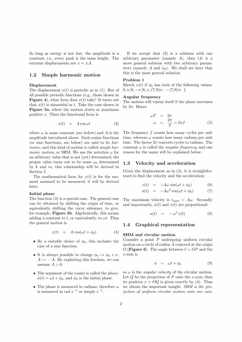
So long as energy is not lost, the amplitude is aconstant, i.e., every peak is the same height. Theextreme displacements are x = ±A.

1.2 Simple harmonic motion

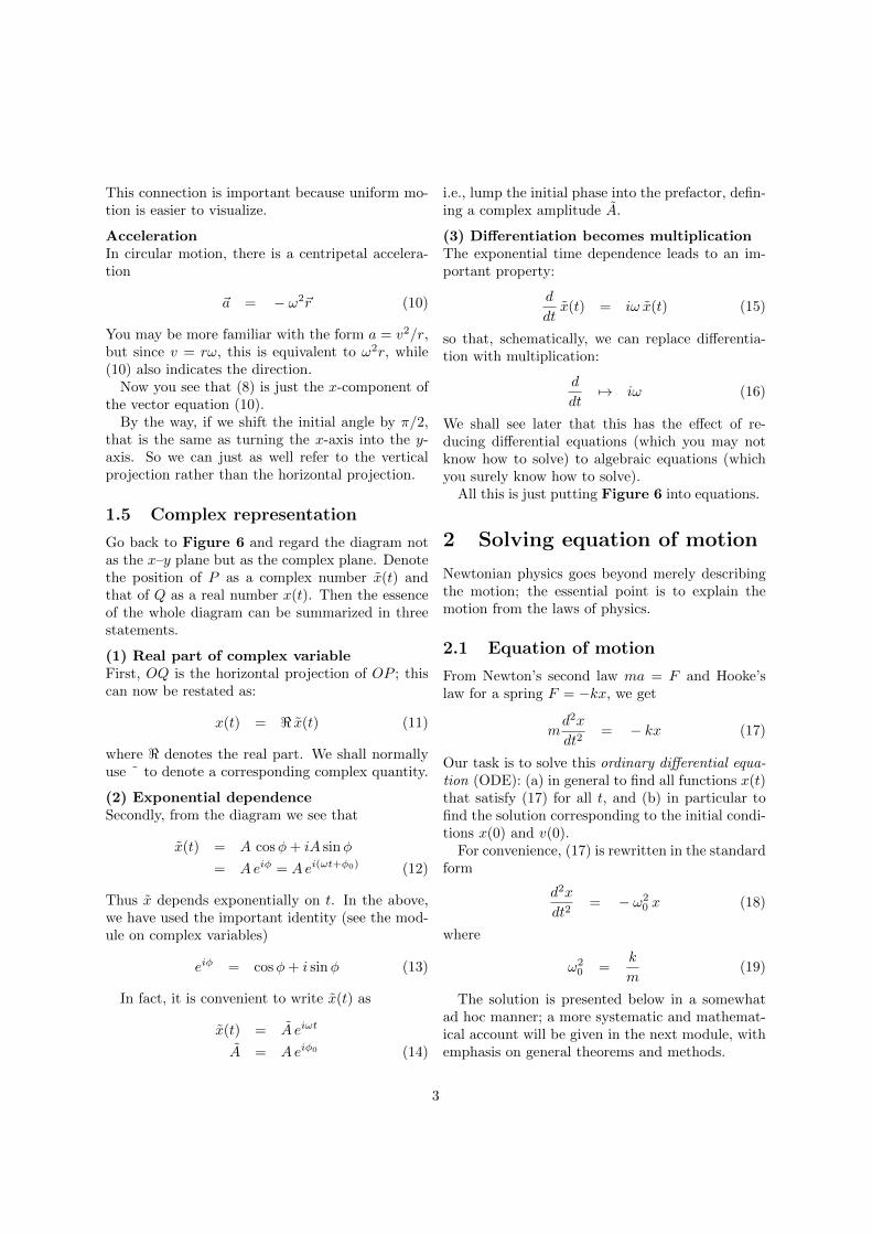
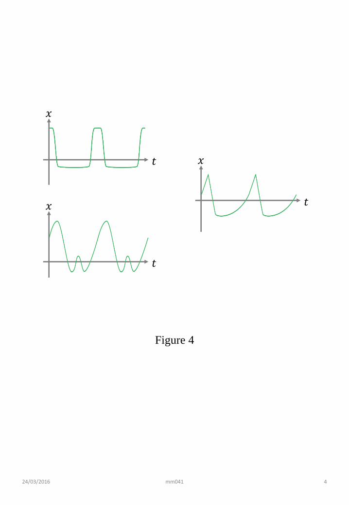
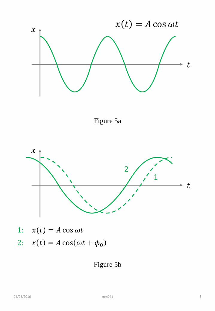
DisplacementThe displacement x(t) is periodic as in (1). But ofall possible periodic functions (e.g., those shown inFigure 4), what form does x(t) take? It turns outthat x(t) is sinusoidal in t. Take the case shown inFigure 5a, where the motion starts at maximumpositive x. Then the functional form is

x(t) = A cosωt (3)

where ω is some constant (see below) and A is theamplitude introduced above. Such cosine functions(or sine functions; see below) are said to be har-monic, and this kind of motion is called simple har-monic motion, or SHM. We use the notation ω foran arbitrary value that is not (yet) determined; theproper value turns out to be some ω0 determinedby k and m; this relationship will be derived inSection 2.

The mathematical form for x(t) is for the mo-ment assumed to be measured; it will be derivedlater.

Initial phaseThe function (3) is a special case. The general casecan be obtained by shifting the origin of time, orequivalently shifting the curve sideways, to give,for example, Figure 5b. Algebraically, this meansadding a constant to t, or equivalently, to ωt. Thusthe general motion is

x(t) = A cos(ωt+ φ0) (4)

• By a suitable choice of φ0, this includes thecase of a sine function.

• It is always possible to change φ0 7→ φ0 + π,A 7→ −A. By exploiting this freedom, we canassume A > 0.

• The argument of the cosine is called the phase:φ(t) = ωt+ φ0, and φ0 is the initial phase.

• The phase is measured in radians; therefore ωis measured in rad s−1 or simply s−1.

If we accept that (3) is a solution with onearbitrary parameter (namely A), then (4) is amore general solution with two arbitrary param-eters (namely A and φ0). We shall see later thatthis is the most general solution.

Problem 1Sketch x(t) if φ0 has each of the following values:0, π/6,−π/6, π, (7/6)π, − (7/6)π. §

Angular frequencyThe motion will repeat itself if the phase increasesby 2π. Hence

ωT = 2π

ω =2π

T= 2πf (5)

The frequency f counts how many cycles per unittime, whereas ω counts how many radians per unittime. The factor 2π converts cycles to radians. Theconstant ω is called the angular frequency, and onereason for the name will be explained below.

1.3 Velocity and acceleration

Given the displacement as in (4), it is straightfor-ward to find the velocity and the acceleration:

v(t) = −Aω sin(ωt+ φ0) (6)

a(t) = −Aω2 cos(ωt+ φ0) (7)

The maximum velocity is vmax = Aω. Secondlyand importantly, a(t) and x(t) are proportional:

a(t) = − ω2 x(t) (8)

1.4 Graphical representation

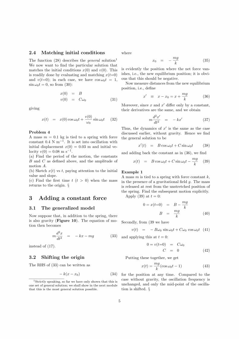
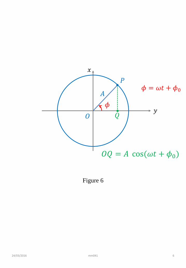
SHM and circular motionConsider a point P undergoing uniform circularmotion on a circle of radius A centered at the originO (Figure 6). The angle between ~r = OP and thex-axis is

φ = ωt+ φ0 (9)

so ω is the angular velocity of the circular motion.Let Q be the projection of P onto the x-axis; thenits position x = OQ is given exactly by (4). Thuswe obtain the important insight: SHM is the pro-jection of uniform circular motion onto one axis.

2

This connection is important because uniform mo-tion is easier to visualize.

AccelerationIn circular motion, there is a centripetal accelera-tion

~a = − ω2~r (10)

You may be more familiar with the form a = v2/r,but since v = rω, this is equivalent to ω2r, while(10) also indicates the direction.

Now you see that (8) is just the x-component ofthe vector equation (10).

By the way, if we shift the initial angle by π/2,that is the same as turning the x-axis into the y-axis. So we can just as well refer to the verticalprojection rather than the horizontal projection.

1.5 Complex representation

Go back to Figure 6 and regard the diagram notas the x–y plane but as the complex plane. Denotethe position of P as a complex number x(t) andthat of Q as a real number x(t). Then the essenceof the whole diagram can be summarized in threestatements.

(1) Real part of complex variableFirst, OQ is the horizontal projection of OP ; thiscan now be restated as:

x(t) = < x(t) (11)

where < denotes the real part. We shall normallyuse ˜ to denote a corresponding complex quantity.

(2) Exponential dependenceSecondly, from the diagram we see that

x(t) = A cosφ+ iA sinφ

= Aeiφ = Aei(ωt+φ0) (12)

Thus x depends exponentially on t. In the above,we have used the important identity (see the mod-ule on complex variables)

eiφ = cosφ+ i sinφ (13)

In fact, it is convenient to write x(t) as

x(t) = A eiωt

A = Aeiφ0 (14)

i.e., lump the initial phase into the prefactor, defin-ing a complex amplitude A.

(3) Differentiation becomes multiplicationThe exponential time dependence leads to an im-portant property:

d

dtx(t) = iω x(t) (15)

so that, schematically, we can replace differentia-tion with multiplication:

d

dt7→ iω (16)

We shall see later that this has the effect of re-ducing differential equations (which you may notknow how to solve) to algebraic equations (whichyou surely know how to solve).

All this is just putting Figure 6 into equations.

2 Solving equation of motion

Newtonian physics goes beyond merely describingthe motion; the essential point is to explain themotion from the laws of physics.

2.1 Equation of motion

From Newton’s second law ma = F and Hooke’slaw for a spring F = −kx, we get

md2x

dt2= − kx (17)

Our task is to solve this ordinary differential equa-tion (ODE): (a) in general to find all functions x(t)that satisfy (17) for all t, and (b) in particular tofind the solution corresponding to the initial condi-tions x(0) and v(0).

For convenience, (17) is rewritten in the standardform

d2x

dt2= − ω2

0 x (18)

where

ω20 =

k

m(19)

The solution is presented below in a somewhatad hoc manner; a more systematic and mathemat-ical account will be given in the next module, withemphasis on general theorems and methods.

3

2.2 Solution in polar form

General solution in polar formIn view of (8), it is obvious that (4) is a solution,provided the angular frequency is chosen to be ω =ω0. Thus

x(t) = A cos(ω0t+ φ0) (20)

PeriodTherefore we find that the period is given in termsof the system parameters by

T =2π

ω0= 2π

√m

k(21)

Check that the answer “makes sense”: the motionis slower (T↑) if the mass is heavier (m↑) or if thespring is weaker (k↓). The dependence (but notthe numerical prefactor) can also be obtained bydimensional analysis.

Problem 2Assume that the period for SHM with amplitude Agoes as

T = C kαmβAγ (22)

where C is a numerical constant. Use dimensionalanalysis to determine the exponents α, β, γ. §

Problem 3A mass m is subject to a restoring force that goes as−kx3. For oscillations (which would not be simpleharmonic) with amplitude A, again find the expo-nents as in (22). Note that k now has a differentmeaning and carries different units. This motioncannot be solved analytically. §

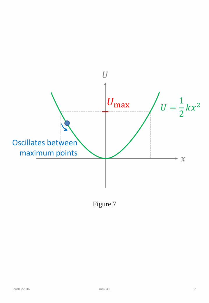
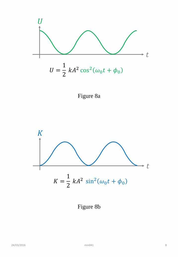
Potential energyFor a force −kx, the corresponding PE is

U(x) =1

2kx2 (23)

shown in Figure 7. The mass m oscillates in thiswell between the two extreme points shown. ThePE as a function of time is

U(t) =1

2kx(t)2

=1

2kA2 cos2(ω0t+ φ0) (24)

shown in Figure 8a.

VelocityThe velocity is given by the derivative of (20):

v(t) = −Aω0 sin(ω0t+ φ0) (25)

Kinetic energyThe KE in SHM is

K(t) =1

2mv2

=1

2m(Aω0)2 sin2(ω0t+ φ0)

=1

2kA2 sin2(ω0t+ φ0) (26)

since mω20 = k. This is shown in Figure 8b.

Conservation of energyThe total energy is therefore

E(t) = U(t) +K(t)

=1

2kA2

[cos2(ω0t+ φ0) + sin2(ω0t+ φ0)

]=

1

2kA2 (27)

independent of time, i.e., energy is conserved.

2.3 Solution in alternate form

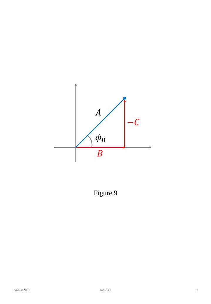
We can write the solution in a different form:

x(t) = A cos(ω0t+ φ0)

= A (cosφ0 cosω0t− sinφ0 sinω0t)

= B cosω0t+ C sinω0t (28)

where

B = A cosφ0 , C = −A sinφ0 (29)

In this representation, the solution is parameter-ized by (B,C) rather than (A, φ0). The relation-ship between these two descriptions is illustrated inFigure 9, and is like the transformation betweenpolar coordinates to Cartesian coordinates.

From (28), we find

v(t) = −Bω0 sinω0t+ Cω0 cosω0t

a(t) = −Bω20 cosω0t− Cω2

0 sinω0t (30)

4

2.4 Matching initial conditions

The function (28) describes the general solution1

We now want to find the particular solution thatmatches the initial conditions x(0) and v(0). Thisis readily done by evaluating and matching x(t=0)and v(t=0); in each case, we have cosω0t = 1,sinω0t = 0, so from (30):

x(0) = B

v(0) = Cω0 (31)

giving

x(t) = x(0) cosω0t+v(0)

ω0sinω0t (32)

Problem 4A mass m = 0.1 kg is tied to a spring with forceconstant 0.4 N m−1. It is set into oscillation withinitial displacement x(0) = 0.03 m and initial ve-locity v(0) = 0.08 m s−1.(a) Find the period of the motion, the constantsB and C as defined above, and the amplitude ofmotion A.(b) Sketch x(t) vs t, paying attention to the initialvalue and slope.(c) Find the first time t (t > 0) when the massreturns to the origin. §

3 Adding a constant force

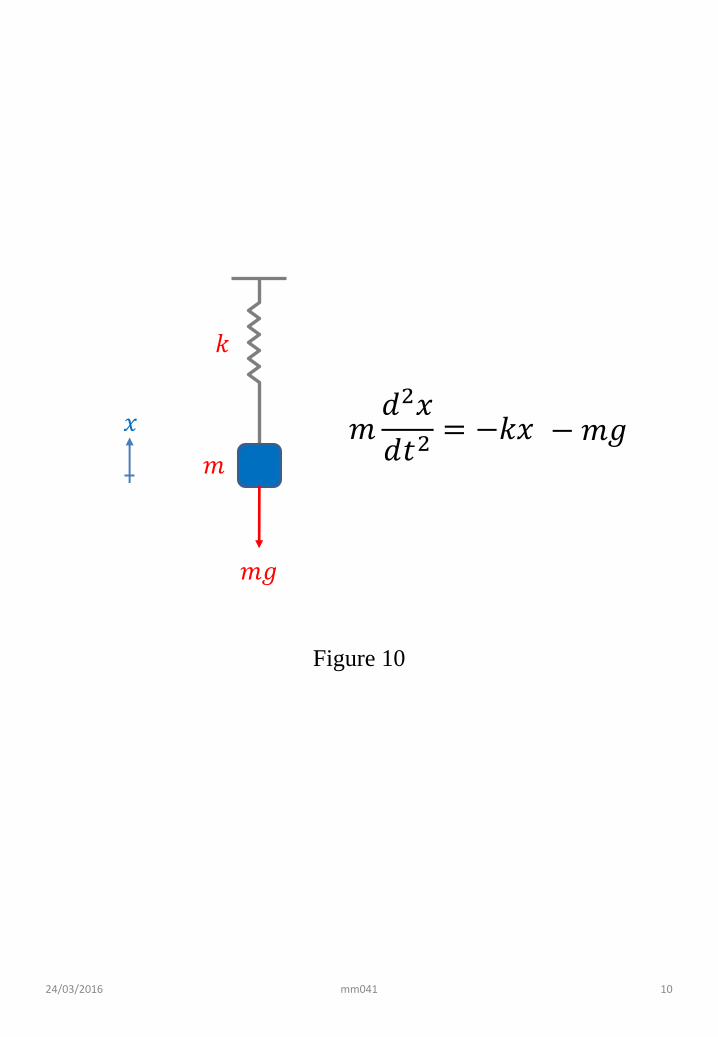
3.1 The generalized model

Now suppose that, in addition to the spring, thereis also gravity (Figure 10). The equation of mo-tion then becomes

md2x

dt2= − kx−mg (33)

instead of (17).

3.2 Shifting the origin

The RHS of (33) can be written as

− k(x− x0) (34)

1Strictly speaking, so far we have only shown that this isone set of general solution; we shall show in the next modulethat this is the most general solution possible.

where

x0 = − mg

k(35)

is evidently the position where the net force van-ishes, i.e., the new equilibrium position; it is obvi-ous that this should be negative.

Now measure distances from the new equilibriumposition, i.e., define

x′ ≡ x− x0 = x+mg

k(36)

Moreover, since x and x′ differ only by a constant,their derivatives are the same, and we obtain

md2x′

dt2= − kx′ (37)

Thus, the dynamics of x′ is the same as the casediscussed earlier, without gravity. Hence we findthe general solution to be

x′(t) = B cosω0t+ C sinω0t (38)

and adding back the constant as in (36), we find

x(t) = B cosω0t+ C sinω0t−mg

k(39)

Example 1A mass m is tied to a spring with force constant k,in the presence of a gravitational field g. The massis released at rest from the unstretched position ofthe spring. Find the subsequent motion explicitly.

Apply (39) at t = 0:

0 = x(t=0) = B − mg

k

B =mg

k(40)

Secondly, from (39 we have

v(t) = −Bω0 sinω0t+ Cω0 cosω0t (41)

and applying this at t = 0:

0 = v(t=0) = Cω0

C = 0 (42)

Putting these together, we get

x(t) =mg

k(cosω0t− 1) (43)

for the position at any time. Compared to thecase without gravity, the oscillation frequency isunchanged, and only the mid-point of the oscilla-tion is shifted. §

5

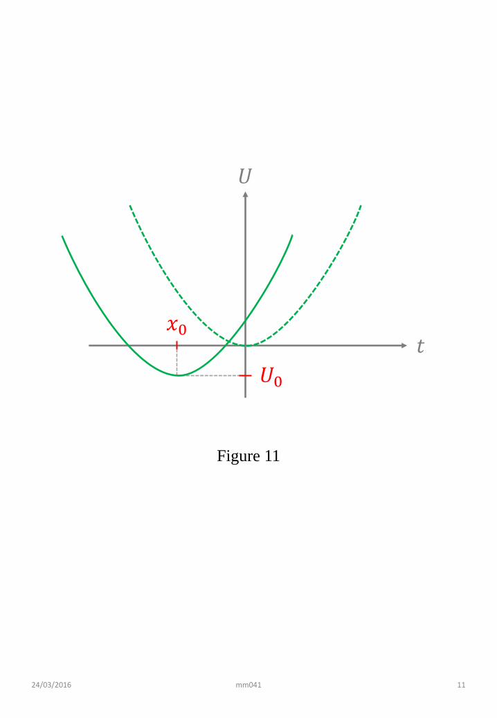
3.3 The potential energy

Let us revisit this problem from the point of viewof potential energy:

U(x) =1

2kx2 +mgx (44)

Complete squares on this expression, to find

U(x) =1

2k(x2 + 2

mg

kx)

=1

2k(x+

mg

k

)2− (mg)2

2k

=1

2(x− x0)2 + U0 (45)

In Figure 11, the dotted line shows U(x) with-out gravity, whereas the solid line shows (45). Thelatter is shifted horizontally by x0 and verticallyby U0, but is otherwise the same. That is whyoscillations in this potential well is the same as os-cillation in the original well without gravity, exceptfor a shift of the midpoint of oscillation.

4 The generality of SHM

We started the discussion with a very specific model— involving a mass and a spring. If SHM is re-stricted to this system, then it would not be veryinteresting. Here we argue that the model has avery wide range of applicability.

4.1 Small oscillations about equilib-rium

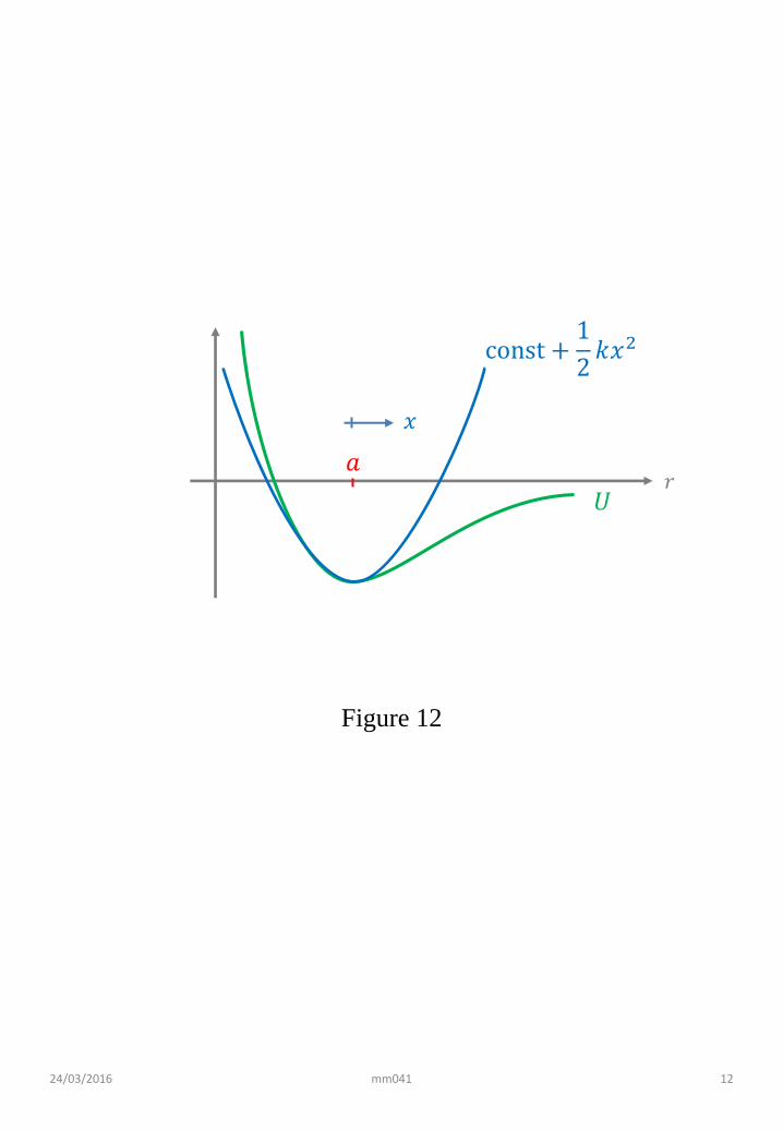
Suppose the PE energy depends on some variable rin the manner shown in Figure 12: it is repulsiveat short distances and attractive at large distances,with a minimum at some value r = a. Then, forr ≈ a and applying a Taylor expansion, we have

U = U(a) +1

2U ′′(a)(r − a)2 + . . . (46)

where the U ′ term is zero since we are expandingabout a minimum. The first term does not matter— we are free to add a constant to the PE. Nowdefine

x ≡ r − ak ≡ U ′′(a) (47)

Then

U ≈ 1

2kx2 (48)

In other words: small oscillations about the min-imum of a potential can always be described by aneffective spring, to which all the results here apply.The case in Section 3 is a trivial example. Physicsis full of systems undergoing small oscillations. Wegive a few examples chosen at random.

• Two atoms close to each other (whether ornot they form a chemical bond) may oscillate.(See Problem 5 for a simple case where thereis no chemical bond.) The frequency of oscilla-tions, which can be measured from the vibra-tional spectrum, is characteristic of the effec-tive mass and effective force constant, and isa fingerprint for the chemical species involved;see Problem 6.

• The atoms in a solid vibrate slightly at anytemperature Θ. The energy carried in thesevibrations (both PE and KE) changes with Θ,and this explains the specific heat C of solids.It turns out (and this needs to invoke somequantum mechanics) that C ∝ Θ3 at low tem-peratures.

• An electrical circuit (in particular one consist-ing of an inductance L and a capacitance C)can undergo electrical oscillations as in SHM,with the analogy m 7→ L, k 7→ C−1.

Problem 5The PE between two neutral atoms is often de-scribed by the Lennard-Jones or 6–12 potential:

U(r) = ε

[(ar

)12− 2

(ar

)6](49)

where ε has the unit of energy and a is a charac-teristic length.(a) Sketch U(r).(b) Show that the minimum occurs at r = a.(c) Show that the effective force constant is k =72ε/a2.(d) For two Xe atoms, a = 0.41 nm and ε = 7.1kJ/mol.2 (The latter is the unit used by chemists,

2http://chemwiki.ucdavis.edu/Physical Chemistry/Physical Properties of Matter/Intermolecular Forces/Lennard-Jones Potential

6

which really means that ε = (7.1/NA) kJ, whereNA is Avogadro’s number.). Give a numerical valuefor k in MKS units.(e) Hence find the frequency f of oscillations forsuch a pair of Xe atoms. (Note a factor of 2. Ifyou know about reduced mass, that is where thefactor comes from. If you do not, here is a sim-ple explanation. Both atoms move relative to theCM, which does not move, and can be imaginedto be pinned. Thus we may imagine each mass tobe attached to half a spring — which extends onlyhalf as much for the same force, and therefore hastwice the value of k. The upshot is that we shouldreplace k/m 7→ 2k/m.) §

Problem 6An HCl molecule can have a stretching vibration.For simplicity, assume that the Cl atom does notmove and only the H atom moves. The vibrationalfrequency is measured to be 8.66× 1013 Hz.3.(a) Find the effective force constant. Ans: k ≈ 500N m−1.(b) If a sample of HCl contains a small admixtureof DCl, what do you expect the frequency of thecorresponding vibration to be? §

3hyperphysics.phy-astr.gsu.edu/hbase/molecule/vibspe.html

7

24/03/2016 mm041 1

𝑘

𝑚

Figure 1

24/03/2016 mm041 2

𝑥

𝑡

Figure 2

24/03/2016 mm041 3

𝑥

𝑡

𝑇

Figure 3

Amplitude

Period

𝐴

24/03/2016 mm041 4

𝑥

𝑡𝑥

𝑡

𝑥

𝑡

Figure 4

24/03/2016 mm041 5

𝑥

𝑡

𝑥 𝑡 = 𝐴 cos𝜔𝑡

𝑥

𝑡

𝑥 𝑡 = 𝐴 cos𝜔𝑡

𝑥 𝑡 = 𝐴 cos 𝜔𝑡 + 𝜙0

12

1:

2:

Figure 5a

Figure 5b

24/03/2016 mm041 6

𝑂𝑄 = 𝐴 cos(𝜔𝑡 + 𝜙0)

𝑃

𝐴

𝑂 𝑄

𝜙 = 𝜔𝑡 + 𝜙0

𝜙

𝑥

𝑦

Figure 6

24/03/2016 mm041 7

Figure 7

𝑈

𝑥

𝑈 =1

2𝑘𝑥2

𝑈max

Oscillates between maximum points

24/03/2016 mm041 8

𝐾

𝑡

𝐾 =1

2𝑘𝐴2 sin2 𝜔0𝑡 + 𝜙0

𝑈 =1

2𝑘𝐴2 cos2 𝜔0𝑡 + 𝜙0

𝑈

𝑡

Figure 8a

Figure 8b

24/03/2016 mm041 9

𝐵

𝐴−𝐶

𝜙0

Figure 9

24/03/2016 mm041 10

𝑘

𝑚

𝑚𝑑2𝑥

𝑑𝑡2= −𝑘𝑥

𝑚𝑔

𝑥 −𝑚𝑔

Figure 10

24/03/2016 mm041 11

𝑈

𝑡𝑥0

𝑈0

Figure 11

24/03/2016 mm041 12

𝑈𝑟

𝑎

𝑥

const +1

2𝑘𝑥2

Figure 12