Estuarine, Coastal and Shelf Science 68 (2006) 1e16www.elsevier.com/locate/ecss

Storm tide simulation in the Chesapeake Bayusing an unstructured grid model

Jian Shen*, Harry Wang, Mac Sisson, Wenping Gong

Virginia Institute of Marine Science, The College of William and Mary, The School of Marine Science, P.O. Box 1346, Gloucester Point, VA 23062, USA

Received 29 November 2004; accepted 7 December 2005

Available online 18 April 2006

Abstract

Hurricane Isabel made landfall near Drum Inlet, North Carolina on September 18, 2003 (UTC 17:00). Although it was classified as only aCategory 2 storm (SaffireSimpson scale), Hurricane Isabel had a significant impact on the Chesapeake Bay with a 1.5e2.0 m storm surge(above mean sea level), and was dubbed the ‘‘100-year storm’’. A high-resolution unstructured grid model (UnTRIM) was applied to simulatestorm tide in the Chesapeake Bay. The application of an unstructured grid in the Bay offers the greatest flexibilities in representing complexestuarine geometry near the coast and encompassing a large modeling domain necessary for storm surge simulation. The resulting mesh hasa total of 239,541 surface elements. The model was forced by 9 tidal harmonic constituents at the open boundary and a wind field generatedby a parametric wind model. A hindcast simulation of Hurricane Isabel captures both peak storm tide and surge evolution in various sites of theBay. Model diagnostic studies indicate that the high surge occurring in the upper Bay regions was mainly caused by the forced southerly wind,whereas the offshore surge and both the northeasterly and southeasterly winds influenced the lower Bay region more significantly.� 2006 Elsevier Ltd. All rights reserved.

Keywords: storm surge; unstructured grid model; UnTRIM; Isabel; Chesapeake Bay

1. Introduction

Numerical model predictions of coastal storm surge haveplayed an important role in coastal engineering design, disas-ter planning and mitigation, and coastal management. Manymodels have been developed for the simulation of storm surgesin the last decade (Lynch, 1983; Blumberg and Mellor, 1987;Flather et al., 1991; Jelesnianski et al., 1992; Luettich et al.,1992; Verboom et al., 1992; Westerink et al., 1992; Hubbertand McInnes, 1999). Recently, modeling operational systems,such as the storm tide warning service in the U.K. (Proctor andFlather, 1983; Flather et al., 1991), the real time storm surgeforecasting system in the Netherlands (DeVries, 1991; Gerrit-sen et al., 1995), and the surge warning system for the NorthSea (Vested et al., 1992), have been developed and improved

* Corresponding author.

E-mail address: shen@vims.edu (J. Shen).

0272-7714/$ - see front matter � 2006 Elsevier Ltd. All rights reserved.

doi:10.1016/j.ecss.2005.12.018

in Western Europe. Current publications indicate a renewedinterest in storm surge modeling (Bode and Hardy, 1997).

Storm surge is a long-period wave caused by extreme windand pressure force. The intensity of storm surge and its impacton the coastal regions depend on the intensity of forcing andthe path of the storm, characteristics of bathymetry, and geo-metric properties of a waterbody. Three factors are importantwhen developing a storm surge model at any particular loca-tion: (1) the adequacy of the grid resolution; (2) the specifica-tion of boundary conditions; and (3) the representation ofresonant modes and surge frequency (Reid, 1990).

Adequacy of the grid resolution is crucial for predictingnearshore storm tide and flooding accurately. To improve sim-ulation accuracy, a small grid cell size is needed for shallowwater regions and low-lying areas to resolve complex topo-graphic and bathymetric features. Many previous model appli-cations suggest that a much higher level of grid detail isrequired if nearshore tidal currents are to be considered

2 J. Shen et al. / Estuarine, Coastal and Shelf Science 68 (2006) 1e16

(Luettich et al., 1992). Numerical studies show that stormsurge modeling requires a much higher grid resolution thantide simulation due to the spatially varying wind forcing func-tion that interacts with the geometric complexities of landboundaries and near coastal bathymetry (Westerink et al.,1992). Westerink et al. (1992) also found that storm surge pre-diction patterns depend highly on the grid resolution.

Specification of the model open boundary condition is ofimportance in storm surge simulation since surge is not knowna priori at the open boundary when a limited modeling domainis used. The numerical model studies show that the surge his-tories at the shore depend highly on offshore conditions(Mathew et al., 1996). Blain et al. (1994) found that a smalldomain is inadequate for storm surge simulation since cross-shelf boundary conditions are in the regions of significantstorm surge generation for a limited model domain. When res-onant modes exist in a modeling area, such as the Gulf ofMexico basin, surge simulation is sensitive to model domainsize and the open boundary specification (Blain et al., 1994).This suggests that a large model domain is more adequatefor storm surge simulation.

The requirement of a large domain to encompass the areaaffecting the generation of surge poses a serious limitationon the resolution of the grid. It is more difficult for a structuredor curvilinear grid to have a very fine grid nearshore and alsoto cover a large modeling domain. The current approaches areeither using an unstructured grid with high-resolution near-shore and a coarser grid offshore, or using nested grids. Thefinite element model has the advantage of using the unstruc-tured grid. However, a small time step is often required to en-sure numerical stability, based on the Courant-Friedrichs-Levy(CFL) condition.

Because of complex bathymetry and irregular shorelinesof the estuary, a high level of grid detail is required to predictstorm surge and inundation in the Chesapeake Bay, especiallyfor tributaries and coastal embayments. To simulate inundationproperly, large inter-tidal zones along the shoreline need to beincluded in the modeling domain. Moreover, the open bound-aries need to extend to the area where surge has less influenceon the model boundary. For many hydrodynamic and stormsurge models used in Chesapeake Bay, such as Sea, Lake, andOverland Surges from Hurricane model (SLOSH) (Jelesnianskiet al., 1992), structured model grids are used and the grid reso-lution is on the order of hundreds of meters to kilometers.This is not sufficient to resolve complex shorelines of tributariesand the bottom bathymetry. Increased resolution of the grid is of-ten required locally to resolve the complex topographic featuresand irregular shorelines. In order to simulate storm surge ina large modeling domain with high-resolution grids in the near-shore, such as Chesapeake Bay, a computationally efficient nu-merical model is required.

In this study, the Unstructured, Tidal, Residual, Intertidaland Mudflat (UnTRIM) model (Casulli and Walters, 2000)was used to simulate storm tide in the Chesapeake Bay duringHurricane Isabel of 2003. A high-resolution, unstructured griddomain was generated to represent the Chesapeake Bay. Sincethe model is not restricted by the CFL condition, a large time

step of 3 min can be used for storm tide simulation, even withthe local grid size as small as 30 m. The purpose of this studyis to demonstrate the efficiency of using an unstructured gridmodel for storm tide simulation and to investigate mechanismsof the storm surge development and evolution inside the Ches-apeake Bay through numerical experiments.

2. Study area and model grid generation

This study focuses on the storm tide simulation in the Ches-apeake Bay during Hurricane Isabel. The Chesapeake Bay isone of the largest estuaries in the United States and it is oneof the world’s most complex coastal plain estuaries. TheBay spans about 320 km between the Bay mouth adjacent tothe Atlantic Ocean and the Bay head where the SusquehannaRiver enters. The Bay is comprised of many tributaries and nu-merous interconnected embayments, marshes, islands, andchannels. The major tributaries on the Western Shore of theBay include the James, York, Rappahannock, Potomac, andPatuxent Rivers, and on the Eastern Shore, the Chester andChoptank Rivers.

Fig. 1 shows the track of Hurricane Isabel. Hurricane Isabelmade landfall in eastern North Carolina on September 18(UTC 17:00). It then weakened as it moved across easternNorth Carolina, southern Virginia, and western Pennsylvania(Beven and Cobb, 2003). Sustained winds of approximately46 m/s and a pressure drop of approximately 56 mb were mea-sured before landfall. The hurricane traveled at a speed of ap-proximately 38.6 km/h after it made landfall. Hurricane Isabelis considered to be one of the most significant tropical cy-clones to affect portions of northeastern North Carolina andeast central Virginia since Hurricane Hazel in 1954 and theChesapeake-Potomac Hurricane of 1933. Storm surges of1.0e1.4 m above normal tide levels were observed over thecentral portions of the Chesapeake Bay and 1.5e2.0 m abovenormal tide over the southern portion of the Bay in the vicinityof Hampton Roads, Virginia. In the upper regions of the Ches-apeake Bay, near Annapolis and Baltimore, Maryland, surgevalues of 1.7e2.0 m above normal tide were observed. Highsurge was also observed at the headwaters of the tributaries,reaching 2.5 m above normal levels at the Richmond Citylocks along the James River in Virginia and nearly 1.7 mabove normal along the Potomac River in Washington, D.C.The surge and inundation have caused huge damage in the re-gion. Many flooded areas are located in the low-lying area ofthe tributaries.

In order to simulate storm surge accurately in the Chesa-peake Bay, an unstructured model grid was generated. Themodel grid includes the low-lying areas around the shorelineand the model open boundary is located at approximately74.5 degrees west longitude along the 200-m isobath(Fig. 1). The number of horizontal surface cells alone is239,541. High-resolution grids were placed inside the Bayand tributaries with coarse resolution placed outside of theBay. The spatial grid resolution in the Bay main channel isabout 0.2 to 1 km. The spatial grid resolution ranges from150 to 500 m in the tributary main stems, and from

3J. Shen et al. / Estuarine, Coastal and Shelf Science 68 (2006) 1e16

Fig. 1. Unstructured model grid for the Chesapeake Bay. The upper panel shows the track of Hurricane Isabel.

approximately 50 to 150 m in upstream regions such as theMattaponi and Pamunkey Rivers of the upper York River.Fig. 2 shows the detailed grid layout at the James River mouth,which includes the channel and low-lying areas adjacent tothis river. The high resolution of the model grid near the shore-line ensures that the flooding processes can be properly mod-eled during storm tide simulation.

To generate the model grid, the model domain was initiallydivided into several large polygons (sub-regions). Each tribu-tary and the Bay main stem were included in one or morepolygons. The model grid was initially constructed for eachpolygon using the Surface Water Modeling System (SMS,2002). For the UnTRIM model, the unstructured grid requiresthat a center point exists in each polygon such that the segmentjoining the centers of two adjacent polygons and the sideshared by the two polygons have a non-empty intersectionand, thus, are orthogonal to each other. An example of an

unstructured orthogonal grid is a set of Delaunay triangleswhere the triangulation has only acute triangles (Rebay,1993). In order to make the grid cells satisfy this orthogonalitycondition, a grid preprocessor JANET was used to edit thegrids (Lippert, 2001). JANET provides both automatic andmanual tools to revise the model grids to satisfy the orthogo-nality condition. Merging all of the sub-regions together gen-erated the final model grid.

The 3-s Coastal Relief Model bathymetric data were usedto obtain water depth inside the Bay and NOAA’s 2-minGlobal Relief Model (ETOPO2) bathymetric data were usedfor the remainder of the grid cells near the coast. The meansea level was used as the datum for the model. USGS DigitalElevation Models (DEM) data were used to obtain the eleva-tion of adjacent low-lying land areas. The DEM data, whichwere based on the NGVD datum, were adjusted to the meansea level based on the gauge stations in the drainage basins.

4 J. Shen et al. / Estuarine, Coastal and Shelf Science 68 (2006) 1e16

Fig. 2. Model grid of waterbody and low-lying land near the James River mouth.

Five tidal gauge stations with available datum information in-side the Bay were used as reference stations, including SewellsPoint at Hampton Roads, Gloucester Point, Lewisetta, Annap-olis, and Baltimore.

3. Hydrodynamic model description

The Unstructured, Tidal, Residual Intertidal, and Mudflatmodel (UnTRIM) was used for hurricane simulation. The Un-TRIM model was developed by Casulli (Casulli and Zanolli,1998; Casulli, 1999; Casulli and Walters, 2000). Detailedmodel descriptions can be found in these references.

The surface wind stress components are computed using thequadratic relationships and the surface boundary conditionsare:

nv

v~u

vz¼~ts ¼ Caraj~uaj~ua ð1Þ

where~ua ¼ ðua; vaÞ, j~uaj ¼�u2

a þ v2a

�1=2, ua and va are the hor-

izontal components of wind velocity near the ocean surface,~u ¼ ðu; vÞ is horizontal velocity,~ts ¼

�tsx; tsy

�is surface shear

stress, and ra is the air density, and Ca is the drag coefficientbased on the following equation (Garratt, 1977):

Ca ¼ ð0:75þ 0:067juajÞ � 10�3 ð2Þ

The bottom stress is represented by the Manning’s frictionrelationship:

vv

v~u

vz¼~tb ¼ r

gn2

ðDzÞ1=3

�u2 þ v2

�1=2~u ð3Þ

where n is the Manning parameter, u and v are bottom horizon-tal velocities, Dz is the bottom layer thickness, and r is the wa-ter density.

The model is a general three-dimensional model capable ofsimulating both 2-dimensional (vertically averaged) and3-dimensional hydrodynamics and transport processes. Thedomain is covered by a set of non-overlapping convex trian-gles or polygons. Each side of a polygon is either a boundaryline or a side of an adjacent polygon. The model preserves allthe advantages of the previous TRIM model, but uses an or-thogonal, unstructured grid with mixed triangular and quadri-lateral grids (Cheng et al., 1993; Cheng and Casulli, 2002).The z-coordinate is used in thevertical. The Eulerian-Lagrangiantransport scheme is used for treating the convective terms. Asemi-implicit finite-difference method of solution was imple-mented in the model (Casulli, 1999). The model timestep isnot restricted by the CFL condition due to its Eulerian-Lagrangian transport scheme. Thus, very fine model gridcells can be used to represent the model domain without re-ducing computational efficiency. A robust wet-dry algorithmis implemented in the model that is capable of inundationsimulation.

4. Hurricane wind field simulation

The storm surge is mainly driven by the shear stress exertedby wind on the water surface and the low pressure field. Thereare several wind models based on an ideal, symmetric stormavailable for predicting the surface wind field for a Hurricane(Holland, 1980). For example, a Planetary Boundary Layer

5J. Shen et al. / Estuarine, Coastal and Shelf Science 68 (2006) 1e16

(PBL) hurricane model has been used by the U.S. Army Corpsof Engineers Waterways Experimental Station (Scheffnerand Fitzpatrick, 1997). McConochie et al. (2004) introducedan improved parametric double vortex wind field model.They also provided a sound methodology to determine themodel parameters using easily accessible meteorologicaldata. Recently, surface wind observations analyzed by theHurricane Research Division (HRD) were used to drive a stormsurge model. The HRD wind field is created based on all avail-able surface wind observations from buoys, coastal-marineautomated observation platforms, ships, and other surfacefacilities, which provides a more realistic wind field forstorm surge simulation (Powell et al., 1998; Houston et al.,1999). However, the HRD wind field was only availablebefore the hurricane made landfall. We were not able to usethe HRD wind field to simulate Hurricane Isabel in the Ches-apeake Bay.

For this study, the wind and atmospheric pressure modelimplemented by UnTRIM is the wind model used by theSLOSH model, which was developed by the US NationalWeather Service (Myers and Malkin, 1961; Jelesnianskiet al., 1992). The wind and atmospheric pressure fields aregenerated based on the parameters of hurricane path, atmo-spheric pressure drop, and radius of maximum wind speed.The pressure, wind speed, and direction are computed for

a stationary, circularly symmetric storm using the balance offorces along a surface wind trajectory and normal to a surfacewind trajectory. The friction coefficients used in the SLOSHmodel were also used to simulate the wind field during Isabel.These friction coefficients were estimated based on historicalhurricane simulations conducted by SLOSH (Jelesnianskiet al., 1992). The wind speed profile for a stationary stormis described as:

VðrÞ ¼ VM

2ðRMÞrR2

M þ r2ð4Þ

where VM is the maximum wind speed and RM is the radius ofmaximum wind. The influence of the storm motion on windfield was also considered. The wind field was further correctedfor the storm motion using the method described by Jelesnian-ski et al. (1992). The speed of the storm motion was estimatedbased on hourly hurricane tracks. The speed of the hurricanewas approximately 38.6 km/h after the hurricane madelandfall.

According to the Hurricane Research Division (HRD) anal-ysis of the observed wind field, the wind field was relativelyelongated in the south-north direction. The central pressurefrom 9/17/2003 to 9/19/2003 was between 957 and 987 mb.The estimated maximum pressure drop was about 56 mb.

Fig. 3. Comparison of modeled wind against observations at selected locations (left panel is observations and right panel is model results).

6 J. Shen et al. / Estuarine, Coastal and Shelf Science 68 (2006) 1e16

The estimated radius of maximum wind was about 85 km. Byusing these parameters, the simulated winds agree well withthe observations in the lower Bay region. However, the modelunderpredicted winds in the upper Bay region after Hour 40from 9/17/03 1:00 (UTC) compared to the wind observationsat different stations. To better simulate the wind field and ob-tain better agreement between model predictions and observa-tions, the pressure drop was increased by 10% after Hour 40and the wind field was recalculated. With the use of new pa-rameters, the results were improved. Figs. 3 and 4 show com-parisons of wind predictions against the observations at sixNOAA stations inside the Bay. The locations of these stationsare shown in Fig. 5. The model seems to underpredict thenortheasterly winds at Duck, NC and the Chesapeake BayBridge Tunnel (CBBT) before the hurricane made landfall.It can be seen that model predictions are slightly higher atthe CBBT after Hour 40, but agree better at Kiptopeke, whichis just 25 km north of the CBBT. The wind predictions agreewell at Cambridge, but they are higher than the observationsat Tolchester. As the hurricane travels further to the north,the parameters are less defined. Therefore, more discrepancycan be expected, especially after Hour 60. Overall, model pre-dictions of the wind field around the peak surge are

satisfactory in both magnitude and direction, which is suitablefor storm tide simulation.

5. Storm tide simulation in the Chesapeake Bay

5.1. Tidal simulation

A storm tide is the extreme water level that is actually ob-served at a specific location during a storm. It represents thecombination of the storm surge and the astronomical tide.To ensure that the model simulates the characteristics oflong-period wave propagation inside the Bay properly, themodel simulation of the tide was first verified. The modelwas run in a vertically averaged, 2-dimensional mode (i.e., us-ing only one vertical layer) without salinity and surface windforcing. The long-term mean freshwater discharges from 6major tributaries were input at the headwaters of these tributar-ies. Although the model simulation does not include stratifica-tion and the baroclinic effect, a one-layer model is sufficientfor tidal simulation for the Bay (Spitz and Klinck, 1998).The model was forced at its open boundary by 9 tidal constit-uents, namely M2, N2, S2, K1, O1, Q1, K2, M4, and M6, which

Fig. 4. Comparison modeled wind against observations at selected locations (left panel is observations and right panel is model results).

7J. Shen et al. / Estuarine, Coastal and Shelf Science 68 (2006) 1e16

were obtained from the U.S. Army East Coast 2001 databaseof tidal constituents (Mukai et al., 2002). A constant bottomfriction Manning coefficient of 0.02 was used in the model. A5-min timestep was used for the model simulation. The modelsimulation started from January 1, 1992, and spanned threemonths. The last 29 days of hourly model output were usedfor harmonic analysis of tidal constituents inside the Bay.Tidal data for the entire year of 1992 were obtained fromeleven long-term NOAA tidal gage stations and were analyzedfor these major tidal constituents for comparison. For simplic-ity, 1/1/1992 0:00 was used as a phase reference. Fig. 5 showsthe locations of these tidal stations.

Tables 1 and 2 compare the model results and observationdata. The dominant tide in the Bay is the M2 tide. It can beseen that the model predicted tidal amplitude and phase betterin the lower Bay area than in the upper Bay area. The modelpredictions of M2 tide are about 1 cm higher than the observa-tions in the lower Bay area. For the upper Bay area, the modelpredictions of M2 tide are about 2 cm higher than

Sewells Point

Solomons Island

Windmill

Colonial B.

Cambridge

Tolchester

Annapolis

Lewisetta

Gloucester Point

CBBT

Duck, NC

Kiptopeke

Baltimore

Richmond

D.C.

Fig. 5. Locations of NOAA tidal and wind observation stations.

observations, except at Annapolis, where the prediction is1 cm lower than the observation. The average amplitude pre-diction error is about 1 cm for both the M2 and K1 tidal con-stituents. The average prediction error of phase is about 4degrees for both M2 and K1. The large discrepancy of phasedifference is the K2 tide. This is probably due to the verylow amplitude of K2 and use of a record of only 29 days forharmonic analysis. This record is not long enough to separatethe K2 and S2 constituents. Overall the tidal predictions aresatisfactory, suggesting that the model is capable of stormtide simulation in the Bay.

5.2. Storm tide simulation

The model simulation of storm tide during Hurricane Isabelwas conducted from 9/16/2003, 0:00 EDT to 9/20/2003, 23:00EDT. The model was forced by 9 tidal constituents at its openboundaries. The outgoing wave was allowed to propagate outof the modeling domain. The inverse pressure adjustingmethod was used at the open boundary to account partiallyfor meteorological forcing. For the off-shelf boundary, tidalforce was corrected for the local atmosphere pressure, givenby Verboom et al. (1992) as:

x0 ¼ xT �DP

rwgð5Þ

where DP is the local atmosphere pressure drop, xT is theprescribed astronomical tidal elevation, and x0 is the surfaceelevation.

A 3-min timestep was used for the model simulation. Thewind was generated based on the best track and atmosphericpressure drops as described in the previous section, and itwas updated every timestep. Fig. 6 shows a comparison oftime series of storm tide predictions against observations at8 stations. It can be seen that the model predicted storm tidewell inside the Chesapeake Bay. The model captured thepeak storm tide at these stations. The correlation coefficient(R2) between model results and observations is 0.97. A rela-tively large discrepancy occurred at Cambridge, where thephase of peak storm tide was delayed about 2 hours. Note thatthe station is located well inside of the branch. The inaccuracyinherited in the parametric wind model is probably the causeof the discrepancy because the parametric wind model is notcapable of reproducing the wind structure locally. Due to un-certainty about the value of the difference between NGVD andmean sea level (MSL) locally, the low-lying elevation is lessresolved in this area, which may have also added to the dis-crepancy. Another noteworthy point is that the model predictsthat the water in the upper Bay regions retreats slower than isshown by observations. This is probably caused by the wind,since model predictions are higher in the upper Bay afterHour 60. Overall, the model results are satisfactory. The resultssuggest that the unstructured grid model is computationallyefficient for simulating storm tide in the Chesapeake Bay withhigh-resolution grids.

Table 1

Comparison of harmonic analysis of field observations of water level and harmonic analysis of model generated water level (tidal amplitude in m)

Stations Model Field Difference Model Field Difference Model Field Difference

M2 S2 N2

CBBT 0.38 0.37 0.01 0.06 0.07 �0.01 0.09 0.09 0.00

Kiptopeke 0.38 0.37 0.01 0.06 0.07 �0.01 0.08 0.09 �0.01

Sewells Pt. 0.35 0.35 0.00 0.06 0.06 0.00 0.08 0.08 0.00

Gloucester Pt. 0.34 0.33 0.01 0.05 0.06 �0.01 0.07 0.08 �0.01

Windmill Point 0.17 0.16 0.01 0.03 0.03 0.00 0.04 0.04 0.00

Lewisetta 0.18 0.17 0.01 0.04 0.03 0.01 0.04 0.04 0.00

Solomons Island 0.17 0.16 0.01 0.03 0.02 0.01 0.03 0.04 �0.01

Cambridge 0.24 0.22 0.02 0.04 0.03 0.01 0.05 0.05 0.00

Annapolis 0.12 0.13 �0.01 0.02 0.02 0.00 0.03 0.03 0.00

Baltimore 0.16 0.14 0.02 0.03 0.02 0.01 0.04 0.03 0.01

Tolchester 0.18 0.16 0.02 0.04 0.02 0.02 0.04 0.04 0.00

Mean 0.24 0.23 0.01 0.04 0.04 0.00 0.05 0.06 0.00

Standard Deviation 0.10 0.10 0.01 0.01 0.02 0.01 0.02 0.02 0.01

K1 O1 K2

CBBT 0.07 0.06 0.01 0.05 0.05 0.00 0.01 0.02 �0.01

Kiptopeke 0.07 0.06 0.01 0.05 0.05 0.00 0.01 0.02 �0.01

Sewells Pt. 0.06 0.06 0.00 0.05 0.04 0.01 0.01 0.02 �0.01

Gloucester Pt. 0.05 0.05 0.00 0.04 0.04 0.00 0.01 0.02 �0.01

Windmill Point 0.04 0.03 0.01 0.02 0.02 0.00 0.01 0.01 0.00

Lewisetta 0.03 0.02 0.01 0.02 0.02 0.00 0.02 0.01 0.01

Solomons Island 0.04 0.03 0.01 0.03 0.02 0.01 0.02 0.01 0.01

Cambridge 0.06 0.05 0.01 0.05 0.04 0.01 0.03 0.01 0.02

Annapolis 0.06 0.06 0.00 0.05 0.04 0.01 0.01 0.01 0.00

Baltimore 0.07 0.07 0.00 0.06 0.05 0.01 0.02 0.01 0.01

Tolchester 0.08 0.07 0.01 0.06 0.05 0.01 0.02 0.01 0.01

Mean 0.06 0.05 0.01 0.04 0.04 0.01 0.02 0.01 0.00

Standard Deviation 0.02 0.02 0.01 0.01 0.01 0.01 0.01 0.01 0.01

Table 2

Comparison of harmonic analysis of field observations of water level and harmonic analysis of model generated water level (tidal phase in degrees)

Stations Model Field Difference Model Field Difference Model Field Difference

M2 S2 N2

CBBT 99.50 99.50 0.00 75.10 75.10 0.00 39.40 39.40 0.00

Kiptopeke 112.00 110.40 1.60 79.60 85.60 �6.00 51.10 49.60 1.50

Sewells Pt. 122.70 125.40 �2.70 93.10 101.10 �8.00 62.80 66.20 �3.40

Gloucester Pt. 130.60 131.90 �1.30 101.80 105.60 �3.80 71.30 72.80 �1.50

Windmill Point 181.90 196.40 �14.50 152.80 166.90 �14.10 119.10 130.90 �11.80

Lewisetta 254.00 253.90 0.10 203.80 231.00 �27.20 185.60 189.00 �3.40

Solomons Island 270.90 276.50 �5.60 211.90 254.30 �42.40 202.70 210.20 �7.50

Cambridge 320.70 336.30 �15.60 257.50 311.10 �53.60 255.90 271.60 �15.70

Annapolis 7.10 8.80 �1.70 319.60 348.00 �28.40 300.80 305.90 �5.10

Baltimore 56.10 53.90 2.20 4.90 37.40 �32.50 345.40 348.30 �2.90

Tolchester 59.80 64.30 �4.50 3.40 36.90 �33.50 348.00 356.60 �8.60

Mean 146.85 150.66 �3.82 136.68 159.36 �22.68 180.19 185.50 �5.31

Standard Deviation 98.98 102.58 6.03 101.87 110.23 17.46 119.22 121.67 5.18

K1 O1 K2

CBBT 199.30 199.30 0.00 268.30 268.30 0.00 224.70 224.70 0.00

Kiptopeke 206.40 207.00 �0.60 275.00 273.70 1.30 193.40 235.40 �42.00

Sewells Pt. 211.50 213.40 �1.90 279.40 281.60 �2.20 194.60 252.40 �57.80

Gloucester Pt. 215.40 211.30 4.10 283.00 281.40 1.60 163.30 259.30 �96.00

Windmill 241.70 242.90 �1.20 312.70 313.50 �0.80 298.90 15.60 283.30

Lewisetta 289.00 288.30 0.70 360.70 355.40 5.30 324.80 18.50 306.30

Solomons Island 319.00 329.10 �10.10 24.40 27.40 �3.00 325.10 43.80 281.30

Cambridge 341.30 355.30 �14.00 40.40 46.80 �6.40 352.80 105.90 246.90

Annapolis 0.90 10.10 �9.20 56.30 65.20 �8.90 58.90 133.00 �74.10

Baltimore 14.10 20.80 �6.70 67.60 75.10 �7.50 120.00 173.90 �53.90

Tolchester 12.40 18.30 �5.90 65.80 72.30 �6.50 120.00 184.20 �64.20

Mean 186.45 190.53 �4.07 184.87 187.34 �2.46 216.05 149.70 66.35

Standard Deviation 123.11 122.87 5.50 131.14 127.27 4.46 98.11 92.69 171.05

9J. Shen et al. / Estuarine, Coastal and Shelf Science 68 (2006) 1e16

Fig. 6. Comparison of time series of model simulations against observations at 8 stations (solid lines are model results and dotted lines are observations).

6. Discussion

Responses of the water level inside the Bay to wind forcingand offshore water level fluctuation can be attributed to differ-ent physical processes. The processes include subtidal waterlevel variations caused by local and remote wind forcing andalongshore Ekman dynamics (Wang and Elliott, 1978; Wang,1979a,b; Wong and Moses-Hall, 1998), resonant seiche mo-tion (Chuang and Boicourt, 1989; Janzen and Wong, 2002),and forced surge (Bretschneider, 1959; Pore, 1965). Many re-searchers have studied storm surge in the Chesapeake Bay(Bretschneider, 1959; Pore, 1965; Valle-Levinson et al.,2002). Pore (1965) studied hurricane-generated storm surgedistribution in the Bay based on statistical analysis of histori-cal hurricanes. He made a distinction between a type A storm(i.e., storms passing to the north of the Bay) and a type Bstorm (i.e., storms approaching the Bay from the south quad-rant and passing directly over the southern portion of the Bay).His statistical results show that a type A storm creates greatersurge in the northern part of the Bay, whereas a type B stormgenerates greater surge in the southern portion of the Bay.Hurricane Isabel traveled from southeast to northwest. It isneither a type A nor a type B storm. High surge occurred inboth the lower and upper portions of the Bay. The surge ap-peared as a ‘‘super tide’’, as if a large surge generated offshore,which created a large barotropic gradient, propagated from the

Bay mouth to the head of the Bay. The resonant effect was alsosuggested as a possible cause of the surge developmentthroughout the entire Bay. By examining the time of occur-rence of peak storm tide at different stations in the Bay, wenoted that the peak storm tide occurred at Sewells Pt. (lowerBay) and Baltimore (upper Bay) at Hours 44 and 60 (from9/17/03 0:00 UTC), respectively (see Fig. 6). The time differ-ence between the peak storm tides at these two stations is ap-proximately 16 hours, which is 5 hours longer than 10.8 h fora M2 tide propagating from the lower Bay to the upper Bay. Itsuggests that the surge that occurred in the upper Bay wascaused predominantly by the wind forcing rather than beingdue to free wave propagation from the lower Bay to the upperBay or due to a resonant effect.

Fig. 7 depicts the simulated surge distribution along theaxis of the Bay mainstem during Hurricane Isabel. The loca-tion of the profile is shown in Fig. 8. It shows that there aretwo distinct phases of storm surge development during Hurri-cane Isabel, which are illustrated in Fig. 9. During phase I, thesurge that developed offshore propagated into the Bay. Thesurge was further enhanced in the lower Bay region asthe wind direction changed from easterly to southeasterly.Consequently, a large surge occurred in the lower Bay regions(below Solomons Island), but no surge was developed in theupper Bay region during this period. During phase II, a signif-icant surge was generated in the upper Bay region as the wind

10 J. Shen et al. / Estuarine, Coastal and Shelf Science 68 (2006) 1e16

Fig. 7. Model results of storm surge development along the axis of the Bay main stem.

direction changed from southeasterly to southerly and thewind became stronger. In general, a set-down often occurredin the lower Bay for a forced surge developed in the upperBay (Pore, 1965). However, no significant set-down occurredin the lower Bay region during the second phase of the storm.This is probably caused by the surge that developed in thelower Bay during phase I. As surge generated in the lower

Bay during the first phase, it also propagated northwards, re-sulting in an increase of sea level in the lower and middleBay regions. Consequently, the set-down in the lower Bayregion was reduced.

For a hypothetical rectangular estuary, Wong and Moses-Hall (1998) solved the vertically integrated continuity andmomentum equations by using the Fourier transform and

280

300

320

340

360

380

400

420

440

460 -50

0

50

100

150

200

250

300

Fig. 8. The location of the profile.

11J. Shen et al. / Estuarine, Coastal and Shelf Science 68 (2006) 1e16

Fig. 9. A diagram of surge development during Hurricane Isabel.

12 J. Shen et al. / Estuarine, Coastal and Shelf Science 68 (2006) 1e16

assuming that the shear stress at the surface is a constant(ts=r0 ¼ tw, where tw is the kinematic wind stress) and theshear stress at the bottom, tb, is approximated by a linear func-tion tb=r0 ¼ rU=h. After applying the boundary conditionhðx ¼ 0; uÞ ¼ h0ðuÞand Uðx ¼ LÞ ¼ 0, the solution for thesurface elevation can be written as (see Wong and Moses-Hall (1998)):

hðx; uÞ ¼�

cos½kðL� xÞ�cosðkLÞ

�h0þ

�1

ghk

sinðkxÞcosðkLÞ

�tw ð6Þ

where

k ¼�

u2

gh� i

ru

gh2

�1=2

u is the angular frequency, i ¼ffiffiffiffiffiffiffi�1p

, h is depth, U is horizon-tal velocity, L is the length of the estuary, and h0 is the surfaceelevation at the mouth that is produced by wind over the off-shore region. This conceptual model shows the response ofwater level inside the estuary to the remote influence and lo-cal wind forcing. It suggests that the sea level inside the es-tuary can be divided into two parts. Remote effects cause the

first part and the second part is caused by local wind. Be-cause of the complex nature of k, it is not easy to quantifythe contributions of remote effects and local wind to the totalwater level variation at a particular location during the hurri-cane, especially for a complex estuary. To better understandthe surge development during Hurricane Isabel, the numeri-cal model developed in the Bay was used for diagnosticstudies.

6.1. Response of water level due to offshore surge

To test the influence of offshore surge on the change of wa-ter level inside the Bay, a model simulation was conducted bysetting the wind forcing inside the Chesapeake Bay to be zero.The atmospheric pressure drop inside the Bay was removed aswell. Although the set up was artificial, it eliminated the localwind and atmospheric influences inside the Bay and allowedus to investigate the response of water level inside the Bayto the offshore water level fluctuation. Fig. 10 shows thetime series of water level inside the Bay at different stations.It can be seen that the surge developed in the offshore areacan propagate to the upper Bay as a tide due to the large bar-otropic gradient between the offshore and the Bay. Althoughthe surface elevation decreases more substantially betweenthe Bay mouth and Gloucester Point, the surge continues

Fig. 10. Model results with only wind forcing offshore (solid lines are model results and dotted lines are observations).

13J. Shen et al. / Estuarine, Coastal and Shelf Science 68 (2006) 1e16

propagating upstream with an amplitude of less than one me-ter. The phase of the peak water elevation at Baltimore isshifted 5 hours earlier. The behavior is as if the first term ofEq. (6) approaches to h0 with reduced amplitude, assumingu / 0. Comparing the observed peak elevation at GloucesterPoint (2 m), it suggests that both local wind and the offshoresurge contribute to the surge development in the lower Bay re-gion and the influence of the offshore surge on the lower Bayis more significant.

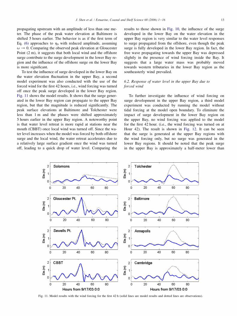
To test the influence of surge developed in the lower Bay onthe water elevation fluctuation in the upper Bay, a secondmodel experiment was also conducted with the use of theforced wind for the first 42 hours, i.e., wind forcing was turnedoff once the peak surge developed in the lower Bay region.Fig. 11 shows the model results. It shows that the surge gener-ated in the lower Bay region can propagate to the upper Bayregion, but that the magnitude is reduced significantly. Thepeak surface elevations at Baltimore and Tolchester wereless than 1 m and the phases were shifted approximately5 hours earlier in the upper Bay region. A noteworthy pointis that water level retreat is more rapid at stations near themouth (CBBT) once local wind was turned off. Since the wa-ter level increases when the model was forced by both offshoresurge and the local wind, the water retreat accelerates due toa relatively large surface gradient once the wind was turnedoff, leading to a quick drop of water level. Comparing the

results to those shown in Fig. 10, the influence of the surgedeveloped in the lower Bay on the water elevation in theupper Bay region is very similar to the water level responsesto surge propagated from the offshore, even though the peaksurge is fully developed in the lower Bay region. In fact, thefree wave propagating towards the upper Bay was depressedslightly in the presence of wind forcing inside the Bay. Itsuggests that a large water mass was probably movedtowards western tributaries in the lower Bay region as thesoutheasterly wind prevailed.

6.2. Response of water level in the upper Bay due toforced wind

To further investigate the influence of wind forcing onsurge development in the upper Bay region, a third modelexperiment was conducted by running the model withouttidal forcing at the model open boundary. To eliminate theimpact of surge development in the lower Bay region onthe upper Bay, no wind forcing was applied to the modelfor the first 42 hour. (i.e., the wind forcing was turned on atHour 42). The result is shown in Fig. 12. It can be seenthat the surge is generated at the upper Bay regions withthe wind forcing only, but no surge was generated in thelower Bay regions. It should be noted that the peak surgein the upper Bay is approximately a half-meter lower than

Fig. 11. Model results with the wind forcing for the first 42 h (solid lines are model results and dotted lines are observations).

14 J. Shen et al. / Estuarine, Coastal and Shelf Science 68 (2006) 1e16

Fig. 12. Model results without tide and with the wind forcing after 42 h (solid lines are model results and dotted lines are observations).

observations at Annapolis and Tolchester, but the peak surgeat Baltimore is very close to observations. The resultindicates the southerly wind is the dominant forcing causingthe high surge in the upper region. The model results showthat there is a set-down in the lower Bay, but it is notsignificant at all. The discrepancy between model resultsand observations can be attributed to the influence of theforerunner caused by the surge that developed in the lowerBay region and propagated northward. Based on the concep-tual model, as shown in Eq. (6) and Fig. 9, we superimposethe surge caused by the local wind and the storm tide gener-ated by storm developed in the offshore and lower Bay re-gions (second run) and display the results in Fig. 13. Theresults show that the superposition of two distinct physical-driven mechanisms agrees quite well with observationdata. It suggests that the storm tide that occurred insidethe Bay during Hurricane Isabel can be well explained bythe conceptual model, which is caused by superposition ofboth remote and local wind effects.

7. Conclusion

The UnTRIM model was used for storm tide simulation inthis study. The model uses an unstructured grid, allowing

boundary fitting and local grid refinements to obtain a finespatial resolution in numerical modeling tasks. The Eulerian-Lagrangian scheme, together with a semi-implicit finite-differ-ence solution method, allows the model to execute with a largeCourant number even though some grid dimensions are lessthan 30 m.

The comparison of harmonic analysis results of tidal simu-lation of the UnTRIM model with those of observations at 11tidal gage stations indicate that the model simulated the char-acteristics of the tidal propagation inside the Bay. The resultsindicate that the model is suitable for long-wave simulation inthe Chesapeake Bay.

The UnTRIM model was applied to simulate HurricaneIsabel in the Chesapeake Bay. The model simulated bothpeak surface elevation and time evolution of the stormtide. The model experiments indicate that water level re-sponse inside the Bay during Isabel can be explained bythe superposition of two distinct physically-driven mecha-nisms: offshore surge propagation into the Bay and localwind. The water level in the lower Bay is more influencedby the offshore condition. The surge developed at theupper Bay is mainly caused by local wind forcing duringHurricane Isabel. The offshore surge propagation into theBay enhanced the surge inside the Bay during HurricaneIsabel.

15J. Shen et al. / Estuarine, Coastal and Shelf Science 68 (2006) 1e16

Acknowledgments

The study is supported by the Southeastern University Re-search Association (SURA). The authors wish to thank Dr. L.Donelson Wright for supporting the model development andDr. Ralph Cheng for many valuable suggestions for the de-velopment of the model. The reviewers’ comments improvedthe manuscript substantially and are kindly appreciated. Thisis Virginia Institute of Marine Science Contribution No.2704.

References

Beven, J., Cobb, H., 2003. Tropical Cyclone Report Hurricane Isabel, National

Hurricane Center. http://www.nhc.noaa.gov/2003isabel.shtml (accessed

date 16.01.04).

Blain, C.A., Westerink, J.J., Luettich, R.A., 1994. The influence of domain

size on the response characteristics of a hurricane storm surge model. Jour-

nal of Geophysical Research 99, 18467e18479.

Fig. 13. Superposition of influences of local wind forcing and offshore surge

(solid lines are model results and dotted lines are observations).

Blumberg, A.F., Mellor, G.L., 1987. A description of a three dimensional

coastal ocean circulation model. In: Heaps, N.S. (Ed.), Three Dimensional

Coastal Ocean Circulation Models, Coastal and Estuarine Sciences 4.

AGU, Washington, DC, pp. 1e16.

Bode, L., Hardy, T.A., 1997. Progress and recent developments in storm surge

modeling. Journal of Hydraulic Engineering 123 (4), 315e331.

Bretschneider, C.L., 1959. Hurricane Surge Predictors for Chesapeake Bay,

US Army Corps of Engineers, Washington, DC, Sept. 1959, Technical Re-

port, AD699408, 51 pp.

Casulli, V., Walters, R.A., 2000. An unstructured grid, three-dimensional

model based on the shallow water equations. International Journal for Nu-

merical Methods in Fluids 32, 331e348.

Casulli, V., June 1999. A semi-implicit numerical method for non-hydrostatic free

surface flows on unstructured grid. Proceedings, International Workshop on

Numerical Modeling of Hydrodynamic Systems, Zaragoza, Spain, 175e193.

Casulli, V., Zanolli, P., 1998. A three-dimensional semi-implicit algorithm for

environmental flows on unstructured grids. In: Proceedings of Conference

on Numerical Methods for Fluid Dynamics. University of Oxford.

Cheng, R.T., Casulli, V., Gartner, J.W., 1993. Tidal, residual, intertidal mudflat

(TRIM) model and its applications to San Francisco Bay, California. Estu-

arine, Coastal, and Shelf Science 36, 235e280.

Cheng, R.T., Casulli, V., 2002. Evaluation of the UnTRIM Model for 3-D

Tidal Circulation, Proceedings of the 7th International Conference,

ASCE, 628e642.

Chuang, W., Boicourt, W., 1989. Resonant seiche motion in the Chesapeake

Bay. Journal of Geophysical Research 94 (C2), 2105e2111.

DeVries, J.W., 1991. The Implementation of the WAQUA/CSM-16 Model for

Real Time Storm Surge Forecasting. KNMI Tech. Rep. TR-131.

Flather, R.A., Proctor, R., Wolf, J., 1991. Oceanographic forecast models.

Computer Modeling in the Environmental Sciences. D.G. Famer and

M.J. Rycroft (Eds.), Oxford. U.K., 15e30.

Garratt, J.R., 1977. Review of drag coefficients over oceans and continents.

Monthly Weather Review 105, 915e929.

Gerritsen, H., de Vries, H., Philippart, M., 1995. The Dutch continental shelf

model. In: Lynch, D.R., Davies, A.M. (Eds.), Quantitative Skill Assess-

ment for Coastal Ocean Models Coastal Estuarine Studies, 47. American

Geophysical Union, Washington, DC, pp. 425e467.

Holland, G.J., 1980. An analytic model of the wind and pressure profiles in

hurricanes. Monthly Weather Review 108, 1212e1218.

Houston, S.H., Shaffer, W.A., Powell, M.D., Chen, J., 1999. Comparison of

HRD and SLOSH surface wind fields in hurricanes: Implications for storm

surge modeling. Weather and Forecasting 14, 671e686.

Hubbert, G.D., McInnes, K.L., 1999. A storm surge inundation model for

coastal planning and impact studies. Journal of Coastal Research 15 (1),

168e185.

Janzen, C.D., Wong, K.-C., 2002. Wind-forced dynamics at the estuary-shelf

interface of a large coastal plain estuary. Journal of Geophysical Research

107 (C10), 3138.

Jelesnianski, C.P., Chen, J., Shaffer, W.A., 1992. SLOSH: sea, lake, and over-

land surges from hurricane. National Weather Service, Silver Springs, MD.

Lippert, C., 2001. Preprocessor JANET, user’s guide. Smile Consult GmbH,

Hanover, 80 pp.

Luettich, R.A., Westerink, J.J., Scheffner, N.W., 1992. ADCIRC: An Advanced

Three-Dimensional Circulation Model for Shelves, Coasts, and Estuaries,

Report I, Theory and Methodology of ADCIRC-2DDI and ADCIRC-

3DL. US Army Corps of Engineers. Technical Report DRP-92e6.

Lynch, D.R., 1983. Progress in hydrodynamic modeling, review of U.S. con-

tributions, 1979e1982. Reviews of Geophysics and Space Physics 21 (30),

741e754.

Mathew, J.P., Mahadevan, R., Bharatkumar, B.H., Subramanian, V., 1996. Nu-

merical simulation of open coast surges. Part I: Experiments on offshore

boundary conditions. Journal of Coastal Research 12, 112e122.

McConochie, J.S., Hardy, T.A., Mason, L.B., 2004. Modelling tropical cyclone

overwater wind and pressure fields. Ocean Engineering 31, 1757e1782.

Mukai, A.Y., Westerink, J.J., Luettich, R.A., 2002. Guidelines for Using East-

coast 2001 Database of Tidal Constituents within Western North Atlantic

Ocean, Gulf of Mexico and Caribbean. US Army Corps of Engineers,

ERDC/CHL CHETN-IV-40, 20 pp.

16 J. Shen et al. / Estuarine, Coastal and Shelf Science 68 (2006) 1e16

Myers, V.A., Malkin, W., 1961. Some properties of hurricane wind fields as

deduced from trajectories. In: National Hurricane Research Project Report,

No. 49. NOAA, U.S. Department of Commerce, 43 pp.

Pore, N.A., 1965. Chesapeake Bay extratropical storm surges. Chesapeake Sci-

ence 6 (3), 172e182.

Powell, M.D., Houston, S.H., Amat, L.R., Morisseau-Leroy, N., 1998. The

HRD real-time hurricane wind analysis system. Journal of Wind Engineer-

ing and Industrial Aerodynamics 77 and 78, 53e64.

Proctor, R., Flather, R.A., 1983. Routine Storm Surge Forecasting using

Numerical Models: Procedure and Computer Programs for use on the

CDC 205E at the British Meteorological Office. Institute of Oceanographic

Sciences. Report No, 167.

Rebay, S., 1993. Efficient unstructured mesh generation by means of Delaunay

triangulation and BowyereWatson algorithm. Journal of Computational

Physics 106, 125e138.

Reid, R.O., 1990. Water level changes. In: Herbich, J. (Ed.), Handbook of

Coastal and Ocean Engineering. Gulf Publishing, Houston, TX.

Scheffner, N., Fitzpatrick, P.L., 1997. Real-time predictions of surge propaga-

tion. In: Spaulding, Malcolm L. (Ed.), Estuarine and Coastal Modeling.

ASCE.

SMS, 2002. Surface water modeling system, tutorials version 8.0, Brigham

Young University e Environmental Modeling Research Laboratory, 216 pp.

Spitz, Y.H., Klinck, J.M., 1998. Estimate of bottom and surface stress

during a spring-neap tide cycle by dynamical assimilation of tide gauge

observations in the Chesapeake Bay. Journal of Geophysical Research

103 (C6), 12761e12782.

Valle-Levinson, A., Wong, K., Bosley, K.T., 2002. Response of the lower

Chesapeake Bay to forcing from hurricane Floyd. Continental Shelf Re-

search 22, 1715e1729.

Verboom, G.K., Ronde, J.G., Van Dijk, R.P., 1992. A fine grid tidal flow and

storm surge model of the North Sea. Continental Shelf Research 12 (2/3),

213e233.

Vested, H.J., Jensen, H.R., Petersen, H.M., 1992. An operational hydrographic

warning system for the North Sea and the Danish Belts. Continental Shelf

Research 12 (1), 65e81.

Wang, D.-P., Elliott, A.J., 1978. Non-tidal variability in the Chesapeake Bay

and Potomac River: evidence for non-local forcing. Journal of Physical

Oceanography 8, 225e232.

Wang, D.-P., 1979a. Subtidal sea level variations in the Chesapeake Bay and rela-

tions to atmospheric forcing. Journal of Physical Oceanography 9, 413e421.

Wang, D.-P., 1979b. Wind-driven circulation in the Chesapeake Bay, winter

1975. Journal of Physical Oceanography 9, 564e572.

Westerink, J.J., Luettich, R.A., Baptista, A.M., Scheffner, N.W., Farrar, P.,

1992. Tide and storm surge predictions using a finite element model.

Journal of Hydraulic Engineering 118, 1373e1390.

Wong, K.-C., Moses-Hall, J.E., 1998. On the relative importance of the remote

and local wind effects to the subtidal variability in a coastal plain estuary.

Journal of Geophysical Research 103 (C9), 18393e18404.