Download pdf - The Application of Committee Machine Model in Power Load Forecasting for the Western Region of Saudi Arabia

JKAU: Eng. Sci., Vol. 22 No.1, pp: 19-38 (2011 A.D. / 1432A.H.)

DOI: 10.4197 / Eng. 22-1.2

19

The Application of Committee Machine Model in Power

Load Forecasting for the Western Region of Saudi Arabia

A.J. Al-Shareef and M.F. Abbod

King Abdulaziz University, Jeddah, Saudi Arabia

School of Engineering and Design, Brunel University, Uxbridge, UK

Abstract. Load forecasting has become in recent years one of the

major areas of research in electrical engineering. Most traditional

forecasting models and artificial intelligence techniques have been

tried out in this task. Artificial neural networks (ANN) have lately

received much attention, and many papers have reported successful

experiments and practical tests. This paper presents the development

of an ANN-based committee machine load forecasting model with

improved accuracy for the Regional Power Control Centre of Saudi

Electricity Company. The proposed system has been further optimized

using Particle Swarm Optimization (PSO) and Bacterial Foraging

(BG) optimization algorithms. Results were compared for standard

ANN, weight optimized ANN, and ANN committee machine models.

The networks were trained with weather-related, time based and

special events indexes for electric load data from the calendar years

2005 to 2007.

Keywords. Artificial neural networks, Short-term load forecasting,

back propagation, Committee machine, Particle swarm

optimization, Bacterial foraging.

List of Symbols

POS : Particle Swarm Optimisation

ANN : Artificial Neural Networks

GB : Bacterial Foraging

STFL: Short Term Load Forecasting

RBF : Radial Basis Functions

MLP: Multi-layer Perceptron


20

1. Introduction

Load forecasting has become in recent years one of the major areas of

research in electrical engineering. Load forecasting is however a difficult

task. First, because the load series is complex and exhibits several levels

of seasonality. Second, the load at a given hour is dependent not only on

the load at the previous day, but also on the load at the same hour on the

previous day and previous week, and because there are many important

exogenous variables that must be considered[1]

. Load forecasting plays an

important role in power system planning and operation. Basic operating

functions such as unit commitment, economic dispatch, fuel scheduling

and unit maintenance, can be performed efficiently with an accurate

forecast[2, 3-4]

.

Various statistical forecasting techniques have been applied to

Short Term Load Forecasting (STLF). Examples of such methods

including, time series[5, 6]

, similar-day approach[7]

, regression methods[5, 8]

and expert systems[7, 9-10]

. In general, these methods are basically linear

models and the load pattern is usually a nonlinear function of the

exogenous variables[1]

. On the other hand, Artificial Neural Networks

(ANN) has been proved as powerful alternative for STLF that does not

rely on human experience. It has been formally demonstrated that ANN’s

are able to approximate numerically any continuous function to the

desired accuracy and it should be expected to model complex nonlinear

relationships much better than the traditional linear models that still form

the core of the forecaster’s methodology. Also, ANN is data-driven

method, in the sense that it is not necessary for the developer to postulate

tentative models and then estimate their parameters. Given a sample of

input and output vectors, ANN is able to automatically map the

relationship[1, 11, 12]

.

This paper presents a study on the use of ANN model to STLF,

particular attention has been given to the network’s topology. Different

techniques were used in the modelling stage, a simple ANN, a weight

optimized ANN, and a committee machine network. Optimization

methods were used to further tune the network for achieving higher

prediction accuracy. The models were developed based on electrical load

data for a typical 24-hours load for the western area of Saudi Arabia.

Time, weather, special season events, and load related inputs are

considered in this model. Three years of historical dependent data were

The Application of Committee Machine Model in Power Load… 21

used. The forecasting system design was customised to features of Saudi

Arabia electrical load.

2. Electric Load Features

Western operational area of Saudi Electricity Company is covering

very important cities with special features. It includes the two holy

mosques in Makkah and Al-Madina, beside, the most economical and

tourism city like Jeddah and other small cities such as Taif and Yanbu.

There are many factors affecting the load of this area, which makes the

forecasting unique and challenging.

The weather changes greatly affecting the load demand due to a

huge air conditioning load in the system. Figure 1 shows a linearity

relationship between system daily peak load and related temperature for

the years 2005-2007. Another important factor is the time of the day, as

social life and activities of the consumers depend on the time of the day

such as working and schools hours and prayer times, as well as the

seasonal load behaviour factor, which reflects how load draws a

changeable profile, due to the impact of seasonality. The effect of

working days and weekends on the load trend is essential. One more

important factor is special events factor mainly religious events such as

the month of Ramadan and Hajj, and other events such as public

holidays, school and exams. These events, based on the lunar calendar

will cause un-similarity in load conditions every year, so that it has to be

considered. Figure 2 shows the electric load data set which is spread over

3 years.

Examples of a daily load consumption profile of a typical

weekday/weekend during summer and winter are shown in Fig. 3. The

difference between winter and summer profiles is clear; the effect of hot

weather is reflected on the great amount of load consumption at

afternoon in the summer day. At Friday a sudden increase in the load

demand afternoon is due to Friday's prayer, and at weekend the load is

stable in the morning.

2.1. Input Vector Indices

The independent variables of the system can be specified as the

date, time, weather conditions, special events data, and associated

historical load data for the day to be forecasted, in hourly bases.


22

Typically, it is configured as seven indexes that represent the time during

the day, date (day, month, year), day type (weekday or weekend),

temperature, relative humidity, wind speed and direction.

2000 3000 4000 5000 6000 7000 800015

20

25

30

35

40

Load (MW)

Tem

pera

ture

(C

)

Fig. 1. Relationship between temperature and the systems daily peak load of 2005.

0 0.5 1 1.5 2 2.5 33000

4000

5000

6000

7000

8000

9000

10000

Load (M

W)

20062005 2007

Fig. 2. Load profile for 3 years.


0 5 10 15 20 252000

3000

4000

5000

6000

7000

8000

9000

10000

Time of the day (hour)

Load (M

W)

Jan/Fri

Jan/Mon

Sept/Fri

Sept/Mon

Fig. 3. Examples of daily load consumption profile of a typical weekday/weekend, winter

and summer days.

Numerical indexes were given to represent the inputs for the

forecasted hour. Indexes of [1:12] were given to represent the month,

[1:24] to represent the hour and [1:7] to represent the day type starting

from Saturday to Friday (the weekend is Thursday and Friday).

Moreover, half-hourly load data is considered for the high load variation

periods of the day, typically 13:30, 14:30, 15:30, 18:30, 19:30 and 20:30

which were represented by the fractions (13.5, 14.5, 15.5, 18.5, 19.5 and

20.5) respectively.

3. Neural Networks Modelling

3.1. Neural Network Training

The ANN models developments were performed using the Matlab

Neural Networks Toolbox. The initial ANN models were trained for the

data using 9 input variables: day, month, year, day type, time of the day,

temperature, humidity, wind speed and wind direction, while the output

is the load. In previous studies [19, 23]

, different ANN topologies were

trained using back propagation training algorithm and tested in order to

find the best network structure that gives the best modelling accuracy.

The ANN topologies were selected as: Linear, Multi-Layer Perceptron

(MLP) and Radial Basis Functions (RBF). A maximum two hidden

layers were selected [14, 16, 17]

. The MLP was found to be the best type of

topology that provides accurate predictions. The data were selected as


24

90% for training (Jan 2005 to September 2007), and 10% for testing

(October – December 2007). Training and testing results are shown in

Fig. 4. Table 1 shows the training results for MLP topology for the

training and testing error. The results are compared to predictions using

logistic regression technique which can show 20.8% improvements in the

testing data prediction accuracy.

0 2000 4000 6000 8000 100000

1000

2000

3000

4000

5000

6000

7000

8000

9000

10000training

actual load

pre

dic

ted load

(a) Training

0 2000 4000 6000 8000 100000

1000

2000

3000

4000

5000

6000

7000

8000

9000

10000testing

actual load

pre

dic

ted load

(b) Testing

Fig. 4. Simple ANN training and Testing (single layer, 18 hidden neurons, 100 epochs).


Table 1. ANN training and testing RMS results.

Training Testing Testing Improvements

(%)

Logistic Regression 25.4507 25.0036 -

Standard ANN 19.3296 19.8466 20.8

3.2. ANN Weights Optimization

For the MLP topology of 1 hidden layer with 18 hidden neurons, 9

inputs and a single output, there are 166 parameters in the network that are

adjusted and optimized during the learning phase. However, due to the

learning algorithm shortcoming, sometime the back propagation learning

algorithm falls short of finding the exact parameters for the optimum solution.

Therefore, an optimization algorithm can improve the prediction accuracy by

fine tuning the ANN parameters within a constrained range. In this stage, two

optimization algorithms were utilized, namely Particle Swarm Optimization

and Bacterial Foraging, in order to fine tune the weights in the network with a

margin of 10% change for each parameter.

3.2.1. Particle Swarm Optimization Algorithm (PSO)

Particle Swarm Optimization is a global minimization technique [24, 25]

for dealing with problems in which a best solution can be represented as

a point or and a velocity. Each particle assigns a value to the position

they have, based on certain metrics. They remember the best position

they have seen, and communicate this position to the other members of

the swarm. The particles will adjust their own positions and velocity

based on this information. The communication can be common to the

whole swarm, or be divided into local neighbourhoods of particles.

With the PSO algorithm constant weights factors 9c1 and c2) were

set to c1 = 1.49618; c2 = 1.49618; while the inertia weight (w) was set to

w = 0.7298. The algorithm was set to start with a random weights tuning

which has recorded an increment in the training data RMS. The PSO

algorithm was iterated for 100 epochs which has achieved a smaller

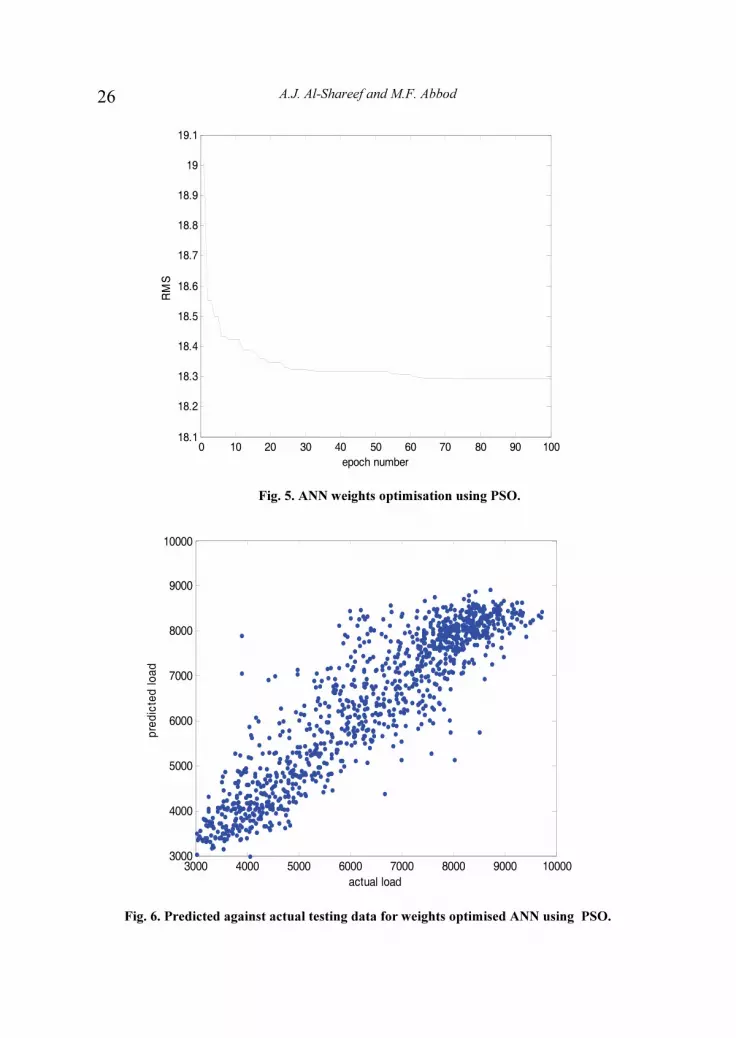
RMS. Figure 5 shows the training RMS error against the iteration

number. The tuned network was tested using the testing data and the

recorded RMS has also shown an improvement compared to the standard

ANN. Figure 6 shows the optimized ANN prediction against the actual

loads for the testing data.


26

0 10 20 30 40 50 60 70 80 90 10018.1

18.2

18.3

18.4

18.5

18.6

18.7

18.8

18.9

19

19.1

epoch number

RMS

Fig. 5. ANN weights optimisation using PSO.

Fig. 6. Predicted against actual testing data for weights optimised ANN using PSO.

3000 4000 5000 6000 7000 8000 9000 100003000

4000

5000

6000

7000

8000

9000

10000

pre

dic

ted

lo

ad

actual load


3.2.2. Bacterial Foraging Optimization Algorithm (BG)

Recently, search and optimal foraging of bacteria have been used

for solving optimization problems [21, 26]

. To perform social foraging, an

animal needs communication capabilities and over a period of time it

gains advantages that can exploit the sensing capabilities of the group.

This helps the group to predate on a larger prey, or alternatively,

individuals could obtain better protection from predators while in a

group.

Its behaviour and movement comes from a set of six rigid spinning

(100–200 r.p.s) flagella, each driven as a biological motor. An E. coli

bacterium alternates through running and tumbling. Running speed is 10–

20 lm/s, but they cannot swim straight. The chemotactic actions of the

bacteria are modelled as follows:

• In a neutral medium, if the bacterium alternatively tumbles and

runs, its action could be similar to search.

• If swimming up a nutrient gradient (or out of noxious substances)

or if the bacterium swims longer (climb up nutrient gradient or down

noxious gradient), its behaviour seeks increasingly favourable

environments.

• If swimming down a nutrient gradient (or up noxious substance

gradient), then search action is like avoiding unfavourable environments.

Therefore, it follows that the bacterium can climb up nutrient hills

and at the same time avoids noxious substances. The sensors it needs for

optimal resolution are receptor proteins which are very sensitive and

possess high gain. That is, a small change in the concentration of

nutrients can cause a significant change in behaviour. This is probably

the best-understood sensory and decision-making system in biology [21]

.

At this stage, the BG optimization algorithm was utilized to fine

tune the NN weights in a similar fashion to the PSO algorithm. Figure 7

shows the training RMS for the same number of iterations. Figure 8

shows the optimized ANN prediction against the actual loads for the

testing data.


28

Fig. 7. ANN weights optimization using BG.

Fig. 8. Predicted against actual testing data for weights optimized ANN using BG.

Table 2 shows a comparison between the two optimization

algorithms for the training and testing errors. Both algorithms show

improvements in the testing data prediction accuracy. However the PSO

3000 4000 5000 6000 7000 8000 9000 100003000

4000

5000

6000

7000

8000

9000

10000

actual load

pre

dic

ted load

0 10 20 30 40 50 60 70 80 90 100

18

20

22

24

26

28

30

32

34

36

38

RMS

iteration number


has achieved 26.8% improved prediction compared to the BG algorithm

which has achieved 25.6%. There is a 5% improvement in the

performance compared to standard ANN.

Table 2. ANN training and testing RMS using PSO and BG weights optimization.

Training Testing

Testing

Improvements (%)

PSO 18.2908 18.3856 26.8

BG 18.5544 18.6378 25.6

3.3. Committee Machine

Ensembles are a well established method for obtaining highly

accurate classifiers by combining different algorithms. A number of

researchers have applied ensemble methods to improve the performance

of neural networks [22, 27]

. The basic idea of a committee machine is to

combine a mixture of experts and to effectively make use of the results

produced by each expert within the ensemble. Figure 9 provides the

architecture of the committee machine system with 10 copies of the same

algorithm. By combining the result of each classifier, the final result can

be realized with improved performance. Each classifier gives its result R

and the confidence Cf for the result to the combiner. The confidence is

utilised as a weighted vote for the combiner to avoid affecting the final

decision by the result of individual expert featuring low confidence.

The committee machine modelling approach used in this paper

consists of two stages: generating of individual candidate neural

networks while the second stage is combining the individual neural

networks into an ensemble model. In the first stage, it is necessary to

determine what variations, such as the initial weights, training algorithms

and training options, training data etc., are to be introduced to generate

the individual models. Standard training procedure can then be used to

generate the models. Some discretion needs to be applied during the

training of the individual models, since in some cases training might end

up with a poor model and it is not wise to include such a poor model into

the ensemble candidates. The aim of the first stage is to produce an

ensembled neural network models with acceptable prediction

performance, and confidence bands.

The ensemble model has many advantages over its single (best)

neural network model; among these are the improvement of prediction

accuracy, the strong robustness, and better generalization ability.


30

Moreover, it can give an error bound on its prediction as a by-product,

since all the individual models in the ensemble set are different and the

difference in their predictions can be used as an indication of the

reliability of the ensemble model on the given input. Based on this

concept, the error bound can be calculated from the standard deviation of

the individual predictions. For a given prediction )(ˆ ky , its error is given

by:

∑∑==

=−==

N

i

i

N

i

iky

Nkykyky

NkkEB

11

2 )(1

)(ˆ;))(ˆ)((1

2)(2)( σ (1)

where )(ˆ ky is the output of the ensemble model for input x(k), yi(k) is the

corresponding output of the i th neural network, EB(k) is the error bounds

for the )(ˆ ky with 95% confidence, N is the number of neural networks in

the ensemble set, and σ(k) is the standard deviation among the output

predictions yi(k). Apparently, the error bounds will be affected by the

characteristics of input regions where prediction is to be made. Generally

speaking, the error bound tends to be small in regions covered by dense

training data, and vice versa.

Fig. 9. Ensembled NN embedded in the committee machine architecture.

In the second stage the individual ensemble neural networks are

combined into the committee machine. Using the confidence band as a

weight coefficient for each classifier will therefore give very little

weighting coefficient to the best classifier over the worst one. In this

work, an optimization method is proposed to tune the weighting factor of

each member on the machine. The weighting function defined by:

Wi = Pi Pw Pop (2)

ENN1

ENN2

Combine

ENNn

Results and

confidence

Input data Prediction

.

.


where Wi is the weight of a given predictor i with a given prediction Pi.

Pi is defined as the average prediction performance of each individual

ensembled NN models in the committee machine. Pop is the optimiser

weighing which can be adjusted during the optimization process. Pw is

the predictor confidence based on its prediction performance within the

ensemble.

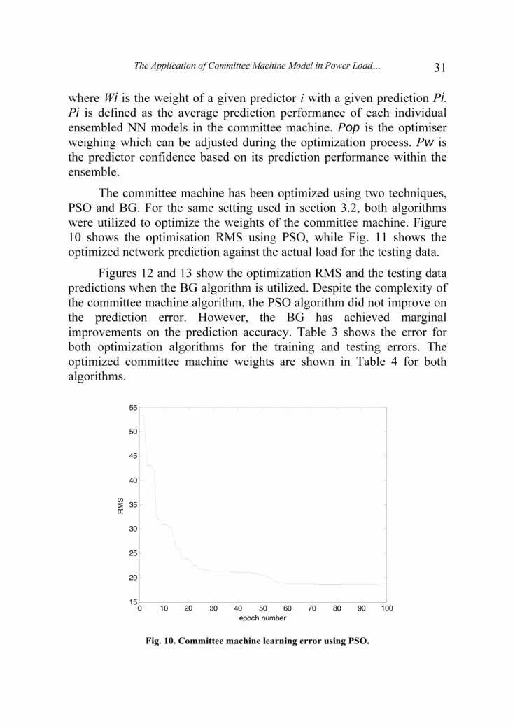
The committee machine has been optimized using two techniques,

PSO and BG. For the same setting used in section 3.2, both algorithms

were utilized to optimize the weights of the committee machine. Figure

10 shows the optimisation RMS using PSO, while Fig. 11 shows the

optimized network prediction against the actual load for the testing data.

Figures 12 and 13 show the optimization RMS and the testing data

predictions when the BG algorithm is utilized. Despite the complexity of

the committee machine algorithm, the PSO algorithm did not improve on

the prediction error. However, the BG has achieved marginal

improvements on the prediction accuracy. Table 3 shows the error for

both optimization algorithms for the training and testing errors. The

optimized committee machine weights are shown in Table 4 for both

algorithms.

0 10 20 30 40 50 60 70 80 90 10015

20

25

30

35

40

45

50

55

epoch number

RMS

Fig. 10. Committee machine learning error using PSO.


32

3000 4000 5000 6000 7000 8000 9000 100003000

4000

5000

6000

7000

8000

9000

10000

actual load

pre

dic

ted load

Fig. 11. NN committee machine predicted against actual load for testing data.

0 10 20 30 40 50 60 70 8010

15

20

25

30

35

40

45

50

ittiration number

RMS

Fig. 12. Committee machine learning error using BG.


3000 4000 5000 6000 7000 8000 9000 100003000

4000

5000

6000

7000

8000

9000

10000

actual load

pre

dic

ted load

Fig. 13. BG committee machine testing data predictions.

Table 3. NN training and testing RMS using PSO and BG.

Training Testing Testing Improvements (%)

PSO 18.4800 18.4792 26

BG 14.5750 14.6788 41.6

Table 4. Ensembled weights optimization using PSO and BG.

NN1 NN2 NN3 NN4 NN5 NN6 NN7 NN8 NN9 NN10

PSO 0.5721 1.0005 0.6946 1.2257 1.0390 1.0483 0.9602 1.0162 0.8896 1.0788

BG 1.0031 1.0524 0.9478 0.9605 0.9517 0.9034 1.0440 0.9906 1.0861 0.9162

Despite the fact that both PSO and BG have shown equivalent

improvements when used to optimize the ANN, the use of BG with the

committee machine algorithm proves the BG can perform better results

for a complex system. The improvements have been raised to 40% which

proves that PSO can handle simple system only due to its algorithm

simplicity, whereas BG is more complicated and can achieve better

results.


34

4. Conclusion

This paper presents an ANN system for predicting the electrical

loads on the Western grid in the Kingdom of Saudi Arabia. This network

has a load pattern with special features. These features are to cope with

the special religious activities. Moreover, the load pattern is much

affected by the time schedule, the temperature, humidity, wind speed and

direction. The load patterns have varying features especially in the holy

cities of Makkah and Madinah which host millions of people in different

seasons during the year to perform religious activities. In fact, the

religious tourism influences the system load profile [19]

. Different

modelling techniques were used, a standard MLP ANN was utilised to

develop a standard model, and consequently optimized further using PSO

and BG. The advantages of the ANN is that it can cope with large

number of data and high input dimension, this is a positive feature with

load data, as it has high dimension and vast amount of data point.

However, due to the noise in the data and the variation of the load, the

ANN training algorithm does not guarantee a optimum network which is

a disadvantage of the algorithm. An assistant tool need to be introduced

to the system so that the network can learn the least error. This can be

achieved by the introduction of an optimization algorithm or an

ensemble. A more sophisticated algorithm was also investigated which is

based on committee machine. Committee machine has the advantage of

combining many ANN together so that the network which has some

misfit in a specific area of the model can be compensated by the other

networks. However, the committee machine algorithm will require

further tuning in order to find the weights of each network. The algorithm

was further optimized using PSO and GB. Improved results have been

achieved using the committee machine modelling technique. The two

optimization algorithms are simple and fast in finding the optimal setting

of the algorithm, PSO in particular has a simple structure but it can only

do search locally, on the other hand, BG is better searching algorithm but

it is more sophisticated which consequently takes longer calculation time.

Acknowledgments

This research is conducted with support from the KSACT, Saudi

Arabia. The authors also would like to thank SEC-WOA Company,

System Operations and Control Department-West, for providing the

electrical load and weather data used in this research.


References

[1] Hippert, H. S., Pedreira, C. E. and Souza, R. C., “Neural networks for short-term load

forecasting: A review and evaluation,” IEEE Trans. Power Syst., 16(1):44-55(Feb. 2001).

[2] Alsayegh, O. A., “Short-term load forecasting using seasonal artificial neural networks,”

International Journal of Power and Energy Systems, 23 (3):137-142(2003).

[3] Senjyu, T., Takara, H., Uezato, K. and Funabashi, T., “One hour-ahead load forecasting

using neural network,” IEEE Trans. Power Systems, 17(1) : 113-118 (Feb. 2002).

[4] Baklrtzis, A. G., Petrldis, V., Klartzis, S. J., Alexiadls, M. C. and Malssis, A .H., “A

neural network short term load forecasting model for the Greek power system,” IEEE Trans.

Power Systems, 11(2):858-863, May(1996).

[5] Tripathi, M.M., Upadhyay, K.G. and Singh, S.N., “Short-Term Load Forecasting Using

Generalized Regression and Probabilistic Neural Networks in the Electricity Market,” The

Electricity Journal, 21(9):24-34 (2008).

[6] Taylor, J.W., de Menezes, L.M. and McSharry, P.E., “A comparison of univariate

methods for forecasting electricity demand up to a day ahead, ” International Journal of

Forecasting, 22: 1-6 (2006).

[7] Drezga, I. and Rahman, S., “Short-term load forecasting with local ANN predictors,” IEEE

Trans. Power Systems, 14(3): 844–850, Aug (1999).

[8] Zivanovic, R., “Local regression-based-short term load forecasting,” Journal of Intelligent &

Robotic Systems, 31(1-3) : 115-127 (2001).

[9] Rahman S. and Hazim, O., “A generalized knowledge-based short term load forecasting

technique”, IEEE Trans. Power Systems, 8(2): 508-514, May (1993).

[10] Kodogiannis, V.S. and Anagnostakis, E.M., “Soft computing based techniques for short-

term load forecasting,” Fuzzy Sets and Systems, 128(3): 413-426 (2002).

[11] H. Chen, C.A. Canizares, and A. Singh. “ANN-based short-term load forecasting in

electricity markets,” Proceedings of the IEEE Power Engineering Society Transmission and

Distribution Conference, 2:411 415, 2001.

[12] Taylor J.W. and Buizza, R., “Neural Network Load Forecasting with Weather Ensemble

Predictions”, IEEE Trans. Power Systems, 17: 626-632, (2002).

[13] Hagan, M. T., Demuth, H. B. and Beale, M.H., “Neural Networks Design,” Boston, MA:

PWS Publishing (1996).

[14] Haykin, S., “Neural Network- a Comprehensive Foundation,” Prentice Hall International,

Second edition (1998).

[15] Senjyu, T., Mandal, P., Uezato, K. and Funabashi, T., “Next Day Load Curve Forecasting

Using Hybrid Correction Method”, IEEE Trans. Power Systems, 20(1) Feb (2005).

[16] MacKay, D. J. C., “Bayesian interpolation”, Neural Computation, 4: 415-447 (1992).

[17] Foresee, D. and Hagan, F., “Gauss-Newton approximation to Bayesian learning,”

International Conference on Neural Networks, 3: 1930-1935(1997).

[18] Hunter, C.M., Moller, H. and Fletcher, D., “Parameter uncertainty and elasticity analyses

of a population model: setting research priorities for Shearwaters,” Ecol. Model., 134:299–

324 (2000).

[19] Al-Shareef, A. J., Mohamed, E. A. and Al-Judaibi, E., “One Hour Ahead Load Forecasting

Using Artificial Neural Network for the Western Area of Saudi Arabia,” International

Journal of Electrical Systems Science and Engineering, 1(1): 35-40(2008).

[20] Kennedy, J. and Eberhart, R., “Particle Swarm Optimization”, Proc. IEEE Int'l. Conf. on

Neural Networks, Perth, Australia, November (1995), pp: 1942-1948.

[21] Gazi, V. and Passino, K.M., Stability analysis of social foraging swarms, IEEE Transactions

on Systems Man and Cybernetics Part B – Cybernetics, 34 (1): 539–557 (2004).

[22] Su, M. and Basu, M. “Gating Improves Neural Network Performance,” Proc. IEEE Conf.

IJCNN, (2001), vol. 3, pp. 2159–2164.


36

[23] Alshareef, A.J., Mohammed, E.A. and Aljoudabi, E.,"Next 24 hour Load Forecasting

Using Artificial Neural Network for the Western Region", JKAU:Eng.Sci, 19(2): 25-40

(2008).

[24] Kennedy, J. and Eberhart, R., “Particle swarm optimization”, Proc. of the IEEE Int. Conf.

on Neural Networks, Piscataway, NJ, (1995), pp: 1942–1948.

[25] Kennedy, J. and Eberhart, R.C., "Swarm Intelligence", Morgan Kaufmann (2001). ISBN 1-

55860-595-9.

[26] Gazi, V. and Passino, K.M., "Stability Analysis of Social Foraging Swarms", IEEE

Transactions on Systems Man and Cybernetics Part B – Cybernetics, 34(1): 539–557(2004).

[27] Shi, M., Bermak, A., Belhouari, S.B. and Chan, C.H., "Gas Identification Based on

Committee Machine for Microelectronic Gas Sensor", IEEE Transactions on Instrumentation

and Measurements, 55(5):1786-1793(2006).


Appendix

Correlation Analysis

The correlation is one of the most common and useful statistical analysis tools that can be

used in data modelling and analysis. A correlation is a number that describes the degree of

relationship between two variables. The correlation is defined as the covariance between Xi and

Xj divided by the product of their standard deviations. Matlab provides a function for calculating

the correlation matrix of a set data with multiple variables. A correlation study has been

conducted to test the relationship between the input variables and the load. The aim of this test is

to see how much each variable is related to the load forecasting, so the variable can either be

considered as important or redundant that can be dropped from the data set for the purpose of

simplifying the developed models. Table A1 shows the correlation matrix. An extra input variable

has been added to the data set as the day number in the week (Sat:1 – Fri:7). The correlation

matrix shows that the month, year, time and day type variables have considerable correlation to

the output, while the temperature, wind direction and humidity have significant correlation with

the load. Otherwise, the other variables, day and day type have low correlation.

Table A1. Correlation table of the load with respect to the individual input variables.

Input variables Load Rank

Day -0.0007 9

Month 0.3334 2 Date

Year 0.1731 4

Event Day type -0.0287 8

Time Hours 0.0795 7

Temperature 0.5775 1

Humidity 0.1020 5

Wind speed -0.0964 6

Atmosphere

Wind direction 0.2856 3


38

��

� �� !�� "��– ��

��#��

��

��

��

�� . ��

�� ! ��

"�#�� $% �� &��'�� ()*�� +��*�� ,�'. ��-��

/(& ��* �� -� 0�1�� 2��*%� /(& �3�� &��'��

�� +��*�� *�)��'* ��&��'�� -�� 4��

�� 5 �� . 6$ �� '* �5� �� 7$% 0�8**

�& �� 9*�� 0��&��'�� -( :��*� /(& � ��(�

�8�� #�� )'�� 2��*�� 3�� +��*��

;��(� �� 9�� -�� . 2�<� =� >�� 2* 4�*)�� 6$ ��

:��*� /(& � ��(� ?��*�� -*�� 3�(� �1�� -��

�� )� 21 �� *�� 2*>��@ 4�*)�� 6$ �� A :��*� 0�

��-(� /(1�� 0�3 � ��&��'�� 9�� -�� =� .

��#*� =� ��* 2* ��#�� )'�� -

�� 0��3�� B)'��):�� –0�8�� D��9�� ( /�@ ��8@

0� ��*F�� 0�� 2�5GHHIDم ٢٠٠٧.