1

Time synchronization in

Wireless Sensor Networks

Smart Sensors and Sensor Networks

Ariana BITU MIT I

Timisoara 2014

2

Table of Contents

1. Introduction

1.1 The approached domain................................................................................................3

1.2 General Information about sensor networks.................................................................3

1.3 General Information about time synchronization in WSNs..........................................4

1.4 Synchronization issues …………………………………………………………..…….5

2 Synchronization protocols……………………………………………………………...6

3 Gradient Time Synchronization Protocol (GTSP) …………………………………...7

3.1 Hardware and Logical clock…………………………………………………………….8

3.2 Synchronization algorithm ……………………………………………………………..9

3.2.1 Drift compensation…………………………………………………………...10

3.2.2 Offset compensation………………………………………………………….11

3.2.3 Computation and memory requirements……………………………………..12

3.2.4 Energy efficiency……………………………………………………………..12

3.3 Target platform used for implementation……………………………………....12

3.4 MAC Layer Timestamping…………………………………………………….14

3.5 Evaluating performances……………………………………………………….16

3. Conclusions……………………………………………………………………….…….18

4. References………………………………………………………………………………19

3

INTRODUCTION

1.1 The approached domain Time is one of the most important factors in a WSN, because the accuracy of time gives the precision of the information for basic communication, but it also provides the ability to detect movement, location, and proximity, if the time is not accurate the information provided is not reliable. It is desired that the collected information is accompanied by additional time data that would provide knowledge about when that information was collected. To obtain the reliability of the information provided the time should be the same in all of the sensors of a network. Time synchronization is important because it can be used in different forms by the protocols that ensure data communication between sensors.

1.2 General Information about wireless sensor network

The WSN’s are built of "nodes" that range from a few to several hundreds or even thousands,

where each node is connected to one (or sometimes several) sensors. Every sensor has three

basic units- sensing, radio, and battery, the major constraint being limited energy as the sensor

nodes are directly dependent on the battery life[1]. Sensor networks are composed of small,

battery operated sensors, whose main function is to collect and forward the required data to the

base stations.

The development of wireless sensor networks was motivated by military applications such as

battlefield surveillance; today such networks are used in many industrial and consumer

applications, such as industrial process monitoring and control, machine health monitoring, and

so on.

Wireless sensor networks have been successfully applied in various application domains such as:

Air quality monitoring:

The most important applications relates for real time monitoring of quality of the air or

monitoring dangerous gases is particularly interesting in hazardous areas because it can have

a bad consequences.

Forest fire detection

A network of Sensor Nodes can be installed in a forest to detect when a fire has started. They

are very useful because it can detect fire before it too late

Smart home monitoring

The activities performed in a smart home can watched anytime do you want to know whether

is in safe anytime when you`re gone.

Military

Detection of nuclear, biological, and chemical attacks and presence of hazardous materials.

Prevention of enemy attacks via alerts when enemy aircrafts are spotted. Monitoring friendly

forces, equipment and ammunition.

4

1.3 General Information about time synchronization in WSNs

Time synchronization in all networks either wired or wireless is important. It allows for

successful communication between nodes on the network. It is, however, particularly vital for

wireless networks. Synchronization in wireless nodes allows for a TDMA algorithm to be

utilized over a multi-hop wireless network[2].

TDMA (Time division multiple access) – a reliable protocol developed and owned by Intel

specifically for improving the performance of long distance links. The protocol allows several

users to share the same frequency channel by dividing the signal into different time slots. The

users transmit in rapid succession, one after the other, each using its own time slot. This allows

multiple stations to share the same transmission medium while using only a part of its channel

capacity. When the channel is not used, it can be turned off, for power saving reasons.

In distributed systems, there is no global clock or common memory. Each processor has its own internal clock and its own notion of time. In practice, these clocks can easily drift seconds per day, accumulating significant errors over time. Also, because different clocks tick at different rates, they may not remain always synchronized although they might be synchronized when they start. This clearly poses serious problems to applications that depend on a synchronized notion of time. The usage of the internal clock of a sensor would not be a good solution, because if each sensor uses its own internal clock no synchronization will be done between them. Even if the initial configuration is well done, the differences that will appear between them will increase by time. To prevent this some kind of information exchange must be done across the network and the sensors should adjust their internal clock from time to time.

In sensor networks when the nodes are deployed, their exact location is not known so time synchronization is used to determine their location. Also time stamped messages will be transmitted among the nodes in order to determine their relative proximity to one another. Time synchronization is used to save energy; it will allow the nodes to sleep for a given time and then awaken periodically to receive a beacon signal. Many wireless nodes are battery powered, so energy efficient protocols are necessary. Lastly, having common timing between nodes will allow for the determination of the speed of a moving node[2]. The need for multi-hop communication arises due to the increase in the size of wireless sensor networks. In such settings, sensors in one domain communicate with sensors in another domain via an intermediate sensor that can relate to both domains. Communication can also occur as a sequence of hops through a chain of pairwise-adjacent sensors. The clock synchronization for multi-hop communication needs to be done in such a way that the skew between different nodes of the network should be reduced to minimum, without taking into account the distance between them. This fact is known as global clock skew minimization. In the same time the clock synchronization between nodes that are closer one to

5

each other is also important. For example let us suppose that we want to receive an acoustic signal that would processed further. All the nodes that will receive that signal must be well synchronized so that the localization of the signal would have higher accuracy. In Media Access Control layer the most important thing is that the nodes should prevent transmission collisions so that the message transmission between one sender and the intended receiver node(s) does not interfere with transmission by other nodes. In this case the focus in on the local clock skew minimization, because the collisions could appear between closer nodes and not between far nodes.

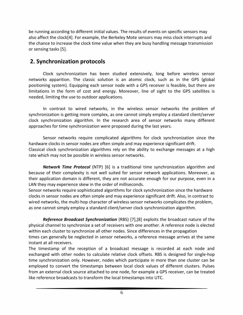
1.4 Synchronization issues Wireless sensor networks provide answers to user queries by fusing data from each sensor to form a single answer or result. To accomplish this data fusion, it becomes necessary for these sensors to agree on a common notion of time. All the participating sensors can be enveloped in a common time scale by either synchronizing the local clocks in each sensor or by just translating timestamps that arrive at a sensor into the local clock times[3]. The time of a computer clock is measured as a function of the hardware oscillator

(1)

Where is the angular frequency of the oscillator, k is a constant for that oscillator, and t

is the time. The change of the value leads to the events (or interrupts) that can be captured by the sensor. The clocks in a sensor network can be inconsistent due to several reasons. The clock may drift due to environment changes, such as temperature, pressure, battery voltage, etc. There are three reasons for the nodes to be representing different times in their respective clocks:

The nodes might have been started at different times

The quartz crystals at each of these nodes might be running at slightly different frequencies, causing the clock values to gradually diverge from each other (termed as the skew error)

The frequency of the clocks can change variably over time because of aging or ambient conditions such as temperature (termed as the drift error)[4].

All the above said errors are three sources that contribute to different time within a sensor network. The nodes in a sensor network may not be synchronized well initially, when the network is deployed. The sensors may be turned on at the different times and their clocks may

6

be running according to different initial values. The results of events on specific sensors may also affect the clock[4]. For example, the Berkeley Mote sensors may miss clock interrupts and the chance to increase the clock time value when they are busy handling message transmission or sensing tasks [5].

2. Synchronization protocols

Clock synchronization has been studied extensively, long before wireless sensor networks apparition. The classic solution is an atomic clock, such as in the GPS (global positioning system). Equipping each sensor node with a GPS receiver is feasible, but there are limitations in the form of cost and energy. Moreover, line of sight to the GPS satellites is needed, limiting the use to outdoor applications.

In contrast to wired networks, in the wireless sensor networks the problem of synchronization is getting more complex, as one cannot simply employ a standard client/server clock synchronization algorithm. In the research area of sensor networks many different approaches for time synchronization were proposed during the last years.

Sensor networks require complicated algorithms for clock synchronization since the hardware clocks in sensor nodes are often simple and may experience significant drift. Classical clock synchronization algorithms rely on the ability to exchange messages at a high rate which may not be possible in wireless sensor networks.

Network Time Protocol (NTP) [6] is a traditional time synchronization algorithm and because of their complexity is not well suited for sensor network applications. Moreover, as their application domain is different, they are not accurate enough for our purpose, even in a LAN they may experience skew in the order of milliseconds. Sensor networks require sophisticated algorithms for clock synchronization since the hardware clocks in sensor nodes are often simple and may experience significant drift. Also, in contrast to wired networks, the multi-hop character of wireless sensor networks complicates the problem, as one cannot simply employ a standard client/server clock synchronization algorithm.

Reference Broadcast Synchronization (RBS) [7],[8] exploits the broadcast nature of the physical channel to synchronize a set of receivers with one another. A reference node is elected within each cluster to synchronize all other nodes. Since differences in the propagation times can generally be neglected in sensor networks, a reference message arrives at the same instant at all receivers. The timestamp of the reception of a broadcast message is recorded at each node and exchanged with other nodes to calculate relative clock offsets. RBS is designed for single-hop time synchronization only. However, nodes which participate in more than one cluster can be employed to convert the timestamps between local clock values of different clusters. Pulses from an external clock source attached to one node, for example a GPS receiver, can be treated like reference broadcasts to transform the local timestamps into UTC.

7

The Routing Integrated Time Synchronization protocol (RITS) [9] provides post-facto synchronization. Detected events are time-stamped with the local time and reported to the sink. When such an event timestamp is forwarded towards the sink node, it is converted from the local time of the sender to the receiver’s local time at each hop. A skew compensation strategy improves the accuracy of this approach in larger networks.

The Timing-sync Protocol for Sensor Networks (TPSN) [10 ]propose to provide network-wide time synchronization. The TPSN algorithm elects a root node and builds a spanning tree of the network during the initial level discovery phase. In the synchronization phase of the algorithm, nodes synchronize to their parent in the tree by a two-way message exchange. Using the timestamps embedded in the synchronization messages, the child node is able to calculate the transmission delay and the relative clock offset. Timing-sync Protocol for Sensor Networks does not compensate for clock drift which makes frequent resynchronization mandatory. In addition, TPSN causes a high communication overhead since a two-way message exchange is required for each child node.

Flooding-Time Synchronization Protocol (FTSP) [11] solve the problem from TPSN. A root node is elected which periodically floods its current timestamp into the network forming an ad-hoc tree structure. MAC layer time-stamping reduces possible sources of uncertainty in the message delay. Each node uses a linear regression table to convert between the local hardware clock and the clock of the reference node. The root node is dynamically elected by the network based on the smallest node identifier. After initialization, a node waits for a few rounds and listens for synchronization beacons from other nodes. Each node sufficiently synchronized to the root node starts broadcasting its estimation of the global clock. If a node does not receive synchronization messages during a certain period, it will declare itself the new root node.

The Reachback Firefly Algorithm (RFA) [12] is inspired from the way neurons and fireflies spontaneously synchronize. Each node periodically generates a message and observes messages from other nodes to adjust its own firing phase. RFA only provides synchronicity, nodes agree on the firing phases but do not have a common notion of time. Another shortcoming of RFA is the fact that it has a high communication overhead. The fundamental problem of clock synchronization has been studied extensively and many theoretical results have been published which give bounds for the clock skew and communication costs.

Srikanthand Toueg [13] presented a clock synchronization algorithm which minimizes

the global skew, given the hardware clock drift.

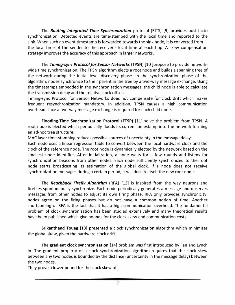
The gradient clock synchronization [14] problem was first introduced by Fan and Lynch in. The gradient property of a clock synchronization algorithm requires that the clock skew between any two nodes is bounded by the distance (uncertainty in the message delay) between the two nodes. They prove a lower bound for the clock skew of

8

(2) for two nodes with distance d, where D is the network diameter. This lower bound also holds if delay uncertainties are neglected and an adversary can decide when a sync message will be sent.

The Time-Diffusion Protocol (TDP) [15] by Su and Akyildiz achieves a network-wide “equilibrium” time usingan iterative, weighted averaging technique based on a diffusion of messages involving all the nodes in the synchronization process.

The Asynchronous Diffusion Protocol [16] by Li and Rus uses a strategy similar to TDP; however, network nodes execute the protocol and correct their clocks asynchronously with respect to each other.

3. Gradient Time Synchronization Protocol (GTSP)

In the article named Gradient Clock Synchronization in Wireless Sensor Networks written by Philipp Sommer and Roger Wattenhofer [17], the autors are proposing the Gradient Time Synchronization Protocol (GTSP) as a method of clock synchronization and they demonstrate how this method can be used for a better synchronization of close-by nodes in a network. The Gradient Time Synchronization Protocol (GTSP) is designed to provide accurately synchronized clocks between neighbors. GTSP works in a completely decentralized fashion: Every node periodically broadcasts its time information. Synchronization messages received from direct neighbors are used to calibrate the logical clock. The basic idea of the algorithm is to provide precise clock synchronization between direct neighbors while each node can be more loosely synchronized with nodes more hops away. The model proposed in [17] assume that the number of nodes are equipped with a hardware clock subject to clock drift. Furthermore, nodes can convert the current hardware clock reading into a logical clock value and vice versa.

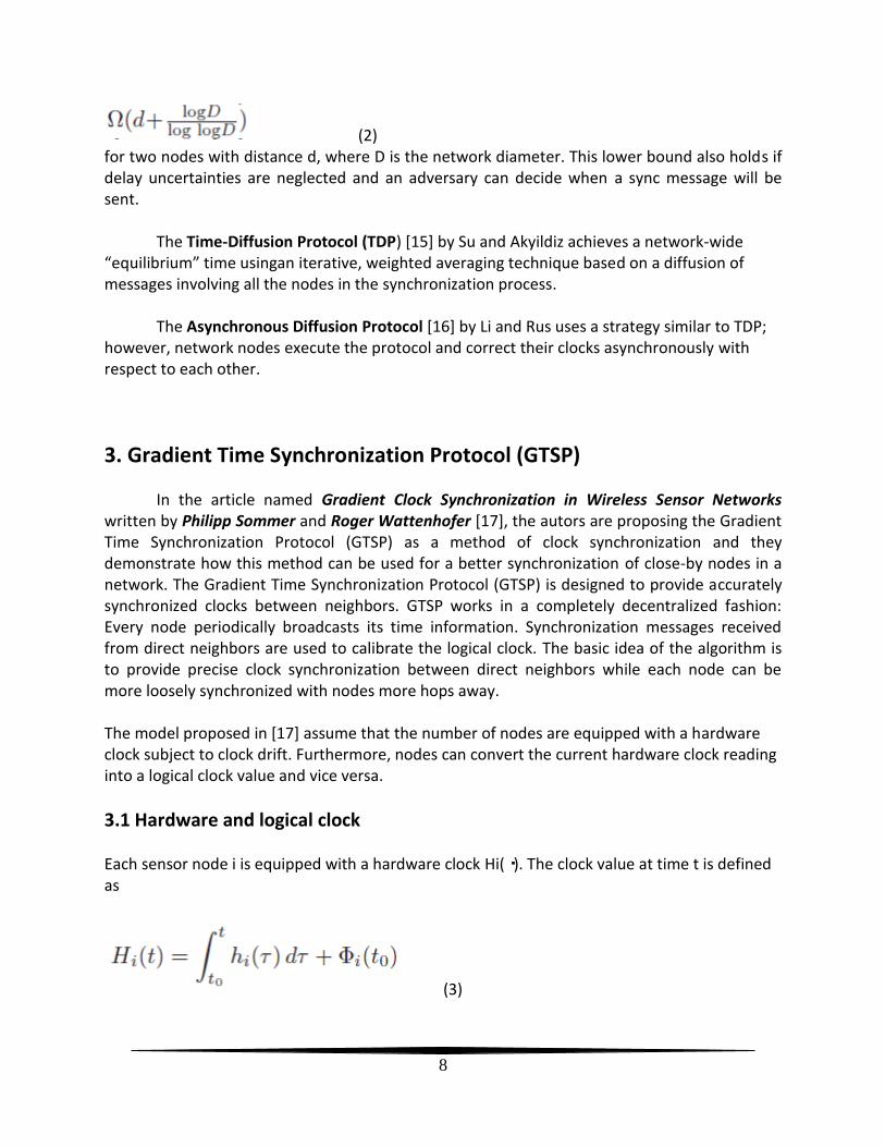
3.1 Hardware and logical clock Each sensor node i is equipped with a hardware clock Hi(・). The clock value at time t is defined as

(3)

9

where hi(τ ) is the hardware clock rate at time τ and Φi(t0) is the hardware clock offset at time t0. It is assumed that hardware clocks have bounded drift, i.e., there exists a constant 0 ≤ ρ < 1 such that

(4) for all times t. This implies that the hardware clock never stops and always makes progress with at least a rate of 1 − ρ. This is a reasonable assumption since common sensor nodes are equipped with external crystal oscillators which are used as clock source for a counter register of the microcontroller. These oscillators exhibit drift which is only gradually changing depending on the environmental conditions such as ambient temperature or battery voltage and on oscillator aging. This allows to assume the oscillator drift to be relatively constant over short time periods. Crystal oscillators used in sensor nodes normally exhibit a drift between 30 and 100 ppm.1 Since other hardware components may depend on a continuously running hardware clock, its value should not be adjusted manually. Instead, a logical clock value Li(・) is computed as a function of the current hardware clock. The logical clock value Li(t) represents the synchronized time of node i. It is calculated as follows:

(5) where li(τ ) is the relative logical clock rate and θi(t0) is the clock offset between the hardware clock and the logical clock at the reference time t0. The logical clock is maintained as a software function and is only calculated on request based on a given hardware clock reading.

3.2 Synchronization algorithm The basic idea of the algorithm is to provide precise clock synchronization between direct neighbors while each node can be more loosely synchronized with nodes more hops away. In a network consisting of sensor nodes with perfectly calibrated clocks (no drift), time progresses at the same rate throughout the network. It remains to calculate once the relative offsets amongst the nodes, so that they agree on a common global time. However, real hardware clocks exhibit relative drift in the order of up to 100 ppm leading to a continually increasing synchronization error between nodes.

10

However, is mandatory to repeat the synchronization process frequently to guarantee certain bounds for the synchronization error. Precisely synchronized clocks between two synchronization points can only be achieved if the relative clock drift between nodes is compensated. In structured clock synchronization algorithms all nodes adapt the rate of their logical clock to the hardware clock rate of the reference node. This approach requires that a root node is elected and a tree structure of the network is established. Synchronization algorithms operating on structured networks have to cope with topology changes due to link failures or node mobility. In a clock synchronization algorithm which should be completely distributed and reliable to link and node failures, it is not practicable to synchronize to the clock of a reference node. Therefore, the clock synchronization algorithm strives to agree with its neighbors on the current logical time. Having synchronized clocks is a twofold approach, one has to agree both on a common logical clock rate and on the absolute value of the logical clock.

3.2.1 Drift compensation The absolute logical clock rate xi(t) of node i at time t is defined as follows:

(6) Each node i periodically broadcasts a synchronization beacon containing its current logical time Li(t) and the relative logical clock rate li(t). Having received beacons from all neighboring nodes during a synchronization period, node i uses this information to update its absolute logical clock rate as follows:

(7) where Ni is the set of neighbors of node i. It is important to note that in practice node i is unable to adjust xi itself since it has no possibility to measure its own hardware clock rate hi. Instead, it can only update its relative

logical clock rate as follows:

(8)

11

We have to show that using this update mechanism all nodes converge to a common logical clock rate xss which means that:

(9) We assume that the network is represented as a graph G(V,E) with the nodes as vertices and edges between nodes indicating a communication link between the two nodes. Using matrix multiplication the update of the logical clock rates performed in Equation (7) can be

written as where the vector x = (x1, x2, . . . , xn)T contains the logical clock rates of the nodes. The entries of the n × n matrix A are defined in the following way: otherwise where |Ni| is the degree of node i. Since all rows of matrix A sum up to exactly 1, it is row stochastic. Initially, the logical clock of each node i has the same rate as the hardware clock (xi(0) = hi(0)) since the logical clock is initialized with li(0) = 1. It can be shown that all the logical clock rates will converge to a steady-state value xss:

(10) The convergence of Equation (10) depends on whether the product of non-negative stochastic matrices has a limit. It is well-known that the product of row stochastic matrices converges if the graph corresponding to matrices A(t) is strongly connected.

3.2.2 Offset compensation Besides having all nodes agreed on the rate the logical clock is advanced, it is also necessary to synchronize the actual clock values itself. Again, the nodes have to agree on a common clock value, which can be obtained by calculating the average of the clock values as for the drift compensation. A node i updates its logical clock offset θi as follows:

(11)

Using the average of all neighbors as the new clock value is problematic if the offsets are large. During node startup, the hardware clock register is initialized to zero, resulting possibly in a huge offset to nodes which are already synchronized with the network. Such a huge offset would force all other nodes to turn back their clocks which violates the causality principle. Instead, if a node learns that a neighbor’s clock is further ahead than a certain threshold value, it jumps to the neighbors clock value.

12

3.2.3 Computation and Memory Requirements Computation of the logical clock rate involves floating point operations. Since most sensor platforms support integers only, floating point arithmetic has to be emulated using software libraries which are computation intensive. However, since the range of the logical clock rate is bounded by the maximum clock drift, computations can greatly benefit from the use of fixed point arithmetic. Besides the computational constrains of current sensor hardware, data memory is also very limited and the initial capacity of data structures has to be specified in advance. The synchronization algorithm requires to store information about the relative clock rates of its neighbors which are used in Equation (8). Since the capacity of the data structures is limited, the maximal number of neighbors a node accounts for in the calculations is also limited and a node possibly has to discard crucial neighbor information. However, ignoring messages from a specific neighbor does still lead to consensus as long as the resulting graph remains strongly connected. Since the capacity constraints are only a problem in very dense networks, it is very unlikely that a partitioning of the network graph is introduced.

3.2.4 Energy Efficiency Radio communication consumes a large fraction of the energy budget of a sensor node. While the microcontroller can be put into sleep mode when it is idle, thus reducing the power consumption by a large factor, the radio module still needs to be powered to capture incoming message transmissions. Energy-efficient communication protocols, employ scheduled radio duty cycling mechanisms to lower the power consumption and thus prolonging battery lifetime. Since the exact timing when synchronization messages are sent is not important, GTSP can be used together with an energy efficient communication layer. In addition, a node can estimate the current synchronization error to its neighbors from the incoming beacons in order to dynamically adapt the interval between synchronization beacons. If the network is well synchronized, the beacon rate can be lowered to save energy. The communication overhead of GTSP is comparable with FTSP since both algorithms require each node to broadcast its time information only once during a synchronization period.

3.3 Target platform used for implementation The gradient clock synchronization algorithm was implemented on in Mica2 sensor nodes from Crossbow using the TinyOS operating system.

13

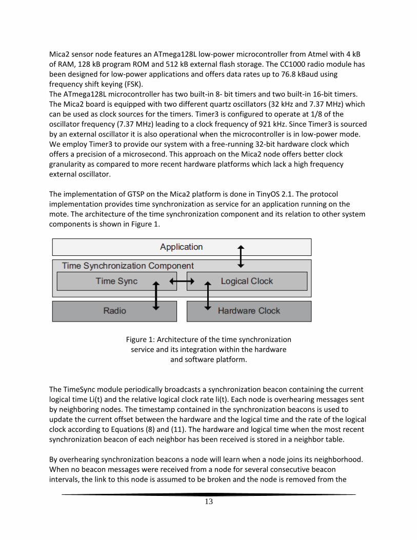
Mica2 sensor node features an ATmega128L low-power microcontroller from Atmel with 4 kB of RAM, 128 kB program ROM and 512 kB external flash storage. The CC1000 radio module has been designed for low-power applications and offers data rates up to 76.8 kBaud using frequency shift keying (FSK). The ATmega128L microcontroller has two built-in 8- bit timers and two built-in 16-bit timers. The Mica2 board is equipped with two different quartz oscillators (32 kHz and 7.37 MHz) which can be used as clock sources for the timers. Timer3 is configured to operate at 1/8 of the oscillator frequency (7.37 MHz) leading to a clock frequency of 921 kHz. Since Timer3 is sourced by an external oscillator it is also operational when the microcontroller is in low-power mode. We employ Timer3 to provide our system with a free-running 32-bit hardware clock which offers a precision of a microsecond. This approach on the Mica2 node offers better clock granularity as compared to more recent hardware platforms which lack a high frequency external oscillator. The implementation of GTSP on the Mica2 platform is done in TinyOS 2.1. The protocol implementation provides time synchronization as service for an application running on the mote. The architecture of the time synchronization component and its relation to other system components is shown in Figure 1.

Figure 1: Architecture of the time synchronization

service and its integration within the hardware and software platform.

The TimeSync module periodically broadcasts a synchronization beacon containing the current logical time Li(t) and the relative logical clock rate li(t). Each node is overhearing messages sent by neighboring nodes. The timestamp contained in the synchronization beacons is used to update the current offset between the hardware and the logical time and the rate of the logical clock according to Equations (8) and (11). The hardware and logical time when the most recent synchronization beacon of each neighbor has been received is stored in a neighbor table. By overhearing synchronization beacons a node will learn when a node joins its neighborhood. When no beacon messages were received from a node for several consecutive beacon intervals, the link to this node is assumed to be broken and the node is removed from the

14

neighbor table. The capacity of the neighbor table is limited by the data memory available on the node. An upper bound for the required capacity is the maximum node degree in the network. However, as long as the resulting network graph stays connected it is possible to ignore synchronization beacons from a specific neighbor. The default capacity of the neighbor table in our implementation is set to 16. Furthermore, the time interval between synchronization beacons can be adapted dynamically. This allows to increase the frequency of beacons during the bootstrap phase or when a new node has recently joined the network. On the other side, if the system is in the steady-state, i.e., all nodes are quite well synchronized to their neighbors, reducing the number of sent beacons can save energy.

3.4 MAC Layer Timestamping Broadcasting time information using periodic beacons is optimal in terms of the message complexity since the neighbor is not forced to acknowledge the message as in sender-receiver synchronization schemes (e.g., TPSN). However, the propagation delay of a message cannot be calculated directly from the embedded timestamps. Exchanging the current timestamp of a node by a broadcast introduces errors with magnitudes larger than the required precision due to non-determinism in the message delay. The time it takes from the point of time where the message is passed to the communication stack until it reaches the application layer on a neighboring node is highly non-deterministic due to various sources of errors induced in the message path. Reducing the main sources of errors by time-stamping at the MAC layer is a well-known approach. The current timestamp is written into the message payload right before the packet is transmitted over the air. Accordingly, at the receiver side the timestamp is recorded right after the preamble bytes of an incoming message have been received. Byte-oriented radio chips, e.g., the CC1000 chip of the Mica2 platform, generate an interrupt when a complete data byte has been received and written into the input buffer. The interrupt handler reads the current timestamp from the hardware clock and stores it in the metadata of the message. However, there exists some jitter in the reaction time of the interrupt handler for incoming radio data bytes. The concurrency model of TinyOS requires that asynchronous access to shared variables has to be protected by the use of atomic sections. An interrupt signaled during this period is delayed until the end of the atomic block. To achieve clock synchronization with accuracy in the order of a few microseconds, it is inevitable to cope with such cases in order to reduce the variance in the message delay. Therefore, each message is timestamped multiple times both at the sender and receiver sides.

15

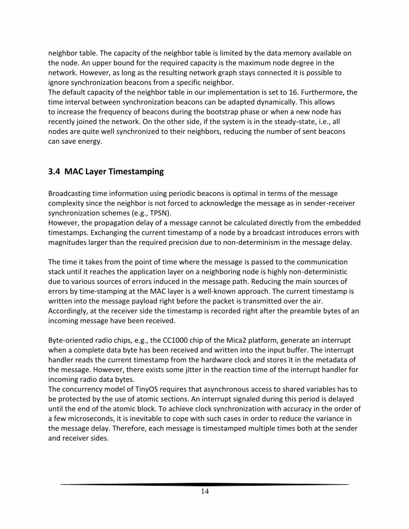
Figure 2: Timestamping at the MAC Layer: An interrupt (solid arrow) is generated

if a complete byte is received by the CC1000 radio chip.

The radio chip generates an interrupt at time bi when a new data byte has arrived or is ready to be transmitted. The interrupt handler is invoked and reads the current hardware clock value at time ti as shown in Figure 2. The time it takes the radio chip to transmit a single byte over the air is denoted by the BYTE_TIME. This constant can be calculated directly from the baud rate and encoding settings of the radio chip. Due to the fact that it takes BYTE_TIME to transmit a single byte, the following equation holds for all timestamps:

(12) Using multiple timestamps, it is hence possible to compensate for the interrupt latency. A better estimation for the timestamp of the i-th byte can calculated as follows:

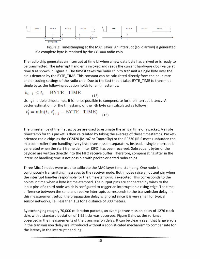
(13) The timestamps of the first six bytes are used to estimate the arrival time of a packet. A single timestamp for this packet is then calculated by taking the average of these timestamps. Packet-oriented radio chips as the CC2420 (MicaZ or TmoteSky) or the RF230 (IRIS mote) unburden the microcontroller from handling every byte transmission separately. Instead, a single interrupt is generated when the start frame delimiter (SFD) has been received. Subsequent bytes of the payload are written directly into the FIFO receive buffer. Therefore, compensating jitter in the interrupt handling time is not possible with packet-oriented radio chips. Three Mica2 nodes were used to calibrate the MAC layer time-stamping. One node is continuously transmitting messages to the receiver node. Both nodes raise an output pin when the interrupt handler responsible for the time-stamping is executed. This corresponds to the points in time when a byte is time-stamped. The output pins are connected by wires to the input pins of a third node which is configured to trigger an interrupt on a rising edge. The time difference between the send and receive interrupts corresponds to the transmission delay. In this measurement setup, the propagation delay is ignored since it is very small for typical sensor networks, i.e., less than 1μs for a distance of 300 meters. By exchanging roughly 70,000 calibration packets, an average transmission delay of 1276 clock ticks with a standard deviation of 1.95 ticks was observed. Figure 3 shows the variance observed in the measurements of the transmission delay. It can be clearly seen that large errors in the transmission delay are introduced without a sophisticated mechanism to compensate for the latency in the interrupt handling.

16

Figure 3: Measurements of the latency in the interrupt handling for the Mica2 node.

3.5 Evaluating performances Evaluating clock synchronization algorithms is always an issue since various performance aspects can be evaluated, e.g., precision, energy consumption, or communication overhead. In this paper, we restrict our evaluation to the precision achieved by the synchronization algorithm. Measuring the instantaneous error between logical clock of different nodes is only possible at a common time instant, e.g., when all nodes can observe the same event simultaneously. A general practice when evaluating time synchronization algorithms for sensor networks is to transmit a message as a reference broadcast. All nodes are placed in communication range of the reference broadcaster. The broadcast message arrives simultaneously at all nodes (if the minimal differences in the propagation delay are neglected) and is time-stamped with the hardware clock. The corresponding logical clock value is used to calculate the synchronization error to other nodes. Two different metrics are used throughout the evaluation in this paper: the Average Neighbor Error measures the average pair-wise differences in the logical clock values of nodes which are direct neighbors in the network graph while the Average Network Error is defined as the average synchronization error between arbitrary nodes. The implementation of GTSP was experimented on a testbench which consists of 20 Mica2 sensor nodes. The nodes were placed in close proximity forming a single broadcast domain. In addition, a base station node is attached to a PC to log synchronization messages sent by the nodes. To facilitate measurements on different network topologies, a virtual network layer is introduced in the management software of the sensor nodes. Each node can be configured with a whitelist of nodes from which it will further process incoming messages, packets from all

17

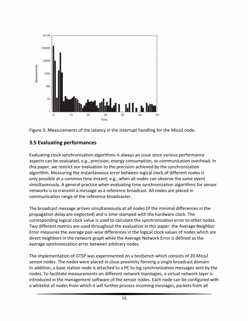
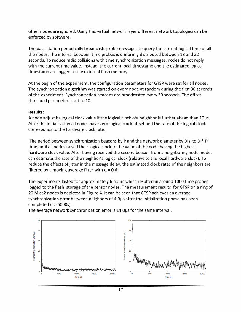
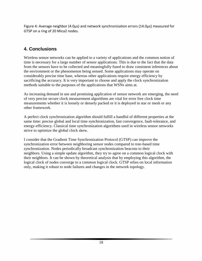
other nodes are ignored. Using this virtual network layer different network topologies can be enforced by software. The base station periodically broadcasts probe messages to query the current logical time of all the nodes. The interval between time probes is uniformly distributed between 18 and 22 seconds. To reduce radio collisions with time synchronization messages, nodes do not reply with the current time value. Instead, the current local timestamp and the estimated logical timestamp are logged to the external flash memory. At the begin of the experiment, the configuration parameters for GTSP were set for all nodes. The synchronization algorithm was started on every node at random during the first 30 seconds of the experiment. Synchronization beacons are broadcasted every 30 seconds. The offset threshold parameter is set to 10. Results: A node adjust its logical clock value if the logical clock ofa neighbor is further ahead than 10μs. After the initialization all nodes have zero logical clock offset and the rate of the logical clock corresponds to the hardware clock rate. The period between synchronization beacons by P and the network diameter by Dis to D * P time until all nodes raised their logicalclock to the value of the node having the highest hardware clock value. After having received the second beacon from a neighboring node, nodes can estimate the rate of the neighbor’s logical clock (relative to the local hardware clock). To reduce the effects of jitter in the message delay, the estimated clock rates of the neighbors are filtered by a moving average filter with α = 0.6. The experiments lasted for approximately 6 hours which resulted in around 1000 time probes logged to the flash storage of the sensor nodes. The measurement results for GTSP on a ring of 20 Mica2 nodes is depicted in Figure 4. It can be seen that GTSP achieves an average synchronization error between neighbors of 4.0μs after the initialization phase has been completed (t > 5000s). The average network synchronization error is 14.0μs for the same interval.

18

Figure 4: Average neighbor (4.0μs) and network synchronization errors (14.0μs) measured for GTSP on a ring of 20 Mica2 nodes.

4. Conclusions

Wireless sensor networks can be applied to a variety of applications and the common notion of

time is necessary for a large number of sensor applications. This is due to the fact that the data

from the sensors have to be collected and meaningfully fused to draw consistent inferences about

the environment or the phenomenon being sensed. Some applications may operate on

considerably precise time base, whereas other applications require energy efficiency by

sacrificing the accuracy. It is very important to choose and apply the clock synchronization

methods suitable to the purposes of the applications that WSNs aims at.

As increasing demand in use and promising application of sensor network are emerging, the need

of very precise secure clock measurement algorithms are vital for error free clock time

measurements whether it is loosely or densely packed or it is deployed in star or mesh or any

other framework.

A perfect clock synchronization algorithm should fulfill a handful of different properties at the

same time: precise global and local time synchronization, fast convergence, fault-tolerance, and

energy-efficiency. Classical time synchronization algorithms used in wireless sensor networks

strive to optimize the global clock skew.

I consider that the Gradient Time Synchronization Protocol (GTSP) can improve the

synchronization error between neighboring sensor nodes compared to tree-based time

synchronization. Nodes periodically broadcast synchronization beacons to their

neighbors. Using a simple update algorithm, they try to agree on a common logical clock with

their neighbors. It can be shown by theoretical analysis that by employing this algorithm, the

logical clock of nodes converge to a common logical clock. GTSP relies on local information

only, making it robust to node failures and changes in the network topology.

19

References [1] Mehdi Saeidmanesh, Mojtaba Hajimohammadi, and Ali Movaghar, “Energy and Distance Based Clustering: An Energy Efficient Clustering Method for Wireless Sensor Networks”, World Academy of Science, Engineering and Technology , USA, Vol 3, 2009

[2] Michael Roche,Time Synchronization in Wireless Networks, 2006

[3] Bharath Sundararaman, Ugo Buy, and Ajay D. Kshemkalyani ,Clock Synchronization for Wireless Sensor Networks: A Survey, March 22, 2005 [4] Prakash Ranganathan, Kendall Nygard, , Department of Computer Science, International Jurnal of UbiComp (IJU), Vol1, No. 2, April 2010 [5] S. Ganeriwal, M. Srivastava, “Timing-sync Protocol for Sensor Networks (TPSN) on Berkeley Motes,” NESL, 2003. [6] D. Mills. Internet Time Synchronization: the Network Time Protocol. IEEE Transactions on Communications, 39(10):1482–1493, Oct 1991. [7] Elson, J.; Girod, L.; Estrin, D. Fine-grained network time synchronization using reference broadcasts. In Procedings. of the Fifth Symposium on Operating System Design and Implementation, Boston, MA, USA, Dec. 2002. [8] R. Fan and N. Lynch. Gradient Clock Synchronization. In PODC ’04: Proceedings of the twenty-third annual ACM symposium on Principles of distributed computing, 2004. [9] J. Sallai, B. Kusy, A. Ledeczi, and P. Dutta. On the scalability of routing integrated time synchronization. 3rd European Workshop on Wireless Sensor Networks (EWSN), 2006. [10] S. Ganeriwal, R. Kumar, and M. B. Srivastava. Timing-sync Protocol for Sensor Networks. In SenSys ’03: Proceedings of the 1st international conference on Embedded networked sensor systems, 2003. [11] M. Maroti, B. Kusy, G. Simon, and A. Ledeczi.The Flooding Time Synchronization Protocol. In SenSys ’04: Proceedings of the 2nd international conference on Embedded networked sensor systems, 2004. [12] G. Werner-Allen, G. Tewari, A. Patel, M. Welsh, and R. Nagpal. Firefly-Inspired Sensor Network Synchronicity with Realistic Radio Effects. In SenSys ’05: Proceedings of the 3rd international conference on Embedded [13] T. K. Srikanth and S. Toueg. Optimal Clock Synchronization. J. ACM, 34(3), 1987. [14] R. Fan and N. Lynch. Gradient Clock Synchronization. In PODC ’04: Proceedings of the twenty-third annual ACM symposium on Principles of distributed computing, 2004. [15] W. Su, I. Akyildiz, Time-Diffusion Synchronization Protocols for Sensor Networks, IEEE/ACM Transactions on Networking, 2005, in press. [16] Q. Li and D. Rus. Global Clock Synchronization in Sensor Networks, Proc. IEEE Conf. Computer Communications (INFOCOM 2004), Vol. 1, pp. 564–574, Hong Kong, China, Mar. 2004. [17] Philipp Sommer , Roger Wattenhofer Gradient Clock Synchronization in Wireless Sensor Networks