Download pdf - Tracking highly maneuverable targets with unknown behavior

Tracking Highly Maneuverable Targets WithUnknown Behavior

CHAD SCHELL, MEMBER, IEEE, STEPHEN P. LINDER, MEMBER, IEEE, AND

JAMES R. ZEIDLER, FELLOW, IEEE

Invited Paper

Tracking of highly maneuvering targets with unknown behavioris a difficult problem in sequential state estimation. The perfor-mance of predictive-model-based Bayesian state estimators dete-riorates quickly when their models are no longer accurate or theirprocess noise is large. A data-driven approach to tracking, the seg-menting track identifier (STI), is presented as an algorithm that op-erates well in environments where the measurement system is wellunderstood but target motion is either or both highly unpredictableor poorly characterized. The STI achieves improved state estimatesby the least-squares fitting of a motion model to a segment of datathat has been partitioned from the total track such that it repre-sents a single maneuver. Real-world STI tracking performance isdemonstrated using sonar data collected from free-swimming fish,where the STI is shown to be effective at tracking highly maneu-vering targets while relatively insensitive to its tuning parameters.Additionally, an extension of the STI to allow its use in the mostcommon multiple target and cluttered environment data associationframeworks is presented, and an STI-based joint probabilistic dataassociation filter (STIJPDAF) is derived as a specific example. TheSTIJPDAF is shown by simulation to be effective at tracking a singlefish in clutter and through empirical results from video data to beeffective at simultaneously tracking multiple free-swimming fish.

Keywords—Probabilistic data association, state estimation,tracking.

I. INTRODUCTION

A common application of sequential state estimationis the tracking of targets as they move through a sensor’sfield of view. Many of the filters commonly used for target

Manuscript received February 13, 2003; revised October 28, 2003. Thismaterial is based in part upon work supported under a National ScienceFoundation Graduate Fellowship.

C. Schell was with the San Diego Electrical and Computer EngineeringDepartment and the Scripps Institution of Oceanography, University of Cal-ifornia, La Jolla, CA 92093 USA. He is now with Rincon Research Corpo-ration, Tucson, AZ 85711 USA (e-mail: [email protected]).

S. P. Linder is with the Department of Computer Science, Dartmouth Col-lege, Hanover, NH 03755-3510 USA (e-mail: [email protected]).

J. R. Zeidler is with the San Diego Electrical and Computer EngineeringDepartment, University of California, La Jolla, CA 92093 USA (e-mail: [email protected]).

Digital Object Identifier 10.1109/JPROC.2003.823151

tracking, such as the Kalman filter and its relatives, arepredictive model-based Bayesian state estimators. Thesefilters achieve improved state estimates through the use ofa predictive model that describes the evolution of the targetstate through time. The model consists of a state transitionfunction that describes the evolution of the state in theabsence of (unknown) external inputs, and a process noisethat represents unknown changes to the state not describedin the state transition function.

However, state evolution is often not easily modeled in apredictive fashion. This can happen either when the systembeing studied is not well understood, or when the randomchanges in the state are large enough to dominate the pre-dictable changes. In these situations predictive filters canbecome ineffective and an alternative method is required,one that does not rely on prediction. An alternative is touse parameter estimation or curve fitting techniques to es-timate the target state directly from the data. In order to usethis approach with a relatively simple state vector and fittingfunction, the data must be broken into segments over whichthe simple fitting function can adequately describe the data.Thus, the problem now consists of two parts, segmenting thedata and then estimating the state, or the parameters, of theindividual segments.

This paper demonstrates the performance advantages ofone such data-driven approach to tracking highly maneuver-able targets with unknown behavior: the segmenting trackidentifier (STI), first introduced by Linder [1]. The STI’s ad-vantages are demonstrated by comparison against Kalmanand extended Kalman filters (EKFs) for the tracking of free-swimming fish. Additionally, an extension of the STI algo-rithm is presented, which enables its use in the commondata association frameworks for multiple target tracking, andan STI-based joint probabilistic data association filter (STI-JPDAF) is developed as a specific example. The effective-ness of the STIJPDAF is demonstrated using simulations andempirical results from fish-tracking experiments.

0018-9219/04$20.00 © 2004 IEEE

558 PROCEEDINGS OF THE IEEE, VOL. 92, NO. 3, MARCH 2004

II. SEGMENTING TRACK IDENTIFIER

The STI is a data-driven tracking algorithm that achievesimproved state estimates by partitioning the track data intosegments which contain only a single maneuver and thenperforming least-squares fitting of the motion model to eachtrack segment. It is similar in some ways to algorithms de-signed to recognize curves and lines in images and freehanddrawings [2]–[4]. However, these image processing methodsgenerally rely on a high sampling density and relatively lowmeasurement noise as their purpose is to reconstruct or rec-ognize elements of images which already look approximatelylike lines or arcs, while the STI algorithm is designed to op-erate not only in low-noise, high data rate situations, but alsoin low-noise, low data rate and high-noise, high data rate sit-uations.

As the STI is a data-driven rather than a predictivealgorithm, no process noise is required to handle targetmaneuvers. Maneuvers are represented by a segmentationof the data, and segmentation decisions are based only onknowledge of the system measurement errors, a quantitythat is very likely known regardless of the type of targetbeing tracked. Additionally, segmentation also allows rapidresponse to large abrupt maneuvers as it makes a cleanbreak from the previous segment, which is helpful in lowdata rate environments where predictive filters may be slowto respond to such maneuvers. However, one drawback tothe STI’s lack of prediction is that STI in its simplest formcannot be easily used in the most common data associationframeworks for tracking in clutter or for tracking multipletargets.

This section presents the original single-target STI algo-rithm, and as a specific example details the development ofa motion model for a target performing constant speed co-ordinated turns. After presenting the original single-targetversion of the STI, an extension to the STI algorithm thatcomputes a measurement prediction and its covariance is pre-sented. This extension allows the STI to now be used in manyof the common data association frameworks including as-signment methods and multiple hypothesis tracking. Finally,as an example, the STIJPDAF is developed in detail. A prob-abilistic data association (PDA) algorithm was chosen as theexample because using the STI in a PDA algorithm requiressome additional consideration to support the two-way com-munication required between the PDA algorithm and the STI.

A. STI Algorithm

The STI algorithm dynamically partitions a target trackinto segments, , where is an index that startsat one and grows as the algorithm determines new segmentsare needed. The sequential target state is estimated by recur-sively calculating the segment parameter vectors, ,that minimize the pairwise sums of the segment least-squarescost functions . A recursive, pairwise minimization isused in place of a global minimization to keep the problemcomputationally tractable.

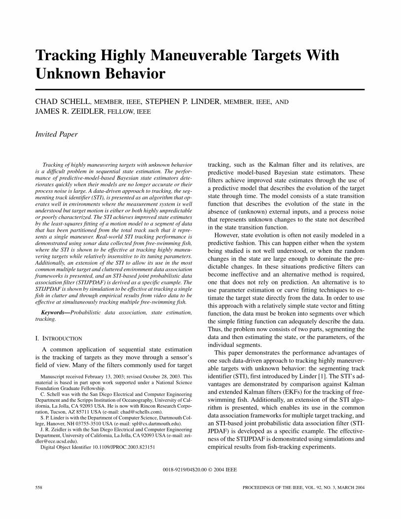
Fig. 1. STI fit and segmentation stage flowchart.

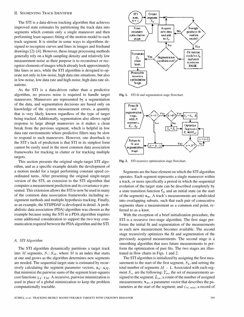
Fig. 2. STI recursive optimization stage flowchart.

Segments are the base element on which the STI algorithmoperates. Each segment represents a single maneuver withina track, or more specifically a period in which the sequentialevolution of the target state can be described completely bya state transition function and an initial state (at the startof the segment) . A track’s measurements are subdividedinto overlapping subsets, such that each pair of consecutivesegments share a measurement as a common end point, re-ferred to as a knot.

With the exception of a brief initialization procedure, theSTI is a recursive two-stage algorithm. The first stage per-forms the initial fit and segmentation of the measurementsas each new measurement becomes available. The secondstage recursively optimizes the fit and segmentation of thepreviously acquired measurements. The second stage is asmoothing algorithm that uses future measurements to per-form the optimization of past fits. The two stages are illus-trated in flow charts in Figs. 1 and 2.

The STI algorithm is initialized by assigning the first mea-surement to the start of the first segment, , and setting thetotal number of segments . Associated with each seg-ment are the following: , the set of measurements as-signed to the segment; , a count of the number of assignedmeasurements; , a parameter vector that describes the pa-rameters at the start of the segment; and , a record of

SCHELL et al.: TRACKING HIGHLY MANEUVERABLE TARGETS WITH UNKNOWN BEHAVIOR 559

the lowest root-mean-squared fitting error achieved for thesegment. Note that the values of and are unde-fined until the segment has actually been fit to the motionmodel, which occurs in the fit and segmentation stage.

1) Fit and Segmentation Stage: Each new measurementis added to the current segment . If, after adding the mea-surement, , where is the minimum numberof points required to perform a fit to the motion model, thealgorithm returns to the start of this stage. Otherwise, the pa-rameter vector is estimated to minimize the least-squarescost function

(1)

where is the vector valued function thatcalculates both the continuity knot costs between and

and the measurement residuals for for a given. The continuity knot costs maintain continuity of mo-

tion between two segments. For segment , the knot costsare identically zero as there is no previous segment . Theroot-mean-squared error (RMSE), is alsocalculated, where is the length of the vector , which isequal to the dimension of the measurement vector times ,plus the dimension of the knot costs. Each time the segmentis fit, is updated as

otherwise (2)

This add-and-fit procedure is repeated for each new mea-surement until a segmentation condition is met. A segmenta-tion condition occurs when any of the following are true:

(3)

where is the measurement noise standard deviation, andand are tuning parameters that determine the thresh-

olds used for segmentation. The value represents theroot-mean-squared measurement residual for the last mea-surements, and is helpful in detecting break conditions inlong segments, where the poor fit from new measurementsafter a maneuver is obscured in by the averaging acrossthe entire length of the segment. The value is also a tuningparameter of the algorithm, but it is restricted to integers be-tween one and ; otherwise, it would not exist for all fitsegments as the segments could be shorter than the tail.

Once a segmentation condition has occurred, the segmentis terminated and the most recently added measurement

is removed from the segment. A new segment isstarted, and the last measurement of and the measure-ment that caused the segmentation condition are assignedas the first two measurements of . The shared mea-surement is the location of the knot between segmentsand . The algorithm then proceeds to the recursiveoptimization stage.

2) Recursive Optimization Stage: This stage recursivelyoptimizes the fit and segmentation of past segments, per-

forming the optimization on a pair of segments at one time.The optimization requires that the number of fitted segmentsbe and begin with segment ,where is the optimization depth, the maximum number ofprevious segments to reoptimize. If , no optimizationis performed, and the algorithm returns to the start of the fitand segmentation stage with .

The optimization algorithm works as follows. Startingwith segment , form , the union of themeasurements from and . The set willcontain measurements, as theknot will only appear once in the union. Define the notation

as the subset of containing the ththrough th measurements when listed in ascending timeorder of arrival. The goal of the algorithm is to replaceand by the optimal segmentation, and , ofthe combined data set defined as the knot location

, and the optimized segment parameter vectors,and , such that the cost

(4)

is minimized subject to the constraint that, where is the same as in (1). After

the optimal segmentation has been found, and arereplaced by their optimal counter parts, and the algorithmproceeds to optimize the next pair of segments, starting with

(one of the segments just replaced). This loopcontinues up to . After the optimization loopis completed, the algorithm returns to the start of the fit andsegmentation stage with .

Because the STI optimization procedure operates onlyon pairs of segments, it is expected that large optimizationdepths will produce diminishing returns because the locationof the knots between pairs of segments will tend to settleto constant values for segments that have been reoptimizedmultiple times. Experience with the STI optimizationalgorithm has shown that there is practically no change forvalues of , so is suggested as a constant andwas used in this study.

3) STI Motion Models and Knot Costs: This sectionpresents the format for STI motion models. They consistof a measurement generating function, , and acontinuity knot cost function . These functionsare used together to form the STI cost function

(5)

where is the th measurement of the set , andis the elapsed time of the same measurement relative

to the first measurement in . [For example, .]As a specific example, the constant speed coordinated turnmodel used in a study of fish behavior [5] is presented.


The minimum number of measurements required to com-pute a fit for this model is , and the parametervector estimated for each segmentconsists of the target’s position and course atthe start of the segment, and the target’s speed and turnrate , both constant throughout the segment. The mea-surement generating function is given by

(6)

which in the case of is the time parameterized equa-tion of an constant speed, constant turn rate arc, and in thecase of is the time parameterized equation of a con-stant speed straight line segment. The continuity knot costfunction is

(7)

where is the knot cost multiplier, a tuning factor that af-fects how important continuity in position and heading at theknots is relative to the fit between the motion model and themeasurements. The factor insures that the pro-portional weight of the knot cost remains relatively constanteven as the total length of the two segments increases.is the distance between the positions at the start of andthe end of , and is the difference in course, mea-sured in radians and ranging from zero (same course) to(directly opposite course) radians.

B. STI Data Association

The required modifications to the single-target STI trackerfor its use in the most common data association frameworksare presented in this section. The first modification, the cal-culation of the measurement prediction for the STI is trivial,as the measurement generating function, , of theSTI model already serves this purpose. All that is required isto extend the time of the final measurement in the segment

, which is measured relative to the time of the startof the segment, to the time of the desired measurement pre-diction, . Then the predicted measurement is given by

(8)

The second modification, calculation of the measurementprediction covariance, is more difficult, but with the assump-tion that the STI is an unbiased estimator one can generate a

covariance for the STI state parameters for a given segmentusing the Cramer–Rao lower bound (CRLB). The measure-ment prediction covariance is then generated using the CRLBand a process noise that characterizes the possible maneuversof the target.

The CRLB represents the lowest possible covariancethat can be obtained using any filter for a given set ofmeasurements. Although it is used here to generate the statecovariance for a segment, it is not meant to imply that theSTI algorithm actually obtains this lower bound. It is simplyused as a means of generating a state covariance that can becompared relative to the state covariance of segments fromother tracks.

The process noise for the STI algorithm is added tothe measurement prediction covariance rather than thestate covariance, because the process noise represents theuncertainty in a target’s predicted location that comesfrom target behavior between the last measurement and theprediction time. Without the process noise, the covarianceestimate would approach zero with increasing information(increasing segment length), resulting in a zero-volumesearch location for the next measurement. The use of theprocess noise to model small unpredictable motions is notimportant to the underlying STI algorithm as it does not usethe state covariance in fitting and segmentation.

Using the definition of the CRLB, the minimum statecovariance for the latest segment, , with estimatedparameter vector , representing the state at the start ofthe segment is

(9)

where is the true target parameter vector (unknown forreal data sets). is the Fisher information matrix (FIM) givenby

(10)

with the expectation carried out over , the set of mea-surements associated with the segment. is thelikelihood function of , defined as

(11)

where is the probability of given .is the log likelihood of .

Given a measurement noise vector, , assumed to bea zero-mean Gaussian white sequence with known covari-ance matrix , represent the actual noisy measure-ment as

(12)


The likelihood function is then

(13)

and the log likelihood of , dropping the unnecessary nor-malization constants represented by in (13), is

(14)

Inserting (14) into (10) and using the whiteness of the mea-surement errors , one reaches the formula for the FIMas shown in (15), at the bottom of the page.

Taking the inverse of (15) evaluated at pro-vides the absolute minimum state covariance for giventhe set of measurements . Despite the fact that this boundis practically unrealizable for any filter operating on a realdata set, computing this bound at the estimated state pro-vides a relative estimate of the covariance of the segment’sstate vector. Consequently, in the implementation of data as-sociation algorithms using STI, the estimated state covari-ance of at time is given by , whereis calculated according to (15).

With the state covariance calculated, the measurement pre-diction covariance at time , can be calculated as

(16)

where

(17)

is the measurement prediction process noise, which repre-sents the uncertainty in the measurement prediction resultingfrom possible changes in the target motion parameters be-tween the last measurement time and the time ofthe predicted measurement . is the target stateat the end of the segment (rather than the beginning).

is the elapsed time between the last mea-surement and the time of the desired prediction. The expec-tation in (17) is taken over the elements of the process noisevector , which are random variables that characterize the

possible changes in the target state motion parameters duringthe interval . The function is the be-havior modified measurement generating equation that cal-culates the predicted measurement for a given value of , orin other words it is the function that expresses the effects ofthe change in state on the predicted measurements.

Calculation of can be difficult for nonlinear mo-tion models, often requiring the evaluation of complicated in-tegrals with no closed form solution. However, if the changesin target state are limited to entering only as additive impulsefunctions added at the last measurement time , suchas an instantaneous change in turn rate or speed, and the ele-ments of are assumed to be zero-mean Gaussian variableswith known covariance matrix can be calcu-lated simply as

(18)

As the process noise is a design parameter to keep the pre-diction window large enough to cover target maneuvers (andnot an exact representation of knowledge about the target’smotion), the simplified computation of (18) is reasonable inmany cases.

This completes the evaluation of the measurementprediction and its covariance, but there is still one moresmall change required to the STI in order to use it in dataassociation frameworks. The STI normally waits until thereare enough measurements in a segment to fit the desiredmotion model before estimating the segment’s parameters.Thus, when the current segment has too few points to fit themotion model, no measurement prediction or covariancewould be available. To compensate for this, a simpler motionmodel must be fit for segments that do not have enoughmeasurements to fit the ultimate desired motion model. Agood model for this purpose is a simple straight line constantvelocity model, in whatever dimensions is appropriate forthe data set (one-dimensional, two-dimensional, etc.), as thismodel can be fit for two measurements, and there are alwaysat least two measurements in a segment after the track hasbeen initialized.

With this modification, the STI algorithm can now be usedin data association algorithms that only require one-waycommunication from the tracking filter to the associationalgorithm, such as most assignment methods and multiplehypothesis tracking [6]. Additional work is required to usethe STI algorithm in PDA algorithms because storing themeasurement uncertainty in a way that will be recognizedby the STI is required. A method for accomplishing this ispresented in the following section.

(15)


C. STI Probabilistic Data Association

Implementation of a PDA algorithm using the STIrequires some special consideration. Typically, PDA algo-rithms using model-based Bayesian state estimators as theirtracking filters generate a synthetic innovation and associ-ated covariance from a track’s predicted measurement andall the measurements possibly associated with the track, andthen return this to the tracking algorithm for use in its updateprocedure [6]. As the synthetic innovation has a highercovariance than that of a single, unambiguously assignedmeasurement, its use in the update process increases thecovariance of the Bayesian state estimate.

As the STI algorithm does not use or store a state covari-ance matrix, the uncertainty cannot be passed back to theSTI in this fashion. This section presents a method to repre-sent the increased uncertainty from multiple measurementsand less than unity probability of detection (data associa-tion uncertainty) in an STI-based PDA algorithm. The syn-thetic innovation is replaced by a synthetic measurement andits covariance, essentially the effective measurement covari-ance. This effective measurement covariance is stored withthe measurement for use in computing the measurement pre-diction covariance.

This procedure is illustrated by presenting the derivationof the STIJPDAF in its entirety. This presentation closelyparallels the presentation of the Kalman filter-based JPDAFalgorithm of Bar-Shalom and Li [6]. The STIJPDAF makesthe following assumptions.

1) There are a known number of targets currently undertrack.

2) The past is summarized by the information in the STIfilters for the active tracks, including the associatedeffective measurement covariances.

3) The true measurements are Gaussian distributedaround the measurement predictions with knowncovariance matrix .

4) The underlying model of the current STI segment foreach target is true and correct.

The STIJPDAF computes the measurement to target asso-ciation probabilities jointly for all targets, and does so onlyfor the current measurement time . The joint associationprobabilities are generated by computing the probabilities forall feasible joint association events. A feasible joint associa-tion event is one where the following conditions are met.

1) Each measurement is associated with at most onetrack.

2) Each track has at most one measurement associatedwith it.

3) The measurement associated with each track lieswithin that track’s validation gate.

The last assumption exists to eliminate the evaluation ofhighly unlikely tracks. Given a track with predicted measure-ment and measurement prediction covariance , a mea-surement falls inside the track validation gate when

(19)

for a given chosen such that the probability of a target lyingin the gate is a desired value.

Given a set of measurements at time , the proba-bility of a particular event is

(20)

where is the number of tracks, is the sensor obser-vation volume, and is the probability of detection fortrack . The quantity is a binary track detection indi-cator, whose value is one if track is detected in , andzero otherwise, and

(21)

is the number of measurements not originating from a track.The probability mass function describes the proba-

bility of observing a given number of clutter (non-target-orig-inated) measurements. Typical distributions for areeither the Poisson distribution

(22)

which is characterized by the clutter density level , or thediffuse prior distribution of [7], , where is anunimportant constant that cancels out when the diffuse prioris used. The diffuse prior represents a situation where theclutter density is unknown; it is also referred to as the un-informative prior.

The function is the likelihood function of the mea-surement defined by (23), assuming that false alarm mea-surements are uniformly distributed within the observationvolume

is associated with

track in event

is a false alarm in event (23)

where is the probability of observing valuefrom a Gaussian distribution with mean and covariancematrix .

The normalization constant in (20) is chosen such thatthe probabilities of the feasible joint events, representing amutually exclusive and exhaustive set of the possible dataassociations, sum to one

(24)

With the calculation of the probabilities of the joint eventscompleted, for each track calculate a set of weights


which represent the probability that measurement is asso-ciated with the track . Also calculate , the probability thetrack was not detected at time . These weights are calcu-lated as

(25)

where the value is a binary track to data associationindicator equal to one if measurement is associated withtrack in event , and zero otherwise.

Up to this point, the STIJPDAF is exactly the same asthe Kalman filter-based joint PDA filter (JPDAF), but nowinstead of calculating a synthetic innovation and its covari-ance for each track, and then performing the Kalman filterupdate procedure, the STIJPDAF will calculate a syntheticmeasurement and the effective measurement covariance foreach track. It will then call the STI algorithm to perform thefit and segmentation stage with the synthetic measurement asthe latest measurement. For each track , calculate the syn-thetic measurement and its covariance as follows:

(26)

(27)

The synthetic measurement and its covariance are storedwith the track, and are used as and in (15)when for purposes of computing the segment statecovariance. Otherwise, the original implementation of theSTI algorithm remains unaltered, with used as the mea-surement and ignored.

Although it is possible to use as a weighting coef-ficient during the STI least-squares fitting operation, effec-tively reducing the importance given to measurements thathave a high degree of uncertainty, there are drawbacks tosuch an option. When target maneuvers are large, weightingthe synthetic measurement will reduce the STI’s ability torespond to changes in target motion, as measurements afterinitial maneuver onset will likely have a large effective mea-surement covariance as the spread of the means between thepredicted and actual measurement will be large. This largecovariance will reduce the effect the measurement has on in-creasing the model fitting residual and possibly prevent theSTI algorithm from properly detecting the need for segmen-tation, as the segmentation criteria rely on the increase in fit-ting residual caused by target maneuvers. Essentially, usingthe effective measurement covariance in this way eliminatesthe STI’s independence from a process noise. Additionally,scaling the measurement residuals makes it more difficult to

compensate for the scaling of knot costs versus measurementfitting costs because of the ever-changing weights of the mea-surement residuals.

III. SINGLE FISH-TRACKING PERFORMANCE EVALUATION

WITH PERFECT DATA ASSOCIATION

In this section the performance of the STI at tracking free-swimming fish is compared against the performance of aKalman filter, a Kalman smoother, and an EKF. First somebackground on the particulars of the fish-tracking problemand the performance metrics used in the evaluation are pre-sented. Next the experimental setup that generated the datasets and the data sets themselves are described, followed bya description of the algorithms tested and the tuning parame-ters of each algorithm. Finally, the results of the comparisonare presented and discussed.

A. Fish-Tracking Background and Performance Metrics

Tracking fish for the purposes of ecological studies pro-vides an example of a difficult tracking problem with char-acteristics not commonly encountered when tracking man-made systems or objects. The goal in these ecological studiesis to develop increased understanding of fish behavior and torepresent that behavior in a simple fashion that lends itselfto behavior classification, statistical analysis, and insertioninto forward models of fish behavior and energetics. Unfor-tunately, the behavior that one wishes to learn, such as fishswimming patterns and maneuver levels, is generally an im-portant input into the models used in sequential state esti-mation algorithms, and its lack of availability requires us totrack targets with unknown behavior. This means that anyalgorithms that are used must be able to function withoutusing a priori information of target behavior (such as ma-neuver-based process noise levels).

The tracking problem is further complicated by the ex-treme maneuverability of free-swimming fish, and the needfor very accurate swimming speed and acceleration estimatesto accurately estimate fish energy expenditure. As an ex-ample of fish maneuvering capabilities, Fig. 3 illustrates thefish horizontal swimming speed and turn rate cumulative dis-tribution functions for the data used in the study presentedin this section. It shows that fish are capable of turn ratesexceeding 100 /s. To put this number in perspective, con-sider the turn capabilities of aircraft, which are limited by theforces involved in maneuvering at high velocities. An aircraftmoving at 300 m/s, a value commonly used in aircraft sim-ulations [8], [9], experiences a force of three times the pullof gravity (3 g’s) when turning at only 5.9 /s. Even at 10 g’s,pushing the limits of aircraft and their pilots, the turn rate at300 m/s is only 19 /s. Additionally, fish are capable of burstsof very high linear acceleration, several times their averageswimming speed, and they can come to a dead stop or swimbackward. Very highly maneuvering targets such as these canpresent problems for predictive-model-based algorithms be-cause high process noise levels are required to represent thehigh uncertainty in motion created by the maneuverability,and a large process noise places most of the emphasis on


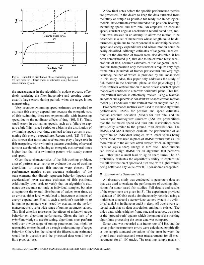
Fig. 3. Cumulative distribution of: (a) swimming speed and(b) turn rates for 100 fish tracks as estimated using the stereovideo-camera system.

the measurement in the algorithm’s update process, effec-tively rendering the filter inoperative and creating unnec-essarily large errors during periods when the target is notmaneuvering.

Very accurate swimming speed estimates are required toestimate fish energy expenditure because the energetic costof fish swimming increases exponentially with increasingspeed due to the nonlinear effects of drag [10], [11]. Thus,small errors in estimating speeds, such as a failure to cap-ture a brief high-speed period or a bias in the distribution ofswimming speeds over time, can lead to large errors in esti-mating fish energy expenditure. Recent work [12]–[14] hasalso shown that turns and accelerations play a large role infish energetics, with swimming patterns consisting of severalturns or accelerations having an energetic cost several timeshigher than that of a swimming pattern with steady courseand speed.

Given these characteristics of the fish-tracking problem,a set of performance metrics to evaluate the use of trackingalgorithms to process fish motion were chosen. Theperformance metrics stress accurate estimation of thestate elements that directly represent behavior (speeds andaccelerations) over accurate estimates of fish positions.Additionally, they seek to verify that an algorithm’s esti-mates are accurate not only at individual samples, but alsoat capturing the overall distribution of values over time, asan error at either level would lead to inaccurate estimates ofenergy expenditure. Finally, each algorithm’s sensitivity toits tuning parameters was tested by evaluating the perfor-mance metrics over a wide range of tuning parameter values.This final criterion represents the effects of unknown targetbehavior on algorithm performance. Given the lack of apriori knowledge to use for tuning, algorithms must performwell over a wide range of tuning parameters that might bereasonably chosen based on a rough understanding of targetbehavior. Otherwise, the value of the filtered state estimateswould be in question and the processed data would be oflittle practical use.

A few final notes before the specific performance metricsare presented. In the desire to keep the data extracted fromthe study as simple as possible for ready use in ecologicalmodels, state estimates were limited to fish position, heading,swimming speed, and turn rate. An emphasis on constantspeed, constant angular acceleration (coordinated turn) mo-tions was stressed in an attempt to allow the motion to bedescribed as a set of maneuvers whose length could be de-termined (again due to the exponential relationship betweenspeed and energy expenditure) and whose motion could beeasily classified. Although estimates of tangential accelera-tions (in the direction of travel) were also desirable, it hasbeen demonstrated [15] that due to the extreme burst accel-erations of fish, accurate estimates of fish tangential accel-erations from position only measurements require very highframe rates (hundreds of frames per second) and very highaccuracy, neither of which is provided by the sonar usedin this study. Also, this paper only addresses the study offish motion in the horizontal plane, as fish physiology [13]often restricts vertical motion to more or less constant speedmaneuvers confined to a narrow horizontal plane. This lim-ited vertical motion is effectively tracked using a Kalmansmoother and a piecewise constant white acceleration motionmodel [7]. For details of the vertical motion analysis, see [5].

Five performance metrics were used to evaluate algorithmperformance: RMSE for position and speed estimates,median absolute deviation (MAD) for turn rate, and thetwo-sample Kolmogorov–Smirnov (KS) test probabilitiesthat the estimated speed and turn rate distributions werestatistically similar to the ground truth distributions. TheRMSE and MAD metrics evaluate the performance of analgorithm on individual samples, with lower values beingbetter. MAD was used in place of RMSE for turn rate as it ismore robust to the outliers often created when an algorithmleads or lags a sharp change in turn rate. These outlierscan create a high RMSE for an algorithm that performswell other than a small lead or lag on sharp turns. The KSprobability evaluates the algorithm’s ability to capture theoverall distribution of speed and turn rate, with higher valuesbeing better and any value over 0.01 considered acceptable.

B. Experimental Setup and Data

A laboratory study was conducted to generate a data setthat was used to evaluate the performance of tracking algo-rithms for sonar-based fish studies. Full details and resultsof the experiment are given in [5]. The experiment provideda data set of 100 fish tracks simultaneously recorded using amultibeam sonar and a stereo video-camera system in a cylin-drical tank 5 m in diameter and 3 m deep. All tracks were se-lected such that no data association ambiguity existed. Thevideo data, with its higher frame-rate and accuracy, was usedas the “ground truth” against which the output of the trackingalgorithms processing the sonar data was compared.

Sonar data was recorded at a frame rate of 4 Hz, and thesonar polar measurement errors were calculated empiricallyas the sample standard deviations of the error between theground truth estimates and sonar measurements for all mea-surements for all 100 tracks. The resulting sample means


and standard deviations are cm, cmfor range, for bearing angle,and for elevation angle. Sonarmeasurements were converted to Cartesian coordinates usingthe unbiased conversion technique of [16], which also calcu-lates an appropriate Cartesian measurement error covariancematrix given the above polar measurement standard devia-tions. These converted measurements and associated covari-ance matrices were supplied to the tracking algorithms.

The video data was recorded at a 29.97-Hz frame rate,and had a mean spherical distance error of 1.08 cm witha standard deviation of 0.70 cm. “Ground truth” referencevalues were obtained by smoothing the video positionmeasurements along each Cartesian axis with a fifth orderSavitzky–Golay filter [17] over 29 data points, and thencalculating velocities along each Cartesian axis by differen-tiating the smoothed video positions. Horizontal speed wascalculated as the absolute vector sum of the two Cartesianvelocities. Target course was calculated as the arctangent ofthe two Cartesian velocities, and these course estimates wereagain smoothed with a fifth-order Savitzky–Golay filter thendifferentiated to produce the turn rate estimates. Finally, allestimates were down-sampled to 4 Hz to correspond to thesonar measurements.

C. Algorithms and Tuning Parameters

This section provides a brief description of the modelsused in the Kalman filter algorithms used in this comparison,as well as a description of the tuning parameters associatedwith these algorithms and the STI. For full details on the al-gorithms and models, see [5].

The Kalman filter and smoother both used the piecewiseconstant white acceleration model of [7]. This model filtersmotion along each Cartesian axis independently and as-sumes that the motion is constant velocity motion perturbedby small random accelerations which are piecewise constantduring each sampling period. The accelerations enter byway of the process noise, which is assumed to be zero-mean,white, Gaussian distributed with known covariance. Thesmoother was implemented following the presentation of[18], and the smoothing was performed over the entirelength of the track. The Kalman filter and smoother bothhave only one tuning parameter, the standard deviation ofthe process noise acceleration for each Cartesian axis, setidentically equal in this analysis. It was varied from 1 cm/sto 100 cm/s in 1-cm/s increments.

The EKF used a variation of the polar constant speed co-ordinated turn model of [19]. The original model of [19] as-sumed the target did not change speed and, thus, supplied aprocess noise only for angular acceleration, while our modelused two independent process noise accelerations, tangen-tial and angular, to allow for changes in both speed and turnrate. The standard deviations of these two process noise ac-celerations are the tuning parameters of the EKF. The an-gular acceleration process noise was swept from 10 /s to100 /s in 10 /s increments, and the tangential accelerationprocess noise was swept from 1 cm/s to 50 cm/s in 1-cm/sincrements.

The STI used the constant speed coordinated turn modeldescribed in Section II. A special consideration for the STIalgorithm was the choice of the noise standard deviationused in the STI break condition computations of (3), giventhat was not actually constant because the base sonar mea-surements were in spherical coordinates. The value used wasthat generated by a measurement which lies at the middlerange value of the field of view, 337 cm, and at the middleof the angular limits, 4 in both bearing and elevation, onthe basis that this represents approximately the midpoint ofthe Cartesian errors. Specifically, the Cartesian measurementerror covariance for a measurement at this position was cal-culated using the unbiased spherical to Cartesian coordinatedconversion algorithm [16], and the diagonals of the covari-ance matrix were then used as the measurement variances foreach Cartesian axis. The radial measurement standard devi-ation was used, cm.

The STI was evaluated against the four tuning parametersmentioned in Section II. As these tuning parameters do nothave physical analogs like the Kalman tuning parameters,the reasoning behind the selection of their values will be dis-cussed. The first tuning parameter is the noise threshold ;it should typically be near one so that the segmentation oc-curs when the fitting cost is worse than expected accordingto the measurement noise standard deviation . Varying itgives an idea of the sensitivity to errors in the choice of noisethreshold. was varied from 0.6 to 2 in increments of 0.2.

Next is the RMSE ratio , which is used to tune tracksegmentation based on the ratio of the current fit to the bestprevious fit (when the segment had fewer data points asso-ciated with it). If is chosen too large, most segmentationwill occur because of the break condition. If is closeto one (it must be greater than or equal to one or else seg-mentation will occur for situations where the current fit isbetter than past fits), segmentation will occur too frequentlyas slightly better previous fits will result in a new segment.

was tested for values of two, three, and four.The third tuning parameter is the tail length . deter-

mines the sensitivity to new maneuvers when the current seg-ment is long. As is limited to being an integer between oneand the minimum number of measurements required to fit themodel, it was natural to sweep over the allowable values,

.Finally, there is the knot cost tuning parameter . de-

termines the relative importance of knot continuity versus thefitting of the measurements within each segment. Choosingvery small values implies that continuity is of little impor-tance, whereas choosing very large values is impractical, as itforces all segments to be continuous and essentially ignoresthe measurements to fit a continuous curve. was sweptfrom 0 to 2 in increments of 0.2.

D. Single Fish-Tracking Performance Evaluation Results

The results of the performance evaluation are presentedas a collection of sensitivity plots for the four algorithms,shown in Figs. 4 through 6, and a table of worst case perfor-mance values for each algorithm for each metric shown in


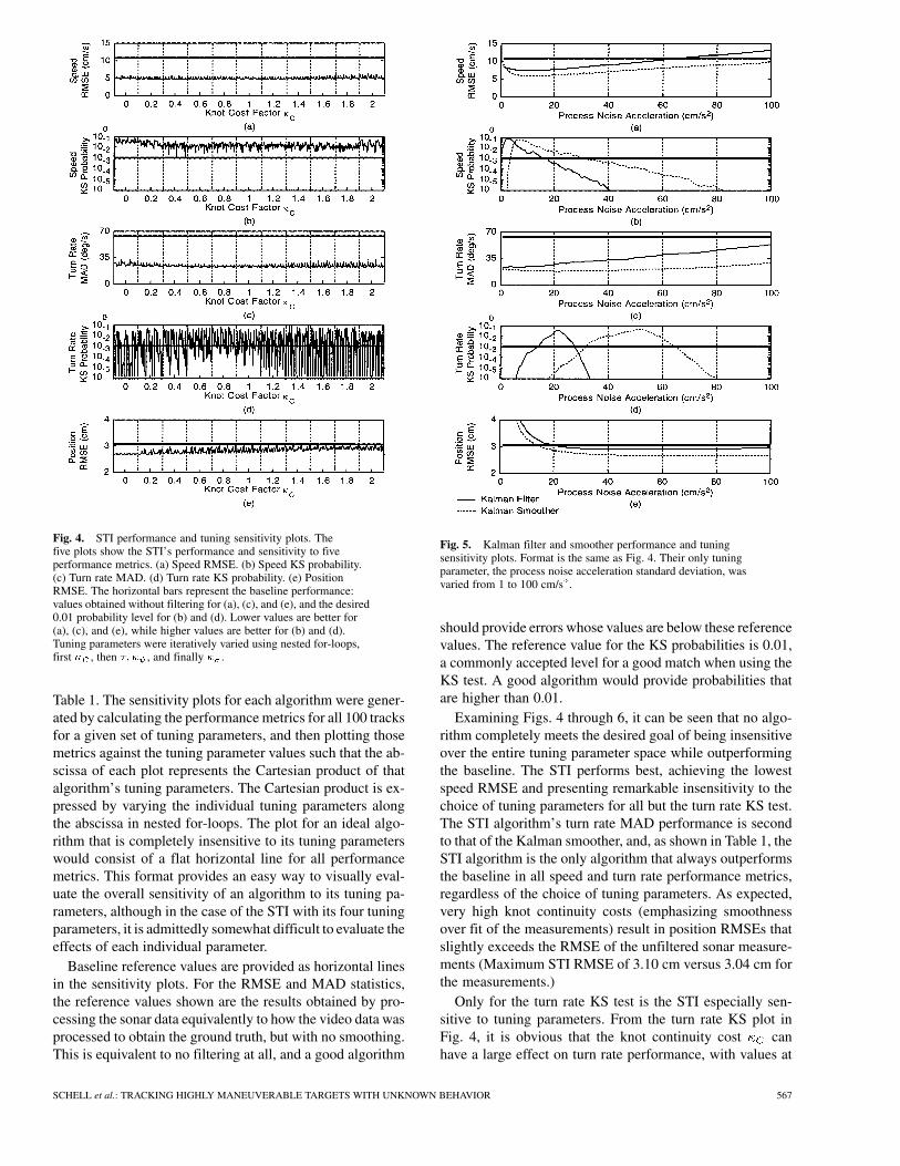
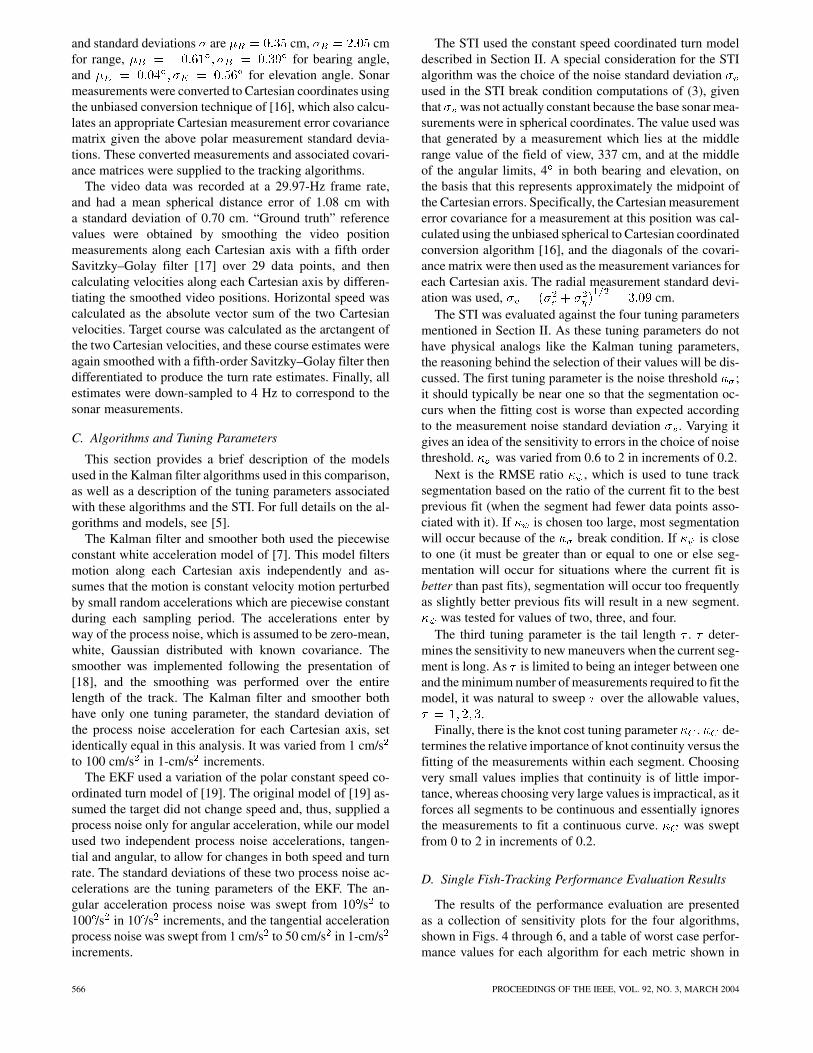
Fig. 4. STI performance and tuning sensitivity plots. Thefive plots show the STI’s performance and sensitivity to fiveperformance metrics. (a) Speed RMSE. (b) Speed KS probability.(c) Turn rate MAD. (d) Turn rate KS probability. (e) PositionRMSE. The horizontal bars represent the baseline performance:values obtained without filtering for (a), (c), and (e), and the desired0.01 probability level for (b) and (d). Lower values are better for(a), (c), and (e), while higher values are better for (b) and (d).Tuning parameters were iteratively varied using nested for-loops,first � , then �; � , and finally � .

Table 1. The sensitivity plots for each algorithm were gener-ated by calculating the performance metrics for all 100 tracksfor a given set of tuning parameters, and then plotting thosemetrics against the tuning parameter values such that the ab-scissa of each plot represents the Cartesian product of thatalgorithm’s tuning parameters. The Cartesian product is ex-pressed by varying the individual tuning parameters alongthe abscissa in nested for-loops. The plot for an ideal algo-rithm that is completely insensitive to its tuning parameterswould consist of a flat horizontal line for all performancemetrics. This format provides an easy way to visually eval-uate the overall sensitivity of an algorithm to its tuning pa-rameters, although in the case of the STI with its four tuningparameters, it is admittedly somewhat difficult to evaluate theeffects of each individual parameter.

Baseline reference values are provided as horizontal linesin the sensitivity plots. For the RMSE and MAD statistics,the reference values shown are the results obtained by pro-cessing the sonar data equivalently to how the video data wasprocessed to obtain the ground truth, but with no smoothing.This is equivalent to no filtering at all, and a good algorithm

Fig. 5. Kalman filter and smoother performance and tuningsensitivity plots. Format is the same as Fig. 4. Their only tuningparameter, the process noise acceleration standard deviation, wasvaried from 1 to 100 cm/s .

should provide errors whose values are below these referencevalues. The reference value for the KS probabilities is 0.01,a commonly accepted level for a good match when using theKS test. A good algorithm would provide probabilities thatare higher than 0.01.

Examining Figs. 4 through 6, it can be seen that no algo-rithm completely meets the desired goal of being insensitiveover the entire tuning parameter space while outperformingthe baseline. The STI performs best, achieving the lowestspeed RMSE and presenting remarkable insensitivity to thechoice of tuning parameters for all but the turn rate KS test.The STI algorithm’s turn rate MAD performance is secondto that of the Kalman smoother, and, as shown in Table 1, theSTI algorithm is the only algorithm that always outperformsthe baseline in all speed and turn rate performance metrics,regardless of the choice of tuning parameters. As expected,very high knot continuity costs (emphasizing smoothnessover fit of the measurements) result in position RMSEs thatslightly exceeds the RMSE of the unfiltered sonar measure-ments (Maximum STI RMSE of 3.10 cm versus 3.04 cm forthe measurements.)

Only for the turn rate KS test is the STI especially sen-sitive to tuning parameters. From the turn rate KS plot inFig. 4, it is obvious that the knot continuity cost canhave a large effect on turn rate performance, with values at


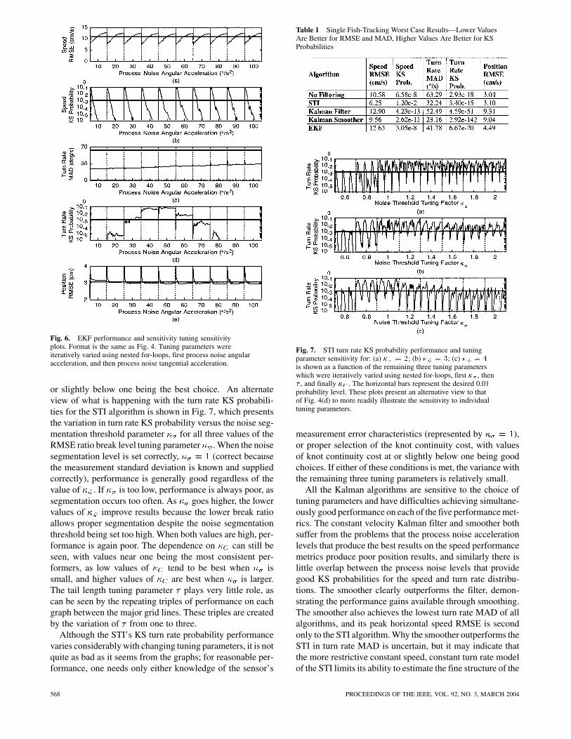
Fig. 6. EKF performance and sensitivity tuning sensitivityplots. Format is the same as Fig. 4. Tuning parameters wereiteratively varied using nested for-loops, first process noise angularacceleration, and then process noise tangential acceleration.

or slightly below one being the best choice. An alternateview of what is happening with the turn rate KS probabili-ties for the STI algorithm is shown in Fig. 7, which presentsthe variation in turn rate KS probability versus the noise seg-mentation threshold parameter for all three values of theRMSE ratio break level tuning parameter . When the noisesegmentation level is set correctly, (correct becausethe measurement standard deviation is known and suppliedcorrectly), performance is generally good regardless of thevalue of . If is too low, performance is always poor, assegmentation occurs too often. As goes higher, the lowervalues of improve results because the lower break ratioallows proper segmentation despite the noise segmentationthreshold being set too high. When both values are high, per-formance is again poor. The dependence on can still beseen, with values near one being the most consistent per-formers, as low values of tend to be best when issmall, and higher values of are best when is larger.The tail length tuning parameter plays very little role, ascan be seen by the repeating triples of performance on eachgraph between the major grid lines. These triples are createdby the variation of from one to three.

Although the STI’s KS turn rate probability performancevaries considerably with changing tuning parameters, it is notquite as bad as it seems from the graphs; for reasonable per-formance, one needs only either knowledge of the sensor’s

Table 1 Single Fish-Tracking Worst Case Results—Lower ValuesAre Better for RMSE and MAD, Higher Values Are Better for KSProbabilities

Fig. 7. STI turn rate KS probability performance and tuningparameter sensitivity for: (a) � = 2; (b) � = 3; (c) � = 4

is shown as a function of the remaining three tuning parameterswhich were iteratively varied using nested for-loops, first � , then� , and finally � . The horizontal bars represent the desired 0.01probability level. These plots present an alternative view to thatof Fig. 4(d) to more readily illustrate the sensitivity to individualtuning parameters.

measurement error characteristics (represented by ),or proper selection of the knot continuity cost, with valuesof knot continuity cost at or slightly below one being goodchoices. If either of these conditions is met, the variance withthe remaining three tuning parameters is relatively small.

All the Kalman algorithms are sensitive to the choice oftuning parameters and have difficulties achieving simultane-ously good performance on each of the five performance met-rics. The constant velocity Kalman filter and smoother bothsuffer from the problems that the process noise accelerationlevels that produce the best results on the speed performancemetrics produce poor position results, and similarly there islittle overlap between the process noise levels that providegood KS probabilities for the speed and turn rate distribu-tions. The smoother clearly outperforms the filter, demon-strating the performance gains available through smoothing.The smoother also achieves the lowest turn rate MAD of allalgorithms, and its peak horizontal speed RMSE is secondonly to the STI algorithm. Why the smoother outperforms theSTI in turn rate MAD is uncertain, but it may indicate thatthe more restrictive constant speed, constant turn rate modelof the STI limits its ability to estimate the fine structure of the


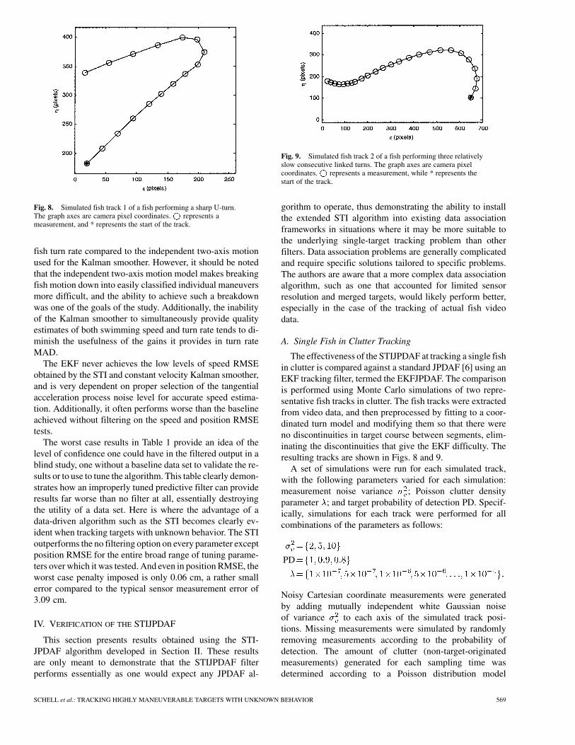
Fig. 8. Simulated fish track 1 of a fish performing a sharp U-turn.The graph axes are camera pixel coordinates. represents ameasurement, and * represents the start of the track.

fish turn rate compared to the independent two-axis motionused for the Kalman smoother. However, it should be notedthat the independent two-axis motion model makes breakingfish motion down into easily classified individual maneuversmore difficult, and the ability to achieve such a breakdownwas one of the goals of the study. Additionally, the inabilityof the Kalman smoother to simultaneously provide qualityestimates of both swimming speed and turn rate tends to di-minish the usefulness of the gains it provides in turn rateMAD.

The EKF never achieves the low levels of speed RMSEobtained by the STI and constant velocity Kalman smoother,and is very dependent on proper selection of the tangentialacceleration process noise level for accurate speed estima-tion. Additionally, it often performs worse than the baselineachieved without filtering on the speed and position RMSEtests.

The worst case results in Table 1 provide an idea of thelevel of confidence one could have in the filtered output in ablind study, one without a baseline data set to validate the re-sults or to use to tune the algorithm. This table clearly demon-strates how an improperly tuned predictive filter can provideresults far worse than no filter at all, essentially destroyingthe utility of a data set. Here is where the advantage of adata-driven algorithm such as the STI becomes clearly ev-ident when tracking targets with unknown behavior. The STIoutperforms the no filtering option on every parameter exceptposition RMSE for the entire broad range of tuning parame-ters over which it was tested. And even in position RMSE, theworst case penalty imposed is only 0.06 cm, a rather smallerror compared to the typical sensor measurement error of3.09 cm.

IV. VERIFICATION OF THE STIJPDAF

This section presents results obtained using the STI-JPDAF algorithm developed in Section II. These resultsare only meant to demonstrate that the STIJPDAF filterperforms essentially as one would expect any JPDAF al-

Fig. 9. Simulated fish track 2 of a fish performing three relativelyslow consecutive linked turns. The graph axes are camera pixelcoordinates. represents a measurement, while * represents thestart of the track.

gorithm to operate, thus demonstrating the ability to installthe extended STI algorithm into existing data associationframeworks in situations where it may be more suitable tothe underlying single-target tracking problem than otherfilters. Data association problems are generally complicatedand require specific solutions tailored to specific problems.The authors are aware that a more complex data associationalgorithm, such as one that accounted for limited sensorresolution and merged targets, would likely perform better,especially in the case of the tracking of actual fish videodata.

A. Single Fish in Clutter Tracking

The effectiveness of the STIJPDAF at tracking a single fishin clutter is compared against a standard JPDAF [6] using anEKF tracking filter, termed the EKFJPDAF. The comparisonis performed using Monte Carlo simulations of two repre-sentative fish tracks in clutter. The fish tracks were extractedfrom video data, and then preprocessed by fitting to a coor-dinated turn model and modifying them so that there wereno discontinuities in target course between segments, elim-inating the discontinuities that give the EKF difficulty. Theresulting tracks are shown in Figs. 8 and 9.

A set of simulations were run for each simulated track,with the following parameters varied for each simulation:measurement noise variance ; Poisson clutter densityparameter ; and target probability of detection PD. Specif-ically, simulations for each track were performed for allcombinations of the parameters as follows:

PD

Noisy Cartesian coordinate measurements were generatedby adding mutually independent white Gaussian noiseof variance to each axis of the simulated track posi-tions. Missing measurements were simulated by randomlyremoving measurements according to the probability ofdetection. The amount of clutter (non-target-originatedmeasurements) generated for each sampling time wasdetermined according to a Poisson distribution model


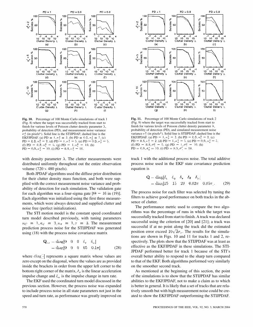
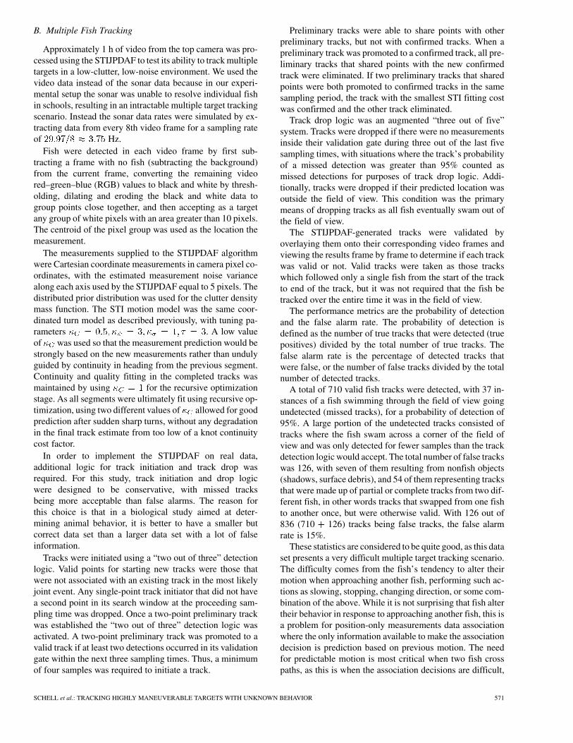
Fig. 10. Percentage of 100 Monte Carlo simulations of track 1(Fig. 8) where the target was successfully tracked from start tofinish for various levels of Poisson clutter density parameter �,probability of detection (PD), and measurement noise variance� (in pixels ). Solid line is the STIJPDAF; dashed line is theEKFJPDAF. (a) PD = 1; � = 2. (b) PD = 0:9; � = 2. (c)PD = 0:8; � = 2. (d) PD = 1; � = 5. (e) PD = 0:9; � = 5.(f) PD = 0:8; � = 5. (g) PD = 1; � = 10. (h)PD = 0:9; � = 10. (i) PD = 0:8; � = 10.

with density parameter . The clutter measurements weredistributed uniformly throughout out the entire observationvolume (720 480 pixels).

Both JPDAF algorithms used the diffuse prior distributionfor their clutter density mass function, and both were sup-plied with the correct measurement noise variance and prob-ability of detection for each simulation. The validation gatefor each algorithm was a four-sigma gate [ in (19)].Each algorithm was initialized using the first three measure-ments, which were always detected and supplied clutter andnoise free (perfect initialization).

The STI motion model is the constant speed coordinatedturn model described previously, with tuning parameters

. The measurementprediction process noise for the STIJPDAF was generatedusing (18) with the process noise covariance matrix

(28)

where represents a square matrix whose values arezero except on the diagonal, where the values are as providedinside the brackets in order from the upper left corner to thebottom right corner of the matrix, is the linear accelerationimpulse change and is the impulse change in turn rate.

The EKF used the coordinated turn model discussed in theprevious section. However, the process noise was expandedto include process noise in all state parameters not just in thespeed and turn rate, as performance was greatly improved on

Fig. 11. Percentage of 100 Monte Carlo simulations of track 2(Fig. 9) where the target was successfully tracked from start tofinish for various levels of Poisson clutter density parameter �,probability of detection (PD), and simulated measurement noisevariance � (in pixels ). Solid line is STIJPDAF; dashed line is theEKFJPDAF. (a) PD = 1; � = 2. (b) PD = 0:9; � = 2. (c)PD = 0:8; � = 2. (d) PD = 1; � = 5. (e) PD = 0:9; � = 5.(f) PD = 0:8; � = 5. (g) PD = 1; � = 10. (h)PD = 0:9; � = 10. (i) PD = 0:8; � = 10.

track 1 with the additional process noise. The total additiveprocess noise used in the EKF state covariance predictionequation is

(29)

The process noise for each filter was selected by tuning thefilters to achieve good performance on both tracks in the ab-sence of clutter.

The performance metric used to compare the two algo-rithms was the percentage of runs in which the target wassuccessfully tracked from start to finish. A track was declaredsuccessful using the criterion of [20] and [21]; a track wassuccessful if at no point along the track did the estimatedposition error exceed . The results for the simula-tions are shown in Figs. 10 and 11 for tracks 1 and 2, re-spectively. The plots show that the STIJPDAF was at least aseffective as the EKFJPDAF in these simulations. The STI-JPDAF performed better for track 1 because of the STI’soverall better ability to respond to the sharp turn comparedto that of the EKF. Both algorithms performed very similarlyon the smoother second track.

As mentioned at the beginning of this section, the pointof the simulations is to show that the STIJPDAF has similarabilities to the EKFJPDAF, not to make a claim as to whichis better in general. It is likely that a set of tracks that are rela-tively smooth but with high measurement noise could be cre-ated to show the EKFJPDAF outperforming the STIJPDAF.


B. Multiple Fish Tracking

Approximately 1 h of video from the top camera was pro-cessed using the STIJPDAF to test its ability to track multipletargets in a low-clutter, low-noise environment. We used thevideo data instead of the sonar data because in our experi-mental setup the sonar was unable to resolve individual fishin schools, resulting in an intractable multiple target trackingscenario. Instead the sonar data rates were simulated by ex-tracting data from every 8th video frame for a sampling rateof Hz.

Fish were detected in each video frame by first sub-tracting a frame with no fish (subtracting the background)from the current frame, converting the remaining videored–green–blue (RGB) values to black and white by thresh-olding, dilating and eroding the black and white data togroup points close together, and then accepting as a targetany group of white pixels with an area greater than 10 pixels.The centroid of the pixel group was used as the location themeasurement.

The measurements supplied to the STIJPDAF algorithmwere Cartesian coordinate measurements in camera pixel co-ordinates, with the estimated measurement noise variancealong each axis used by the STIJPDAF equal to 5 pixels. Thedistributed prior distribution was used for the clutter densitymass function. The STI motion model was the same coor-dinated turn model as described previously, with tuning pa-rameters . A low valueof was used so that the measurement prediction would bestrongly based on the new measurements rather than undulyguided by continuity in heading from the previous segment.Continuity and quality fitting in the completed tracks wasmaintained by using for the recursive optimizationstage. As all segments were ultimately fit using recursive op-timization, using two different values of allowed for goodprediction after sudden sharp turns, without any degradationin the final track estimate from too low of a knot continuitycost factor.

In order to implement the STIJPDAF on real data,additional logic for track initiation and track drop wasrequired. For this study, track initiation and drop logicwere designed to be conservative, with missed tracksbeing more acceptable than false alarms. The reason forthis choice is that in a biological study aimed at deter-mining animal behavior, it is better to have a smaller butcorrect data set than a larger data set with a lot of falseinformation.

Tracks were initiated using a “two out of three” detectionlogic. Valid points for starting new tracks were those thatwere not associated with an existing track in the most likelyjoint event. Any single-point track initiator that did not havea second point in its search window at the proceeding sam-pling time was dropped. Once a two-point preliminary trackwas established the “two out of three” detection logic wasactivated. A two-point preliminary track was promoted to avalid track if at least two detections occurred in its validationgate within the next three sampling times. Thus, a minimumof four samples was required to initiate a track.

Preliminary tracks were able to share points with otherpreliminary tracks, but not with confirmed tracks. When apreliminary track was promoted to a confirmed track, all pre-liminary tracks that shared points with the new confirmedtrack were eliminated. If two preliminary tracks that sharedpoints were both promoted to confirmed tracks in the samesampling period, the track with the smallest STI fitting costwas confirmed and the other track eliminated.

Track drop logic was an augmented “three out of five”system. Tracks were dropped if there were no measurementsinside their validation gate during three out of the last fivesampling times, with situations where the track’s probabilityof a missed detection was greater than 95% counted asmissed detections for purposes of track drop logic. Addi-tionally, tracks were dropped if their predicted location wasoutside the field of view. This condition was the primarymeans of dropping tracks as all fish eventually swam out ofthe field of view.

The STIJPDAF-generated tracks were validated byoverlaying them onto their corresponding video frames andviewing the results frame by frame to determine if each trackwas valid or not. Valid tracks were taken as those trackswhich followed only a single fish from the start of the trackto end of the track, but it was not required that the fish betracked over the entire time it was in the field of view.

The performance metrics are the probability of detectionand the false alarm rate. The probability of detection isdefined as the number of true tracks that were detected (truepositives) divided by the total number of true tracks. Thefalse alarm rate is the percentage of detected tracks thatwere false, or the number of false tracks divided by the totalnumber of detected tracks.

A total of 710 valid fish tracks were detected, with 37 in-stances of a fish swimming through the field of view goingundetected (missed tracks), for a probability of detection of95%. A large portion of the undetected tracks consisted oftracks where the fish swam across a corner of the field ofview and was only detected for fewer samples than the trackdetection logic would accept. The total number of false trackswas 126, with seven of them resulting from nonfish objects(shadows, surface debris), and 54 of them representing tracksthat were made up of partial or complete tracks from two dif-ferent fish, in other words tracks that swapped from one fishto another once, but were otherwise valid. With 126 out of836 (710 126) tracks being false tracks, the false alarmrate is 15%.

These statistics are considered to be quite good, as this dataset presents a very difficult multiple target tracking scenario.The difficulty comes from the fish’s tendency to alter theirmotion when approaching another fish, performing such ac-tions as slowing, stopping, changing direction, or some com-bination of the above. While it is not surprising that fish altertheir behavior in response to approaching another fish, this isa problem for position-only measurements data associationwhere the only information available to make the associationdecision is prediction based on previous motion. The needfor predictable motion is most critical when two fish crosspaths, as this is when the association decisions are difficult,


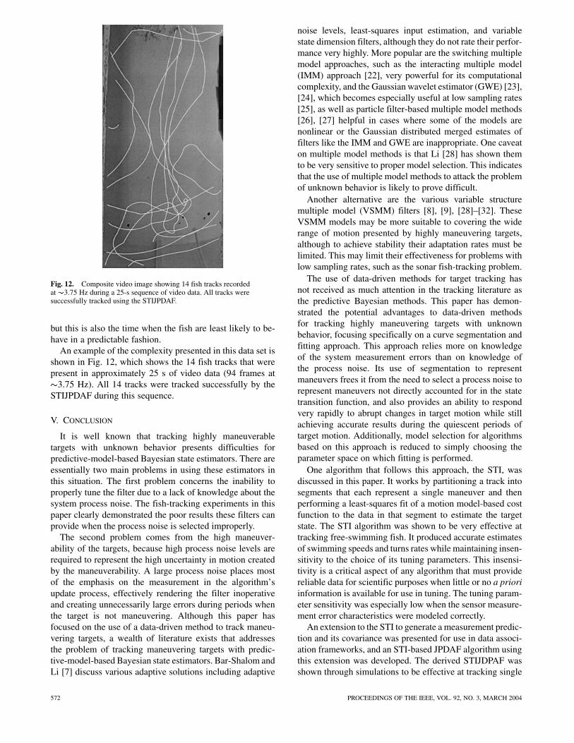
Fig. 12. Composite video image showing 14 fish tracks recordedat �3.75 Hz during a 25-s sequence of video data. All tracks weresuccessfully tracked using the STIJPDAF.

but this is also the time when the fish are least likely to be-have in a predictable fashion.

An example of the complexity presented in this data set isshown in Fig. 12, which shows the 14 fish tracks that werepresent in approximately 25 s of video data (94 frames at

3.75 Hz). All 14 tracks were tracked successfully by theSTIJPDAF during this sequence.

V. CONCLUSION

It is well known that tracking highly maneuverabletargets with unknown behavior presents difficulties forpredictive-model-based Bayesian state estimators. There areessentially two main problems in using these estimators inthis situation. The first problem concerns the inability toproperly tune the filter due to a lack of knowledge about thesystem process noise. The fish-tracking experiments in thispaper clearly demonstrated the poor results these filters canprovide when the process noise is selected improperly.

The second problem comes from the high maneuver-ability of the targets, because high process noise levels arerequired to represent the high uncertainty in motion createdby the maneuverability. A large process noise places mostof the emphasis on the measurement in the algorithm’supdate process, effectively rendering the filter inoperativeand creating unnecessarily large errors during periods whenthe target is not maneuvering. Although this paper hasfocused on the use of a data-driven method to track maneu-vering targets, a wealth of literature exists that addressesthe problem of tracking maneuvering targets with predic-tive-model-based Bayesian state estimators. Bar-Shalom andLi [7] discuss various adaptive solutions including adaptive

noise levels, least-squares input estimation, and variablestate dimension filters, although they do not rate their perfor-mance very highly. More popular are the switching multiplemodel approaches, such as the interacting multiple model(IMM) approach [22], very powerful for its computationalcomplexity, and the Gaussian wavelet estimator (GWE) [23],[24], which becomes especially useful at low sampling rates[25], as well as particle filter-based multiple model methods[26], [27] helpful in cases where some of the models arenonlinear or the Gaussian distributed merged estimates offilters like the IMM and GWE are inappropriate. One caveaton multiple model methods is that Li [28] has shown themto be very sensitive to proper model selection. This indicatesthat the use of multiple model methods to attack the problemof unknown behavior is likely to prove difficult.

Another alternative are the various variable structuremultiple model (VSMM) filters [8], [9], [28]–[32]. TheseVSMM models may be more suitable to covering the widerange of motion presented by highly maneuvering targets,although to achieve stability their adaptation rates must belimited. This may limit their effectiveness for problems withlow sampling rates, such as the sonar fish-tracking problem.

The use of data-driven methods for target tracking hasnot received as much attention in the tracking literature asthe predictive Bayesian methods. This paper has demon-strated the potential advantages to data-driven methodsfor tracking highly maneuvering targets with unknownbehavior, focusing specifically on a curve segmentation andfitting approach. This approach relies more on knowledgeof the system measurement errors than on knowledge ofthe process noise. Its use of segmentation to representmaneuvers frees it from the need to select a process noise torepresent maneuvers not directly accounted for in the statetransition function, and also provides an ability to respondvery rapidly to abrupt changes in target motion while stillachieving accurate results during the quiescent periods oftarget motion. Additionally, model selection for algorithmsbased on this approach is reduced to simply choosing theparameter space on which fitting is performed.

One algorithm that follows this approach, the STI, wasdiscussed in this paper. It works by partitioning a track intosegments that each represent a single maneuver and thenperforming a least-squares fit of a motion model-based costfunction to the data in that segment to estimate the targetstate. The STI algorithm was shown to be very effective attracking free-swimming fish. It produced accurate estimatesof swimming speeds and turns rates while maintaining insen-sitivity to the choice of its tuning parameters. This insensi-tivity is a critical aspect of any algorithm that must providereliable data for scientific purposes when little or no a prioriinformation is available for use in tuning. The tuning param-eter sensitivity was especially low when the sensor measure-ment error characteristics were modeled correctly.

An extension to the STI to generate a measurement predic-tion and its covariance was presented for use in data associ-ation frameworks, and an STI-based JPDAF algorithm usingthis extension was developed. The derived STIJDPAF wasshown through simulations to be effective at tracking single


fish in clutter and through the use of real-world video data tobe effective at tracking multiple free-swimming fish.

ACKNOWLEDGMENT

C. Schell would like to thank his thesis adviser J. S. Jaffefor providing support and lab resources to perform the fish-tracking experiment described in this paper.

REFERENCES

[1] S. P. Linder, M. D. Ryan, and R. J. Quintin, “Concise track char-acterization of maneuvering targets,” presented at the AIAA Conf.Guidance, Navigation, and Control, Montreal, QB, Canada, 2001.

[2] P. L. Rosin and G. A. W. West, “Segmenting curves into elliptic arcsand straight lines,” in Proc. 3rd Int. Conf. Computer Vision, 1990,pp. 75–78.

[3] S. Hsin-Teng and H. Wu-Chih, “Multiprimitive segmentation ofplanar curves-a two-level breakpoint classification and tuningapproach,” IEEE Trans. Pattern Anal. Machine Intell., vol. 21, pp.791–797, Aug. 1999.

[4] L. Wenyin and D. Dori, “Incremental arc segmentation algorithmand its evaluation,” IEEE Trans. Pattern Anal. Machine Intell., vol.20, pp. 424–431, Apr. 1998.

[5] C. Schell, “Advanced tracking algorithms for the study of fine scalefish behavior,” Ph.D. dissertation, Univ. California, San Diego, 2003.

[6] Y. Bar-Shalom and X. R. Li, Multitarget-Multisensor Tracking:Principles and Techniques. Storrs, CT: YBS, 1995.

[7] , Estimation and Tracking: Principles Techniques, and Soft-ware. Storrs, CT: YBS, 1998.

[8] V. P. Jilkov, D. S. Angelova, and T. A. Semerdjiev, “Design andcomparison of mode-set adaptive IMM algorithms for maneuveringtarget tracking,” IEEE Trans. Aerosp. Electron. Syst., vol. 35, pp.343–350, Jan. 1999.

[9] E. Semerdjiev, L. Mihaylova, and X. R. Li, “Variable- andfixed-structure augmented IMM algorithms using coordinated turnmodel,” in Proc. 3rd Int. Conf. Information Fusion, vol. 1, 2000,pp. 25–32.

[10] J. R. Brett and T. D. D. Groves, “Physiological energetics,” in FishPhysiology. New York: Academic, 1979, vol. 8, pp. 279–352.

[11] P. W. Webb, “Hydrodynamics and energetics of fish propulsion,”Bull. Fisheries Res. Board Canada, vol. 190, pp. 1–158, 1975.

[12] M. Tang, D. Boisclair, C. Menard, and J. A. Downing, “Influence ofbody weight, swimming characteristics, and water temperature onthe cost of swimming in brook trout (Salvelinus fontinalis),” Cana-dian J. Fisheries Aquatic Sci., vol. 57, pp. 1482–1488, July 2000.

[13] P. W. Webb, “Composition and mechanics of routine swimmingof rainbow trout oncorhynchus-mykiss,” Canadian J. FisheriesAquatic Sci., vol. 48, pp. 583–590, 1991.

[14] D. Boisclair and M. Tang, “Empirical analysis of the influence ofswimming pattern on the net energetic cost of swimming in fishes,”J. Fish Biol., vol. 42, pp. 169–183, 1993.

[15] D. G. Harper and R. W. Blake, “A critical analysis of the use ofhigh-speed film to determine maximum accelerations of fish,” J.Exp. Biol., vol. 142, pp. 465–472, 1989.

[16] L. Mo, X. Song, Y. Zhou, K. Sun Zhong, and Y. Bar-Shalom, “Un-biased converted measurements for tracking,” IEEE Trans. Aerosp.Electron. Syst., vol. 34, pp. 1023–1027, July 1998.

[17] W. H. Press, S. A. Teukolsky, W. T. Vetterling, and B. P. Flannery,Numerical Recipes in C, The Art of Scientific Computing, 2nded. New York: Press Syndicate Univ. Cambridge, 1996.

[18] S. Roweis and Z. Ghahramani, “A unifying review of linear gaussianmodels,” Neural Comput., vol. 11, pp. 305–345, Feb. 1999.

[19] F. Gustafsson and A. J. Isaksson, “Best choice of coordinate systemfor tracking coordinated turns,” in Proc. 35th IEEE Conf. Decisionand Control, vol. 3, 1996, pp. 3145–3150.

[20] S. R. Rogers, “Diffusion analysis of track loss in clutter,” IEEETrans. Aerosp. Electron. Syst., vol. 27, pp. 380–387, Mar. 1991.

[21] D. Avitzour, “Stochastic simulation Bayesian approach to multi-target tracking,” in IEE Proc. F, Radar, Sonar Navigat., vol. 142,Apr. 1995, pp. 41–44.

[22] H. A. P. Blom and Y. Bar-Shalom, “The interacting multiple modelalgorithm for systems with Markovian switching coefficients,” IEEETrans. Automat. Contr., vol. 33, pp. 780–783, Aug. 1988.

[23] D. D. Sworder, J. E. Boyd, R. J. Eliott, and R. G. Hutchins, “Datafusion using multiple models,” in Conf. Rec. 34th Asilomar Conf.Signals, Systems and Computers, vol. 2, 2000, pp. 1749–1753.

[24] C. T. Leondes, D. D. Sworder, and J. E. Boyd, “Multiple modelmethods in path following,” J. Math. Anal. Appl., vol. 251, pp.609–623, Nov. 15, 2000.

[25] D. D. Sworder and J. E. Boyd, “Measurement rate reduction in hy-brid systems,” J. Guidance Control Dynamics, vol. 24, pp. 411–414,Mar.–Apr. 2001.

[26] R. Karlsson and N. Bergman, “Auxiliary particle filters for trackinga maneuvering target,” in Proc. 39th IEEE Conf. Decision and Con-trol, vol. 4, 2000, pp. 3891–3895.

[27] A. Doucet, N. J. Gordon, and V. Krishnamurthy, “Sequential sim-ulation-based estimation of jump Markov linear systems,” in Proc.39th IEEE Conf. Decision and Control, 2000, pp. 1166–1171.

[28] X. R. Li and Y. Bar-Shalom, “Multiple-model estimation with vari-able structure,” IEEE Trans. Automat. Contr., vol. 41, pp. 478–493,Apr. 1996.

[29] X. R. Li, Z. Xiaorong, and Z. Youmin, “Multiple-model estima-tion with variable structure. III. Model-group switching algorithm,”IEEE Trans. Aerosp. Electron. Syst., vol. 35, pp. 225–241, Jan. 1999.

[30] X. R. Li and Z. Youmin, “Multiple-model estimation with variablestructure. V. Likely-model set algorithm,” IEEE Trans. Aerosp. Elec-tron. Syst., vol. 36, pp. 448–466, Apr. 2000.

[31] X. R. Li, Z. Youmin, and Z. Xiaorong, “Multiple-model estimationwith variable structure. IV. Design and evaluation of model-groupswitching algorithm,” IEEE Trans. Aerosp. Electron. Syst., vol. 35,pp. 242–254, Jan. 1999.

[32] X. R. Li, “Multiple-model estimation with variable structure. II.Model-set adaptation,” IEEE Trans. Automatic Control, vol. 45, pp.2047–2060, Nov. 2000.

Chad Schell (Member, IEEE) received the B.S.degree in electrical engineering from the Uni-versity of New Mexico, Albuquerque, in 1996,and the M.S. and Ph.D. degrees in electricalengineering (applied ocean science) from theUniversity of California, San Diego, La Jolla, in2000 and 2003 respectively.

From 1991 to 1996, he worked at Sandia Na-tional Laboratories in the Intelligent Systems andRobotics and the Microsensors divisions. He cur-rently conducts research on geolocation systems

at Rincon Research Corporation in Tucson, AZ, and operates his own con-sumer electronics business.

Dr. Schell received a National Science Foundation fellowship.

Stephen Paul Linder received the B.S. degree inmechanical engineering from the MassachusettsInstitute of Technology, Cambridge, in 1982 andthe M.S. degree in computer systems engineeringand the Ph.D. degree in electrical and computersystems engineering from Northeastern Univer-sity, Boston, MA, in 1996 and 1998, respectively.

He was with the Applied Research Laboratory,Pennsylvania State University, University Park,working on target tracking and sensor data fu-sion, and a Faculty Member in computer science

at the State University of New York, Plattsburgh. He is currently in theComputer Science Department, Dartmouth College, Hanover, NH, and isworking on projects that include the track prediction of bouncing ball usinglimited data rate cameras, tracking of cell phones using antenna arrays, anddynamic health assessment of first responders. He also teaches classes inmountaineering or sea kayaking when not sitting in front of the computer.See http://alum.mit.edu/www/spl for more details.


James R. Zeidler (Fellow, IEEE) received thePh.D. degree in physics from the University ofNebraska, Lincoln, in 1972. From 1974 to 2003,he was a Scientist at the Space and Naval WarfareSystems Center, San Diego, CA, and from 1988to 2003, he was an Adjunct Professor of Electricaland Computer Engineering (ECE) Department atthe University of California, San Diego (UCSD).He is currently a Senior Research Scientist/SeniorLecturer in the ECE department at UCSD and afaculty member of the Center for Wireless Com-

munications at UCSD and of the California Institute for Telecommunica-tions and Information Technology at UCSD and the University of California,Irvine. He has written more than 200 technical publications and holds 12U.S. patents.

Dr, Zeidler received the IEEE Frederick Ellersick best paper award at the1995 IEEE Military Communications Conference, the Lauritsen-Bennetaward for achievement in science in 2000, and the Navy MeritoriousCivilian Service Award in 1991. He was an Associate Editor of the IEEETRANSACTIONS ON SIGNAL PROCESSING from 1991 to 1994.
