225EMPIRICAL

MACRO-ECONOMICMODEL OF

THE FINNISHECONOMY

(EMMA)

Markku Lehmus

PALKANSAAJIEN TUTKIMUSLAITOS •TYÖPAPEREITA LABOUR INSTITUTE FOR ECONOMIC RESEARCH • DISCUSSION PAPERS

* This study has been funded by Palkansaajasäätiö.

I am grateful to Eero Lehto and Matti Virén for help in constructing the model and preparing this report.

** Markku Lehmus, Labour Institute for Economic Research,

Pitkänsillanranta 3 A, 00530 Helsinki, Finland, markku.lehmus@labour.fi.

Helsinki 2007

225

Empirical Macroeconomic Model of the Finnish Economy(EMMA)*

Markku Lehmus**

ISBN 978−952−209−034−8 ISSN 1795−1801

Abstract

This paper provides a review of the empirical macroeconomic model (EMMA) built for forecasting

purposes at the Finnish Labour Institute for Economic Research. The model is quite small,

consisting of 71 endogenous and 70 exogenous variables. The number of behavioural equations is

15. The basis of the model is Keynesian, although the model has some novel properties. They are

the treatment of the supply side and prices that follow the routes of the neoclassical synthesis. The

parameters of the model are estimated from quarterly data that cover the years 1990-2005. The

model also contains a Kalman-filtered variable to control the deep recession in Finland at the

beginning of the ’90s. This special feature brings the model closer to the new calibrated models.

1. Motivation

Earlier, it was considered self-evident that most macroeconomic variables can be forecasted

relatively accurately if the forecasters have the necessary data and proper models. Thus, investing in

forecasting would pay off. Hence, for instance, the development of larger and more complicated

models would be useful. After the rational expectations revolution in the 1970s things are no longer

that simple. We have learned that in many cases random walk forecast cannot be beaten by

structural models and other sort of forecasting techniques. That is because variables which are

contingent on wealth variables basically depend on current expectations of the future path of prices.

Thus, if we want to beat the random walk forecast (a forecast where the current value is used as the

best proxy for the next period's value) we ought to know how expectations will change. That sounds

impossible. Even if this is the case with certain variables, it is not, however, true with all. In many

cases there are various market frictions which can be exploited in forecasting. Thus, prices and

wages may be sticky, adjustment cost may dictate the path of adjustment with volume variables

and, finally, the forecasters may have some information advantage compared with the general

public.

Against this background it seems self-evident that the quality of forecasts can be improved by

using more resources in the forecasting process. This is true with the development of models, in

particular. Models automatically impose some necessary adding-up and homogeneity restrictions

which make the forecast logically consistent. Moreover, models also allow comparison of

alternative time-paths of exogenous variables and policy rules. Finally, models provide meaningful

estimates of uncertainty which is related to future time paths of different variables. Without a proper

2

model these necessary steps cannot be taken and forecasting looks like guessing the right numbers.

In this case, the outcome of forecasting process must also be limited to a few indicators, like the

GDP. Although, the media is usually only interested in (future) GDP growth rates that is not the

same as the future economic situation. Take for instance, the public sector. The growth rate of GDP

tells very little on the size of the public sector, the deficit and debt ratios, and the structure of

taxation and expenditures. Obviously these numbers can be forecasted (guessed?) separately but

there is absolutely no guarantee that the outcomes correspond to any internally consistent set of

values.

One may outline these causalities in one’s own head, but in practice the most sensible thing to do

is to formulate a model that includes the essential dependences. This kind of simultaneous

economic models has been generally used throughout the western world since the days of Jan

Tinbergen (1939), the pioneer of macroeconomic model building. Nevertheless, forecasting and

policy analysis with macro models is poorly rooted in the Finnish culture. Only the Bank of Finland

has continually used and cultivated its macro models. In the other research institutes the models

have played a secondary role and they have been used occasionally (in the 1970s and 1980s the

models of the Ministry of Finance's (entitled KESSU) and the Research Institute of the Finnish

Economy ought to be mentioned here). Except for the Bank of Finland, all the forecasts in Finland

are made without a formal model framework and rest, at the highest, on the standard computation

schemes of the national accounts system.

The decision of Labour Institute to build a macro economic model basically derives from an aim

to increase the analytical elements in the Institution’s forecasting process. As stated above,

modelling improves the inner consistence of a forecast and gives an opportunity to track down the

ideas behind the forecast estimates. The experienced difficulties to foresee the turning points in the

economic development are closely related to this. Without a model, the turning points are really

hard to forecast, instead, it is very common that forecasters just continue the historical path and

even mimic the forecasts made by other institutions.

In addition, the macroeconomic model can be used as a device to make various kinds of

simulations. We can then investigate, for example, the outcomes of specified policy measures. Even

the effects of a change in any exogenous variable can be examined.

3

2. The model

As has already been said, the history of macroeconomic modelling begins from the 1930s. The

traditional macro models are Keynesian. The rise of neoclassical theory and rational expectations

have made the builders of macroeconomic models improve their models. The supply side of the

economy has received more attention and there have been attempts to incorporate rational

expectations in macroeconomic models. Theoretical development has also given rise to the new

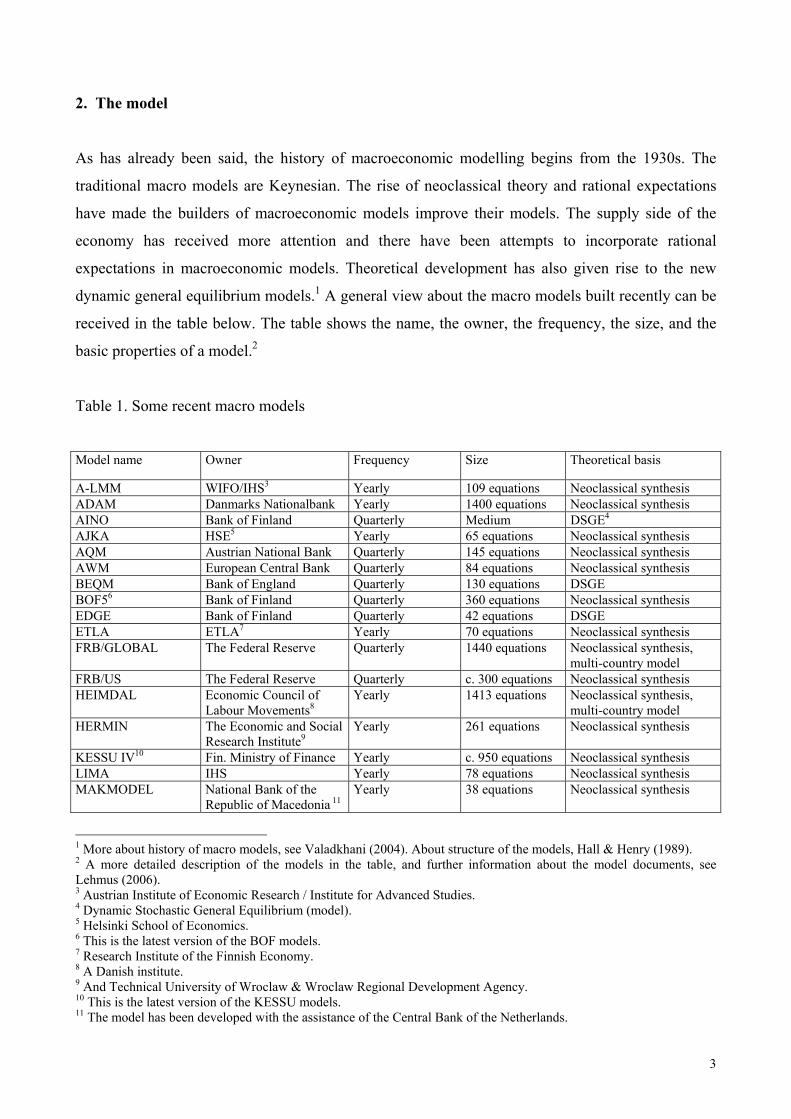
dynamic general equilibrium models.1 A general view about the macro models built recently can be

received in the table below. The table shows the name, the owner, the frequency, the size, and the

basic properties of a model.2

Table 1. Some recent macro models

Model name Owner Frequency Size Theoretical basis

A-LMM WIFO/IHS3 Yearly 109 equations Neoclassical synthesis ADAM Danmarks Nationalbank Yearly 1400 equations Neoclassical synthesis AINO Bank of Finland Quarterly Medium DSGE4 AJKA HSE5 Yearly 65 equations Neoclassical synthesis AQM Austrian National Bank Quarterly 145 equations Neoclassical synthesis AWM European Central Bank Quarterly 84 equations Neoclassical synthesis BEQM Bank of England Quarterly 130 equations DSGE BOF56 Bank of Finland Quarterly 360 equations Neoclassical synthesis EDGE Bank of Finland Quarterly 42 equations DSGE ETLA ETLA7 Yearly 70 equations Neoclassical synthesis FRB/GLOBAL The Federal Reserve Quarterly 1440 equations Neoclassical synthesis,

multi-country model FRB/US The Federal Reserve Quarterly c. 300 equations Neoclassical synthesis HEIMDAL Economic Council of

Labour Movements8 Yearly 1413 equations Neoclassical synthesis,

multi-country model HERMIN The Economic and Social

Research Institute9 Yearly 261 equations Neoclassical synthesis

KESSU IV10 Fin. Ministry of Finance Yearly c. 950 equations Neoclassical synthesis LIMA IHS Yearly 78 equations Neoclassical synthesis MAKMODEL National Bank of the

Republic of Macedonia 11 Yearly 38 equations Neoclassical synthesis

1 More about history of macro models, see Valadkhani (2004). About structure of the models, Hall & Henry (1989). 2 A more detailed description of the models in the table, and further information about the model documents, see Lehmus (2006). 3 Austrian Institute of Economic Research / Institute for Advanced Studies. 4 Dynamic Stochastic General Equilibrium (model). 5 Helsinki School of Economics. 6 This is the latest version of the BOF models. 7 Research Institute of the Finnish Economy. 8 A Danish institute. 9 And Technical University of Wroclaw & Wroclaw Regional Development Agency. 10 This is the latest version of the KESSU models. 11 The model has been developed with the assistance of the Central Bank of the Netherlands.

4

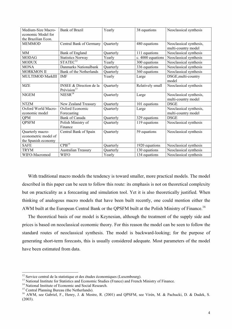
Medium-Size Macro-economic Model for the Brazilian Econ.

Bank of Brazil Yearly 38 equations Neoclassical synthesis

MEMMOD Central Bank of Germany Quarterly 480 equations Neoclassical synthesis, multi-country model

MM Bank of England Quarterly 111 equations Neoclassical synthesis MODAG Statistics Norway Yearly c. 4000 equations Neoclassical synthesis MODUX STATEC12 Yearly 300 equations Neoclassical synthesis MONA Danmarks Nationalbank Quarterly 336 equations Neoclassical synthesis MORKMON II Bank of the Netherlands Quarterly 360 equations Neoclassical synthesis MULTIMOD MarkIII IMF Yearly Large DSGE,multi-country

model MZE INSEE & Direction de la

Prévision13 Quarterly Relatively small Neoclassical synthesis

NIGEM NIESR14 Quarterly Large Neoclassical synthesis, multi-country model

NTZM New Zealand Treasury Quarterly 101 equations DSGE Oxford World Macro-economic model

Oxford Economic Forecasting

Quarterly Large Neoclassical synthesis, multi-country model

QPM Bank of Canada Quarterly 329 equations DSGE QPSFM Polish Ministry of

Finance Quarterly 119 equations Neoclassical synthesis

Quarterly macro-econometric model of the Spanish economy

Central Bank of Spain Quarterly 59 equations Neoclassical synthesis

SAFE CPB15 Quarterly 1920 equations Neoclassical synthesis TRYM Australian Treasury Quarterly 130 equations Neoclassical synthesis WIFO-Macromod WIFO Yearly 134 equations Neoclassical synthesis

With traditional macro models the tendency is toward smaller, more practical models. The model

described in this paper can be seen to follow this route: its emphasis is not on theoretical complexity

but on practicality as a forecasting and simulation tool. Yet it is also theoretically justified. When

thinking of analogous macro models that have been built recently, one could mention either the

AWM built at the European Central Bank or the QPSFM built at the Polish Ministry of Finance.16

The theoretical basis of our model is Keynesian, although the treatment of the supply side and

prices is based on neoclassical economic theory. For this reason the model can be seen to follow the

standard routes of neoclassical synthesis. The model is backward-looking; for the purpose of

generating short-term forecasts, this is usually considered adequate. Most parameters of the model

have been estimated from data.

12 Service central de la statistique et des études économiques (Luxembourg). 13 National Institute for Statistics and Economic Studies (France) and French Ministry of Finance. 14 National Institute of Economic and Social Research. 15 Central Planning Bureau (the Netherlands). 16 AWM, see Gabriel, F., Henry, J. & Mestre, R. (2001) and QPSFM, see Virén, M. & Pachucki, D. & Dudek, S. (2003).

5

The model consists of 71 endogenous and 73 exogenous variables. The number of behavioural

equations is 15. The public sector identities, in particular, enlarge the model. The nature of the

model is quite aggregated: the economy consists of the private and public sectors. The equations of

the model can be divided into four blocks: production function and factor demand equations,

aggregate demand equations, price and wage equations, and public sector identities. The production

function is modelled with the conventional Cobb-Douglas function. The model also includes the

output gap which is based on the NAIRU rate. The NAIRU rate is assumed to depend on long-term

unemployment.

The model equations are estimated with OLS (ordinary least squares). The long-run equilibrium

relationships and short-term dynamic corrections of the behavioural equations are estimated using

an error correction model (ECM) framework. From the point of view of time-series analysis, these

correspond to the two-stage Engle-Granger (1987) method.

The most demanding part in modelling the Finnish economy in the period 1990-2005 is the deep

recession in years 1991-1994. Owing to the recession, it is almost impossible to get reasonable

estimates for the coefficients of the equations. To solve this problem, we use the Kalman filter to

estimate a time-varying parameter included in the scale of the production function. This parameter

is used later on as a ”recession dummy” variable in many equations. This way the shock caused by

the recession is controlled. The solution can be regarded as an indispensable compromise to deal

with one of the deepest recessions in western countries during modern times. Other methods, for

instance the use of different dummies indicating structural change, would have probably led to

unpractical and complicated applications. This novel feature also brings this traditional model

closer to the new calibrated macro models.

The model described in this discussion paper is a beta version and will be developed further. In

the near future, we intend to concentrate on the labour market and fiscal blocks of the model. Then,

especially the relationship between labour supply and taxes (the tax wedge) is considered. The data

bank links, computation, and simulation routines will also be developed so that the practial use of

the model will be relatively easy. The paper is organized as follows. First we briefly describe the

data. Then we analyse the main structure of the four equation blocks of the model. Finally, we do

some simulations with the model.

6

3. The Data

The data of the macroeconomic model covers the years 1990-2005. The data is quarterly and is

based mainly on the national accounts of Statistics Finland. Other data sources have been the Bank

of Finland, VATT, Eurostat, and the World Bank. The two latter ones have been used to collect the

data from foreign countries. The money and interest rate series come from the Bank of Finland. The

tax rate data is based on the calculation of the Government Institute for Economic Research

(VATT). Our aim has been to use the series that are seasonally adjusted by Statistics Finland as

much as possible. In some cases only unadjusted time series exists. These series have been

seasonally adjusted with the Tramo/Seats method (which is the same method that is used in

Statistics Finland).17

In addition, some sectoral accounts are only available on a yearly basis. These series have been

disaggregated with the help of relevant reference series. This has been done with the Ecotrim

program developed in Eurostat. The model system operates in the Eviews environment but some

calculations have been done outside the actual model. This mainly concerns the public sector and

the foreign environment.18 These ”satellite calculations” are found in Excel. Chapters 5 and 7 and

Appendix 2 will illustrate the public sector and foreign sector calculations further.

4. The production function and potential output

Neoclassical theory emphasizes the role of the supply side in the economy. The supply is usually

determined by the production function. When constructing the production function, the familiar

question is: Should it be the CES or the Cobb-Douglas function? Before answering this, we start

from some presumptions.

We make an assumption that value added is a relevant measure for the volume of production. In

our model the production is divided into two separate sectors: the private sector and the public

sector. There are also two factors of production, capital and labour (measured in working hours).

First we generate a time series for the net capital stock of the private sector. This is done by

accumulating investments, and to put it explicitly:

17 The basic idea of this method is to describe a series to be adjusted as a relevant ARIMA-process, Gómez & Maravall (1997). 18 Country weights: appendix 2.

7

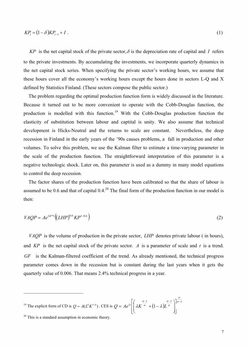
( ) IKPKP tt +−= −11 δ . (1)

KP is the net capital stock of the private sector,δ is the depreciation rate of capital and I refers

to the private investments. By accumulating the investments, we incorporate quarterly dynamics in

the net capital stock series. When specifying the private sector’s working hours, we assume that

these hours cover all the economy’s working hours except the hours done in sectors L-Q and X

defined by Statistics Finland. (These sectors compose the public sector.)

The problem regarding the optimal production function form is widely discussed in the literature.

Because it turned out to be more convenient to operate with the Cobb-Douglas function, the

production is modelled with this function.19 With the Cobb-Douglas production function the

elasticity of substitution between labour and captital is unity. We also assume that technical

development is Hicks-Neutral and the returns to scale are constant. Nevertheless, the deep

recession in Finland in the early years of the ’90s causes problems, a fall in production and other

volumes. To solve this problem, we use the Kalman filter to estimate a time-varying parameter in

the scale of the production function. The straightforward interpretation of this parameter is a

negative technologic shock. Later on, this parameter is used as a dummy in many model equations

to control the deep recession.

The factor shares of the production function have been calibrated so that the share of labour is

assumed to be 0.6 and that of capital 0.4.20 The final form of the production function in our model is

then:

( )( )6.016.0* −= KPLHPAeVAQP tGF (2)

VAQP is the volume of production in the private sector, LHP denotes private labour ( in hours),

and KP is the net capital stock of the private sector. A is a parameter of scale and t is a trend.

GF is the Kalman-filtered coefficient of the trend. As already mentioned, the technical progress

parameter comes down in the recession but is constant during the last years when it gets the

quarterly value of 0.006. That means 2.4% technical progress in a year.

19 The explicit form of CD is )( 1 bbKLAQ −= . CES is ( )111

1−−−

−+=

σσ

σσ

σσ

λ λλ LKAeQ t

20 This is a standard assumption in economic theory.

8

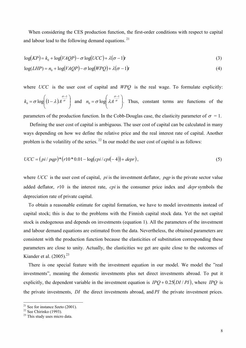
When considering the CES production function, the first-order conditions with respect to capital

and labour lead to the following demand equations. 21

( ) ( ) ( ) ( )tUCCVAQPkKP 1logloglog 0 −+−+= σλσ (3)

( ) ( ) ( )tWPQVAQPnLHP 1loglog)log( 0 −+−+= σλσ (4)

where UCC is the user cost of capital and WPQ is the real wage. To formulate explicitly:

( )

−=

−σσ

λσ1

0 1log Ak and

=

−σσ

λσ1

0 log An . Thus, constant terms are functions of the

parameters of the production function. In the Cobb-Douglas case, the elasticity parameter of σ = 1.

Defining the user cost of capital is ambiguous. The user cost of capital can be calculated in many

ways depending on how we define the relative price and the real interest rate of capital. Another

problem is the volatility of the series. 22 In our model the user cost of capital is as follows:

( ) ( )( )( )deprcpicpirpqppiUCC +−−= 4/log01.0*10*/ , (5)

where UCC is the user cost of capital, pi is the investment deflator, pqp is the private sector value

added deflator, 10r is the interest rate, cpi is the consumer price index and depr symbols the

depreciation rate of private capital.

To obtain a reasonable estimate for capital formation, we have to model investments instead of

capital stock; this is due to the problems with the Finnish capital stock data. Yet the net capital

stock is endogenous and depends on investments (equation 1). All the parameters of the investment

and labour demand equations are estimated from the data. Nevertheless, the obtained parameters are

consistent with the production function because the elasticities of substitution corresponding these

parameters are close to unity. Actually, the elasticities we get are quite close to the outcomes of

Kiander et al. (2005).23

There is one special feature with the investment equation in our model. We model the ”real

investments”, meaning the domestic investments plus net direct investments abroad. To put it

explicitly, the dependent variable in the investment equation is ( )PIDIIPQ /25.0+ , where IPQ is

the private investments, DI the direct investments abroad, and PI the private investment prices.

21 See for instance Szeto (2001). 22 See Chirinko (1993). 23 This study uses micro data.

9

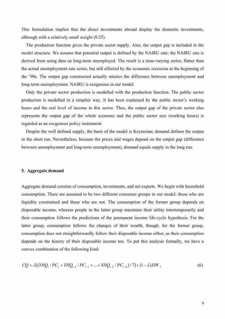
This formulation implies that the direct investments abroad display the domestic investments,

although with a relatively small weight (0.25).

The production function gives the private sector supply. Also, the output gap is included in the

model structure. We assume that potential output is defined by the NAIRU rate; the NAIRU rate is

derived from using data on long-term unemployed. The result is a time-varying series, flatter than

the actual unemployment rate series, but still affected by the economic recession at the beginning of

the ’90s. The output gap constructed actually mimics the difference between unemployment and

long-term unemployment. NAIRU is exogenous in our model.

Only the private sector production is modelled with the production function. The public sector

production is modelled in a simplier way. It has been explained by the public sector’s working

hours and the real level of income in this sector. Thus, the output gap of the private sector also

represents the output gap of the whole economy and the public sector size (working hours) is

regarded as an exogenous policy instrument.

Despite the well defined supply, the basis of the model is Keynesian; demand defines the output

in the short run. Nevertheless, because the prices and wages depend on the output gap (difference

between unemployment and long-term unemployment), demand equals supply in the long run.

5. Aggregate demand

Aggregate demand consists of consumption, investments, and net exports. We begin with household

consumption. There are assumed to be two different consumer groups in our model: those who are

liquidity constrained and those who are not. The consumption of the former group depends on

disposable income, whereas people in the latter group maximize their utility intertemporarily and

their consumption follows the predictions of the permanent income life-cycle hypothesis. For the

latter group, consumption follows the changes of their wealth, though, for the former group,

consumption does not straightforwardly follow their disposable income either, as their consumption

depends on the history of their disposable income too. To put this analysis formally, we have a

convex combination of the following kind:

( ) HWPCYHQPCYHQPCYHQCQ tttttt )1(7/)/...//( 6611 λλ −++++= −−−− , (6)

10

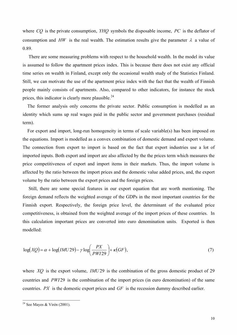
where CQ is the private consumption, YHQ symbols the disposable income, PC is the deflator of

consumption and HW is the real wealth. The estimation results give the parameter λ a value of

0.89.

There are some measuring problems with respect to the household wealth. In the model its value

is assumed to follow the apartment prices index. This is because there does not exist any official

time series on wealth in Finland, except only the occasional wealth study of the Statistics Finland.

Still, we can motivate the use of the apartment price index with the fact that the wealth of Finnish

people mainly consists of apartments. Also, compared to other indicators, for instance the stock

prices, this indicator is clearly more plausible.24

The former analysis only concerns the private sector. Public consumption is modelled as an

identity which sums up real wages paid in the public sector and government purchases (residual

term).

For export and import, long-run homogeneity in terms of scale variable(s) has been imposed on

the equations. Import is modelled as a convex combination of domestic demand and export volume.

The connection from export to import is based on the fact that export industries use a lot of

imported inputs. Both export and import are also affected by the the prices term which measures the

price competitiveness of export and import items in their markets. Thus, the import volume is

affected by the ratio between the import prices and the domestic value added prices, and, the export

volume by the ratio between the export prices and the foreign prices.

Still, there are some special features in our export equation that are worth mentioning. The

foreign demand reflects the weighted average of the GDPs in the most important countries for the

Finnish export. Respectively, the foreign price level, the determinant of the evaluated price

competitiveness, is obtained from the weighted average of the import prices of these countries. In

this calculation important prices are converted into euro denomination units. Exported is then

modelled:

( ) ( ) ( )GFPWI

PXIMUXQ κγα +

−+=

29log29loglog , (7)

where XQ is the export volume, 29IMU is the combination of the gross domestic product of 29

countries and 29PWI is the combination of the import prices (in euro denomination) of the same

countries. PX is the domestic export prices and GF is the recession dummy described earlier.

24 See Mayes & Virén (2001).

11

6. Prices and Wages

All variables which determine GDP on the demand side are expressed in real and nominal values.

For that reason, we also need to model the prices. The price block in our model is based on the law

of one price. Thus, static homogeneity has been imposed, which is equivalent to expressing the

long-run equations in terms of relative prices.

Prices are usually combinations of (private) value added prices and foreign/import prices. The

weights of individual prices have been estimated from data in all but the investment price equation.

In this equation the weights have been calibrated. It is assumed that PWI29 defined in the previous

chapter approximates to the foreign prices. Despite PWI29 also explains the export price level, our

export price equation’s fit in terms of R2 remains rather poor. For the same reason import prices are

regarded as an exogenous variable in the current version of the model.

In the price block, there is also a connection from wages to other prices. Private value added

prices are assumed to follow private sector wages (positively) and average productivity

(negatively). Then, private consumption prices react to the changes in the value added prices. This

induces a degree of sluggishness in the response of private consumption prices to changes in the

wage rate.

There are also some other (volume) variables that affect the prices in the model. For instance, the

output gap, measured as a difference between unemployment and long-term unemployment, affects

investment prices. In addition, export prices are also affected by the recession dummy and

dollar/euro exchange rate.

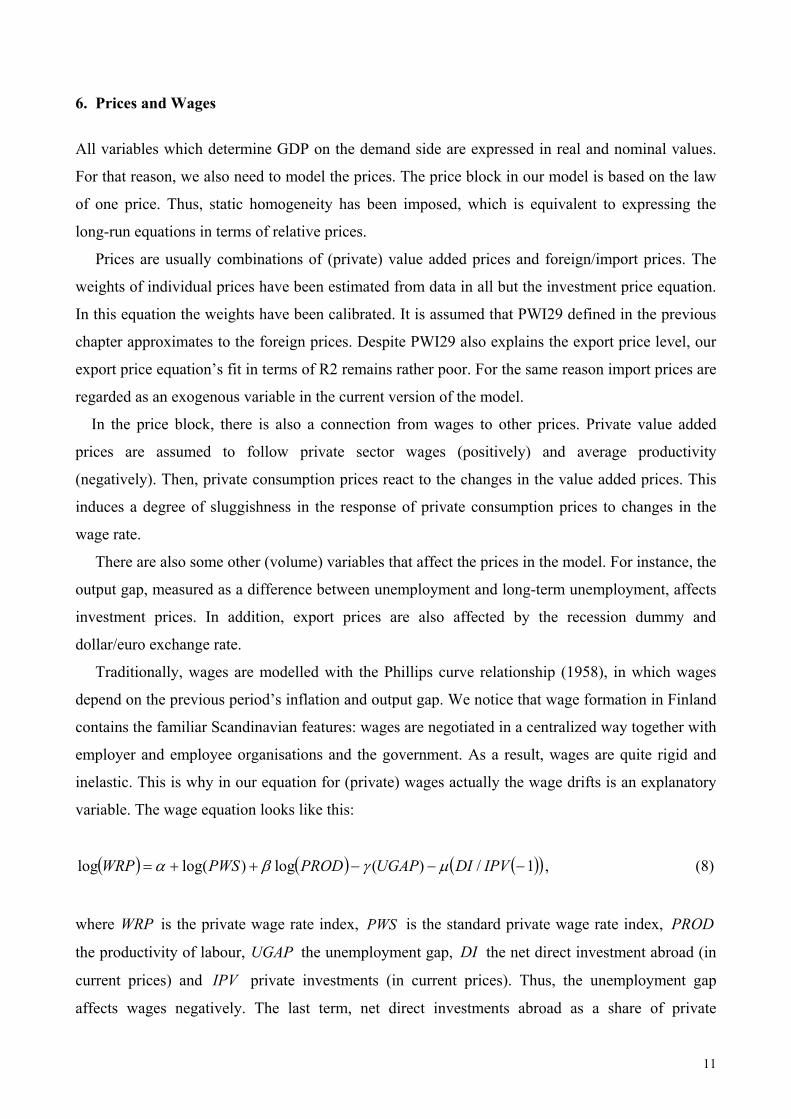
Traditionally, wages are modelled with the Phillips curve relationship (1958), in which wages

depend on the previous period’s inflation and output gap. We notice that wage formation in Finland

contains the familiar Scandinavian features: wages are negotiated in a centralized way together with

employer and employee organisations and the government. As a result, wages are quite rigid and

inelastic. This is why in our equation for (private) wages actually the wage drifts is an explanatory

variable. The wage equation looks like this:

( ) ( ) ( )( )1/)(log)log(log −−−++= IPVDIUGAPPRODPWSWRP µγβα , (8)

where WRP is the private wage rate index, PWS is the standard private wage rate index, PROD

the productivity of labour, UGAP the unemployment gap, DI the net direct investment abroad (in

current prices) and IPV private investments (in current prices). Thus, the unemployment gap

affects wages negatively. The last term, net direct investments abroad as a share of private

12

investments, demands further explanation. Despite the rigidities in Finnish wage formation it has

been assumed that direct investments abroad create a negative pressure on domestic wages.

According to the data the impact is rather small, but statistically significant.

To capture the labour market effects properly, we also endogenise the standard private wage rate

index. It is explained by the combination of its lagged value and the private consumption prices, and

the output gap (its one-year moving average). In our model the public sector wages follow the

private sector wages and the output gap has a negative effect on the public sector wages.

7. Income accounting and public sector

The public sector, its revenues and expenditures, is mainly modelled with identities. The same

applies to the income accounting of households. Since the model has been planned to be used as a

forecasting tool at the Labour Institute for Economic Research, the identities are constructed with

the help of the Institute’s forecasting system. To avoid of making the model system too

complicated, some identities have been constructed outside the model. For instance, employers

contributions to the social security was originally calculated in Excel by adding up the employer’s

actual and imputed social contributions.

When the public sector and income accounting identities were being constructed, the main aim

was to make them consistent with the national accounts data. The identities also describe the legal

and institutional framework of the public sector. Public sector linkages are important in all policy

simulations.

In the public sector, behavioural equations are estimated only for value added, wages, and

consumption prices. Still, this is not the whole truth, since the parameters in the public sector

identities are usually estimated from the data. The residual terms received from the estimations are

added in the public sector identities. The typical form of a public sector identity then is

( ) RESIDCVTAXQM ++= log)log( βα , (9)

where TAXQM denotes the production and import taxes collected by the public sector. They

depend on private consumption in current terms (CV ); the parameter β has been estimated from

the data. RESID is the residual term which makes the right side of the equation consistent with the

left side.

13

8. Some policy simulations with EMMA

The following illustrative policy simulations are reported in this paper

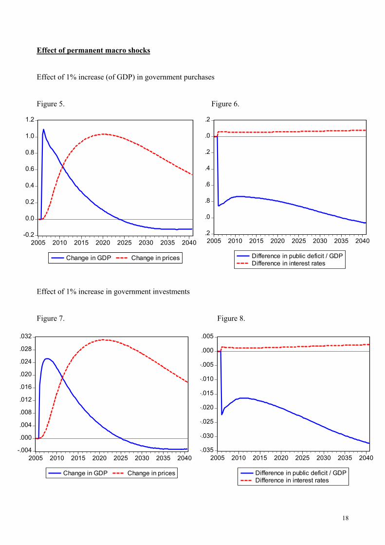
- an increase of government purchases by 1 per cent (of GDP)

- an increase of government investments by 1 per cent

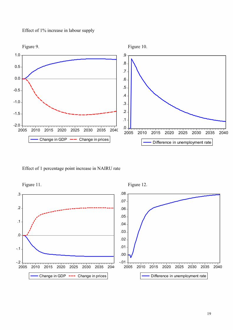
- an increase of labour supply by 1 per cent

- an increase of NAIRU rate by 1 percentage point

- an increase of interest rates by 1 percentage point

- an increase of foreign demand by 1 per cent

- an increase of VAT rate by 1 percentage point

- a revaluation of euro/dollar exchange rate by 10 per cent

All simulations are carried out in the case of fixed exchange rate and without any policy rules. The

simulations show that the model has reasonable short-term and medium-term properties. Although

the short-run effects are definitely Keynesian (see eg the fiscal multipliers), the long-run effects are

dominantly supply oriented. Thus, in the long run, expansive fiscal policies - increases in

government purchases and government investments - lead to contradictory output effects. This is

mainly due to the deterioration of the real exhange rate. We also notice that the increase in the

public deficit affects the yield on government bonds; this way it affects the other parts of the

economy, private investments for instance. In addition, the fiscal shocks lead to major public sector

imbalances in the long run. Nevertheless, one has to remember that in the current version of the

model there is no link between public sector investments and private sector productivity. If it is

assumed that the public investments increase the private productivity, the (public investment)

shock’s impact on output may not be contradictory in the long run.

Also, some labour market shocks are scrutinized. At first, a 1% increase in labour supply goes to

the unemployment; at the same time, the output gap of the economy becomes smaller ( economy is

further from its potential). As a consequence, the negotiation power of the employee organizations

decreases and the wages start to fall. This improves the demand for labour and boosts the total

supply in the economy. In the long run, also other prices in the economy fall due to the decrease in

the nominal wages. The decrease in the domestic price level advances the export sector

competitiveness and increases the real wages. In the long run, a shock on labour supply is matched

by nearly proportional increase in the output volume. This is a standard outcome in the small open

economy model.

14

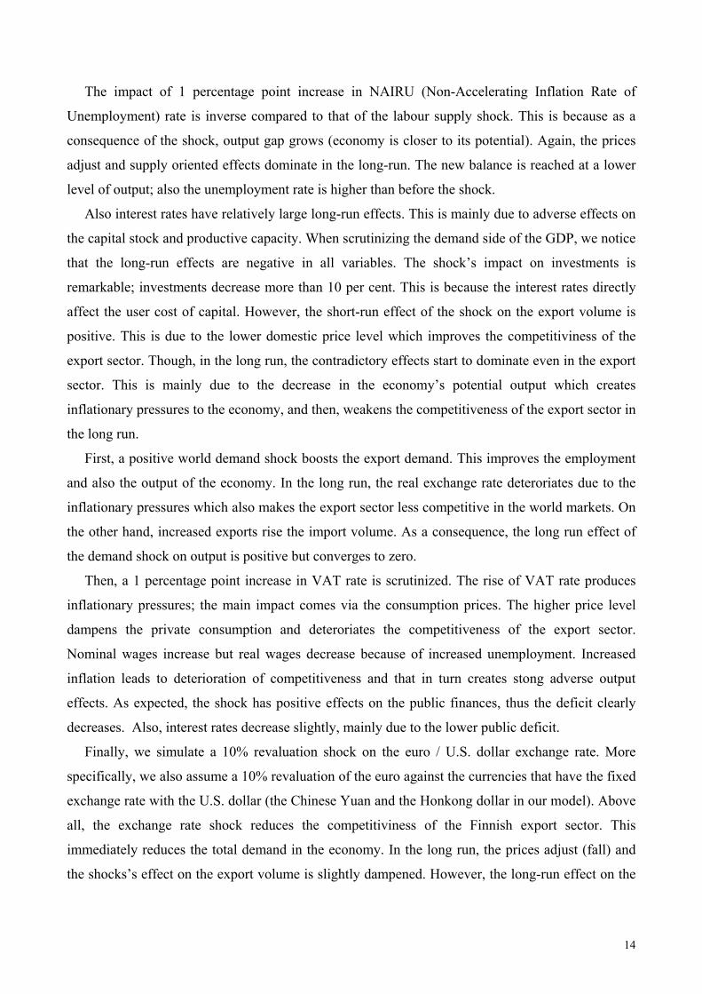
The impact of 1 percentage point increase in NAIRU (Non-Accelerating Inflation Rate of

Unemployment) rate is inverse compared to that of the labour supply shock. This is because as a

consequence of the shock, output gap grows (economy is closer to its potential). Again, the prices

adjust and supply oriented effects dominate in the long-run. The new balance is reached at a lower

level of output; also the unemployment rate is higher than before the shock.

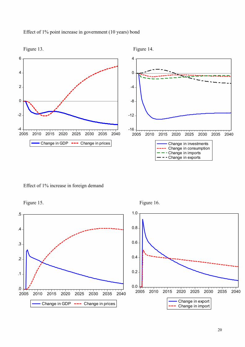
Also interest rates have relatively large long-run effects. This is mainly due to adverse effects on

the capital stock and productive capacity. When scrutinizing the demand side of the GDP, we notice

that the long-run effects are negative in all variables. The shock’s impact on investments is

remarkable; investments decrease more than 10 per cent. This is because the interest rates directly

affect the user cost of capital. However, the short-run effect of the shock on the export volume is

positive. This is due to the lower domestic price level which improves the competitiviness of the

export sector. Though, in the long run, the contradictory effects start to dominate even in the export

sector. This is mainly due to the decrease in the economy’s potential output which creates

inflationary pressures to the economy, and then, weakens the competitiveness of the export sector in

the long run.

First, a positive world demand shock boosts the export demand. This improves the employment

and also the output of the economy. In the long run, the real exchange rate deteroriates due to the

inflationary pressures which also makes the export sector less competitive in the world markets. On

the other hand, increased exports rise the import volume. As a consequence, the long run effect of

the demand shock on output is positive but converges to zero.

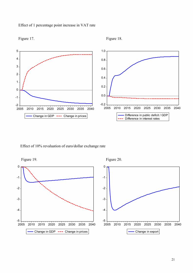
Then, a 1 percentage point increase in VAT rate is scrutinized. The rise of VAT rate produces

inflationary pressures; the main impact comes via the consumption prices. The higher price level

dampens the private consumption and deteroriates the competitiveness of the export sector.

Nominal wages increase but real wages decrease because of increased unemployment. Increased

inflation leads to deterioration of competitiveness and that in turn creates stong adverse output

effects. As expected, the shock has positive effects on the public finances, thus the deficit clearly

decreases. Also, interest rates decrease slightly, mainly due to the lower public deficit.

Finally, we simulate a 10% revaluation shock on the euro / U.S. dollar exchange rate. More

specifically, we also assume a 10% revaluation of the euro against the currencies that have the fixed

exchange rate with the U.S. dollar (the Chinese Yuan and the Honkong dollar in our model). Above

all, the exchange rate shock reduces the competitiviness of the Finnish export sector. This

immediately reduces the total demand in the economy. In the long run, the prices adjust (fall) and

the shocks’s effect on the export volume is slightly dampened. However, the long-run effect on the

15

output is negative because the shock reduces both the capital stock and the demand for labour.

Thus, after 35 years, GDP is more than 1% lower than before the shock.

9. Concluding remarks

Forecasting models are never ready. This is also true with the Labour Institute's model. Even so, the

current model can already be used in actual forecasting work. This practical work also gives

valueable information for the future development of the model. It is hoped that a more complete

model version can be constructed during the year 2007. After doing that, also a more complete

report on the structure and properties of the model can be published.

16

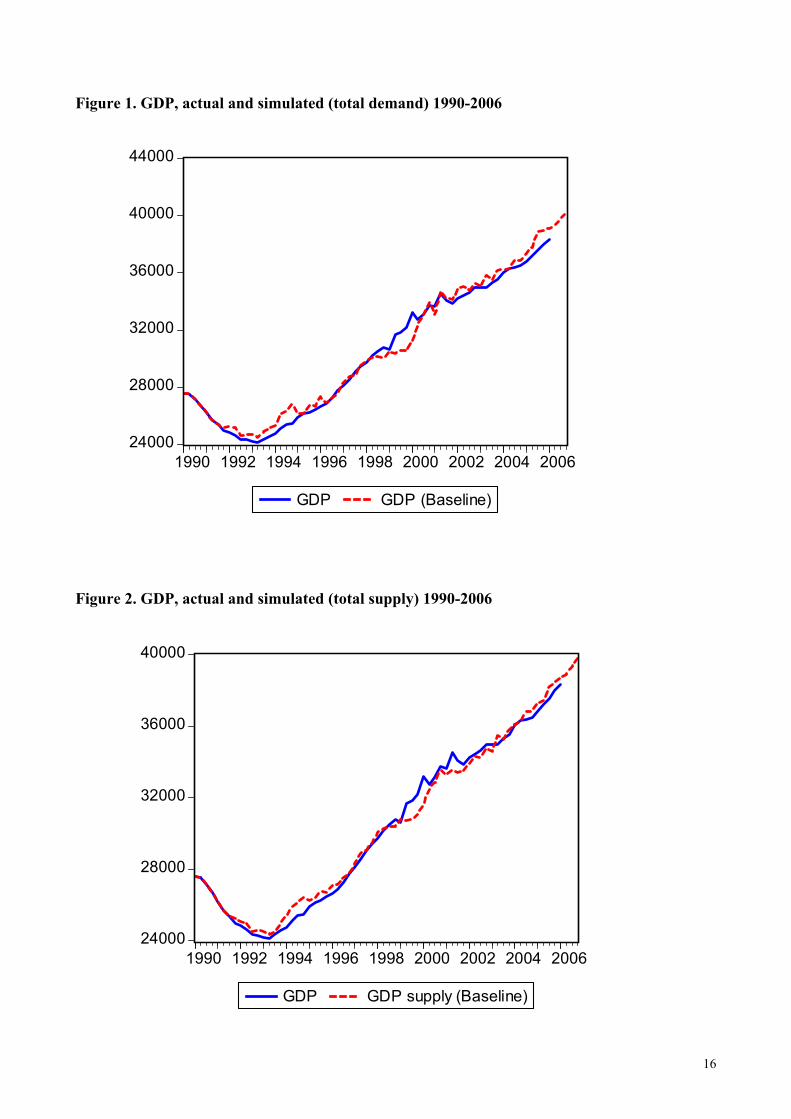
Figure 1. GDP, actual and simulated (total demand) 1990-2006

Figure 2. GDP, actual and simulated (total supply) 1990-2006

24000

28000

32000

36000

40000

44000

1990 1992 1994 1996 1998 2000 2002 2004 2006

GDP GDP (Baseline)

24000

28000

32000

36000

40000

1990 1992 1994 1996 1998 2000 2002 2004 2006

GDP GDP supply (Baseline)

17

20000

40000

60000

80000

100000

120000

140000

160000

180000

90 95 00 05 10 15 20 25 30 35 40

GDP (Baseline)GDP (Baseline Mean)GDP (Baseline Mean) + 2 * sdGDP (Baseline Mean) - 2 * sd

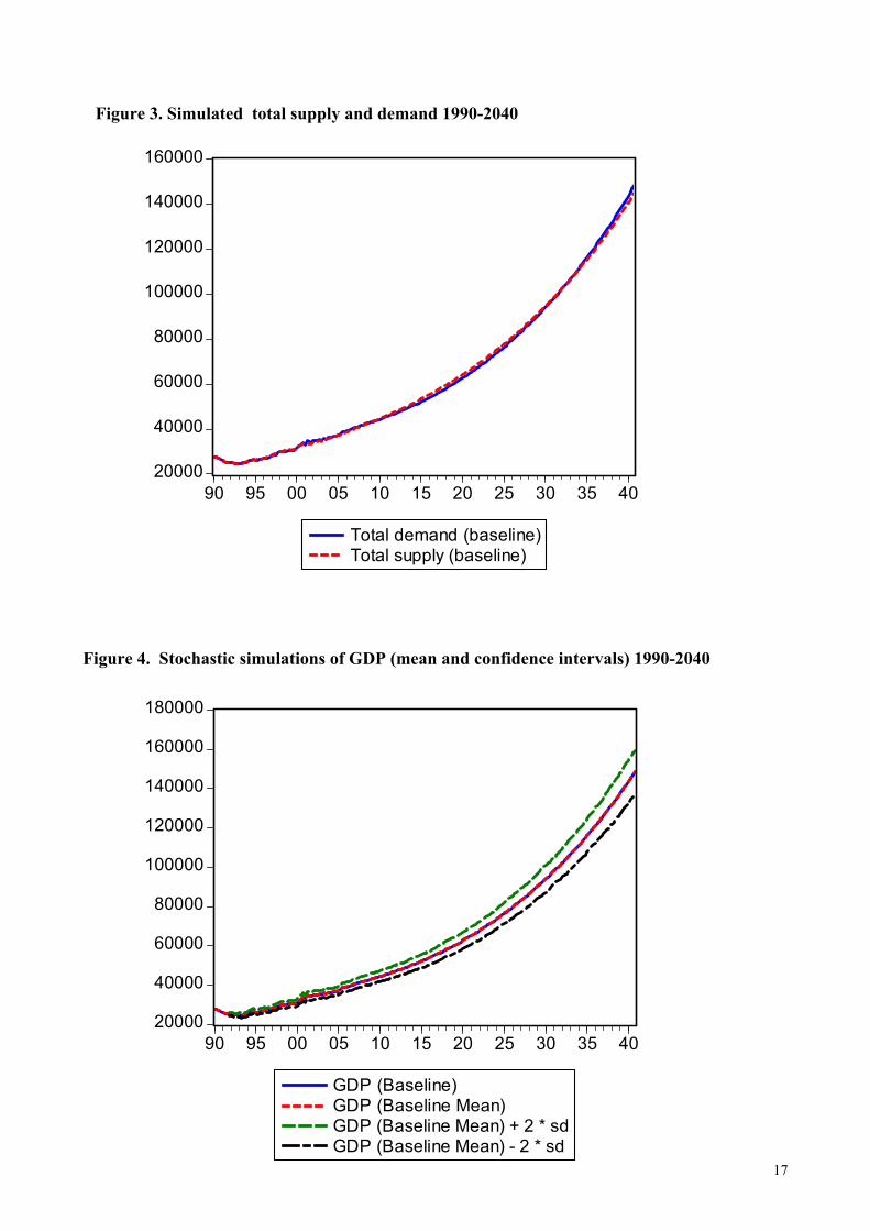
Figure 3. Simulated total supply and demand 1990-2040

Figure 4. Stochastic simulations of GDP (mean and confidence intervals) 1990-2040

20000

40000

60000

80000

100000

120000

140000

160000

90 95 00 05 10 15 20 25 30 35 40

Total demand (baseline)Total supply (baseline)

18

Effect of permanent macro shocks

Effect of 1% increase (of GDP) in government purchases

Figure 5. Figure 6.

Effect of 1% increase in government investments

Figure 7. Figure 8.

-1.2

-1.0

-0.8

-0.6

-0.4

-0.2

0.0

0.2

2005 2010 2015 2020 2025 2030 2035 2040

Difference in public deficit / GDPDifference in interest rates

-.035

-.030

-.025

-.020

-.015

-.010

-.005

.000

.005

2005 2010 2015 2020 2025 2030 2035 2040

Difference in public deficit / GDPDifference in interest rates

-0.2

0.0

0.2

0.4

0.6

0.8

1.0

1.2

2005 2010 2015 2020 2025 2030 2035 2040

Change in GDP Change in prices

-.004

.000

.004

.008

.012

.016

.020

.024

.028

.032

2005 2010 2015 2020 2025 2030 2035 2040

Change in GDP Change in prices

19

Effect of 1% increase in labour supply

Figure 9. Figure 10.

Effect of 1 percentage point increase in NAIRU rate

Figure 11. Figure 12.

Effect of 1% point increase in government (10 years) bond

-2.0

-1.5

-1.0

-0.5

0.0

0.5

1.0

2005 2010 2015 2020 2025 2030 2035 2040

Change in GDP Change in prices

.0

.1

.2

.3

.4

.5

.6

.7

.8

.9

2005 2010 2015 2020 2025 2030 2035 2040

Difference in unemployment rate

-.2

-.1

.0

.1

.2

.3

2005 2010 2015 2020 2025 2030 2035 2040

Change in GDP Change in prices

-.01

.00

.01

.02

.03

.04

.05

.06

.07

.08

2005 2010 2015 2020 2025 2030 2035 2040

Difference in unemployment rate

20

Effect of 1% point increase in government (10 years) bond

Figure 13. Figure 14.

Effect of 1% increase in foreign demand

Figure 15. Figure 16.

.0

.1

.2

.3

.4

.5

2005 2010 2015 2020 2025 2030 2035 2040

Change in GDP Change in prices

0.0

0.2

0.4

0.6

0.8

1.0

2005 2010 2015 2020 2025 2030 2035 2040

Change in exportChange in import

-16

-12

-8

-4

0

4

2005 2010 2015 2020 2025 2030 2035 2040

Change in investmentsChange in consumption Change in importsChange in exports

-4

-2

0

2

4

6

2005 2010 2015 2020 2025 2030 2035 2040

Change in GDP Change in prices

21

Effect of 1 percentage point increase in VAT rate

Figure 17. Figure 18.

Effect of 10% revaluation of euro/dollar exchange rate

Figure 19. Figure 20.

-2

-1

0

1

2

3

4

5

2005 2010 2015 2020 2025 2030 2035 2040

Change in GDP Change in prices

-0.2

0.0

0.2

0.4

0.6

0.8

1.0

2005 2010 2015 2020 2025 2030 2035 2040

Difference in public deficit / GDPDifference in interest rates

-5

-4

-3

-2

-1

0

2005 2010 2015 2020 2025 2030 2035 2040

Change in GDP Change in prices

-5

-4

-3

-2

-1

0

2005 2010 2015 2020 2025 2030 2035 2040

Change in export

22

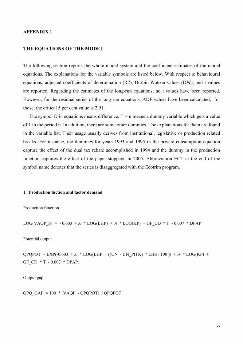
APPENDIX 1

THE EQUATIONS OF THE MODEL

The following section reports the whole model system and the coefficient estimates of the model

equations. The explanations for the variable symbols are listed below. With respect to behavioural

equations, adjusted coefficients of determination (R2), Durbin-Watson values (DW), and t-values

are reported. Regarding the estimates of the long-run equations, no t values have been reported.

However, for the residual series of the long-run equations, ADF values have been calculated; for

those, the critical 5 per cent value is 2.91.

The symbol D in equations means difference. T = n means a dummy variable which gets a value

of 1 in the period n. In addition, there are some other dummies. The explanations for them are found

in the variable list. Their usage usually derives from institutional, legislative or production related

breaks. For instance, the dummies for years 1993 and 1995 in the private consumption equation

capture the effect of the dual tax rebate accomplished in 1994 and the dummy in the production

function captures the effect of the paper stoppage in 2005. Abbreviation ECT at the end of the

symbol name denotes that the series is disaggregated with the Ecotrim program.

1. Production fuction and factor demand

Production function

LOG(VAQP_S) = - 0.603 + .6 * LOG(LHP) + .4 * LOG(KP) + GF_CD * T - 0.007 * DPAP

Potential output

QPQPOT = EXP(-0.603 + .6 * LOG(LHP + ((UN - UN_PITK) * LHS / 100 )) + .4 * LOG(KP) +

GF_CD * T - 0.007 * DPAP)

Output gap

QPQ_GAP = 100 * (VAQP - QPQPOT) / QPQPOT

23

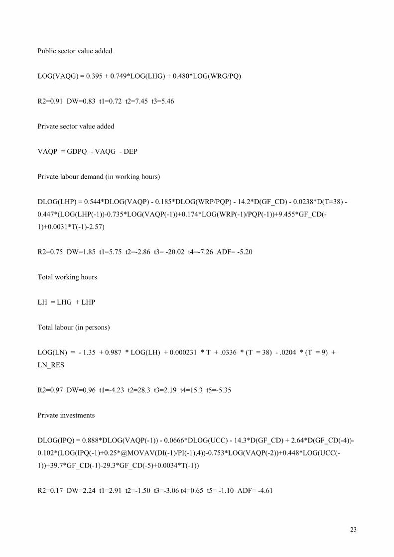
Public sector value added

LOG(VAQG) = 0.395 + 0.749*LOG(LHG) + 0.480*LOG(WRG/PQ)

R2=0.91 DW=0.83 t1=0.72 t2=7.45 t3=5.46

Private sector value added

VAQP = GDPQ - VAQG - DEP

Private labour demand (in working hours)

DLOG(LHP) = 0.544*DLOG(VAQP) - 0.185*DLOG(WRP/PQP) - 14.2*D(GF_CD) - 0.0238*D(T=38) -

0.447*(LOG(LHP(-1))-0.735*LOG(VAQP(-1))+0.174*LOG(WRP(-1)/PQP(-1))+9.455*GF_CD(-

1)+0.0031*T(-1)-2.57)

R2=0.75 DW=1.85 t1=5.75 t2=-2.86 t3= -20.02 t4=-7.26 ADF= -5.20

Total working hours

LH = LHG + LHP

Total labour (in persons)

LOG(LN) = - 1.35 + 0.987 * LOG(LH) + 0.000231 * T + .0336 * (T = 38) - .0204 * (T = 9) +

LN_RES

R2=0.97 DW=0.96 t1=-4.23 t2=28.3 t3=2.19 t4=15.3 t5=-5.35

Private investments

DLOG(IPQ) = 0.888*DLOG(VAQP(-1)) - 0.0666*DLOG(UCC) - 14.3*D(GF_CD) + 2.64*D(GF_CD(-4))-

0.102*(LOG(IPQ(-1)+0.25*@MOVAV(DI(-1)/PI(-1),4))-0.753*LOG(VAQP(-2))+0.448*LOG(UCC(-

1))+39.7*GF_CD(-1)-29.3*GF_CD(-5)+0.0034*T(-1))

R2=0.17 DW=2.24 t1=2.91 t2=-1.50 t3=-3.06 t4=0.65 t5= -1.10 ADF= -4.61

24

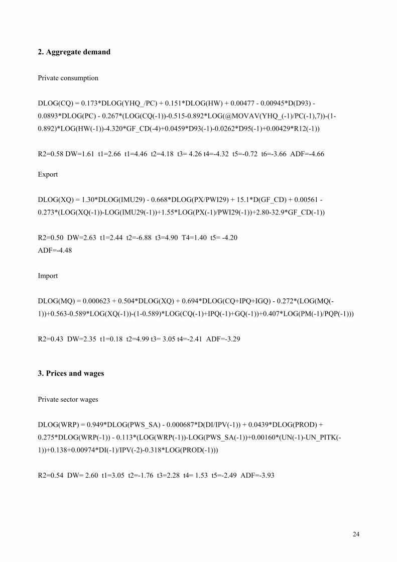
2. Aggregate demand

Private consumption

DLOG(CQ) = 0.173*DLOG(YHQ_/PC) + 0.151*DLOG(HW) + 0.00477 - 0.00945*D(D93) -

0.0893*DLOG(PC) - 0.267*(LOG(CQ(-1))-0.515-0.892*LOG(@MOVAV(YHQ_(-1)/PC(-1),7))-(1-

0.892)*LOG(HW(-1))-4.320*GF_CD(-4)+0.0459*D93(-1)-0.0262*D95(-1)+0.00429*R12(-1))

R2=0.58 DW=1.61 t1=2.66 t1=4.46 t2=4.18 t3= 4.26 t4=-4.32 t5=-0.72 t6=-3.66 ADF=-4.66

Export

DLOG(XQ) = 1.30*DLOG(IMU29) - 0.668*DLOG(PX/PWI29) + 15.1*D(GF_CD) + 0.00561 -

0.273*(LOG(XQ(-1))-LOG(IMU29(-1))+1.55*LOG(PX(-1)/PWI29(-1))+2.80-32.9*GF_CD(-1))

R2=0.50 DW=2.63 t1=2.44 t2=-6.88 t3=4.90 T4=1.40 t5= -4.20

ADF=-4.48

Import

DLOG(MQ) = 0.000623 + 0.504*DLOG(XQ) + 0.694*DLOG(CQ+IPQ+IGQ) - 0.272*(LOG(MQ(-

1))+0.563-0.589*LOG(XQ(-1))-(1-0.589)*LOG(CQ(-1)+IPQ(-1)+GQ(-1))+0.407*LOG(PM(-1)/PQP(-1)))

R2=0.43 DW=2.35 t1=0.18 t2=4.99 t3= 3.05 t4=-2.41 ADF=-3.29

3. Prices and wages

Private sector wages

DLOG(WRP) = 0.949*DLOG(PWS_SA) - 0.000687*D(DI/IPV(-1)) + 0.0439*DLOG(PROD) +

0.275*DLOG(WRP(-1)) - 0.113*(LOG(WRP(-1))-LOG(PWS_SA(-1))+0.00160*(UN(-1)-UN_PITK(-

1))+0.138+0.00974*DI(-1)/IPV(-2)-0.318*LOG(PROD(-1)))

R2=0.54 DW= 2.60 t1=3.05 t2=-1.76 t3=2.28 t4= 1.53 t5=-2.49 ADF=-3.93

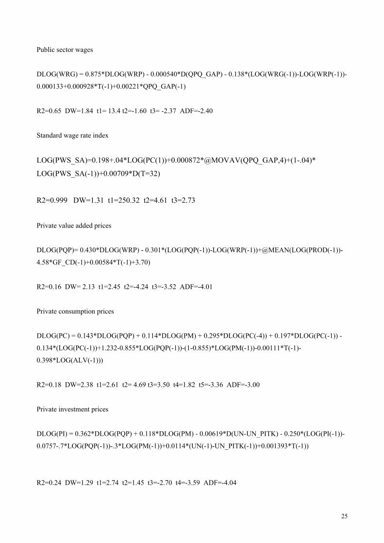
25

Public sector wages

DLOG(WRG) = 0.875*DLOG(WRP) - 0.000540*D(QPQ_GAP) - 0.138*(LOG(WRG(-1))-LOG(WRP(-1))-

0.000133+0.000928*T(-1)+0.00221*QPQ_GAP(-1)

R2=0.65 DW=1.84 t1= 13.4 t2=-1.60 t3= -2.37 ADF=-2.40

Standard wage rate index

LOG(PWS_SA)=0.198+.04*LOG(PC(1))+0.000872*@MOVAV(QPQ_GAP,4)+(1-.04)*

LOG(PWS_SA(-1))+0.00709*D(T=32)

R2=0.999 DW=1.31 t1=250.32 t2=4.61 t3=2.73

Private value added prices

DLOG(PQP)= 0.430*DLOG(WRP) - 0.301*(LOG(PQP(-1))-LOG(WRP(-1))+@MEAN(LOG(PROD(-1))-

4.58*GF_CD(-1)+0.00584*T(-1)+3.70)

R2=0.16 DW= 2.13 t1=2.45 t2=-4.24 t3=-3.52 ADF=-4.01

Private consumption prices

DLOG(PC) = 0.143*DLOG(PQP) + 0.114*DLOG(PM) + 0.295*DLOG(PC(-4)) + 0.197*DLOG(PC(-1)) -

0.134*(LOG(PC(-1))+1.232-0.855*LOG(PQP(-1))-(1-0.855)*LOG(PM(-1))-0.00111*T(-1)-

0.398*LOG(ALV(-1)))

R2=0.18 DW=2.38 t1=2.61 t2= 4.69 t3=3.50 t4=1.82 t5=-3.36 ADF=-3.00

Private investment prices

DLOG(PI) = 0.362*DLOG(PQP) + 0.118*DLOG(PM) - 0.00619*D(UN-UN_PITK) - 0.250*(LOG(PI(-1))-

0.0757-.7*LOG(PQP(-1))-.3*LOG(PM(-1))+0.0114*(UN(-1)-UN_PITK(-1))+0.001393*T(-1))

R2=0.24 DW=1.29 t1=2.74 t2=1.45 t3=-2.70 t4=-3.59 ADF=-4.04

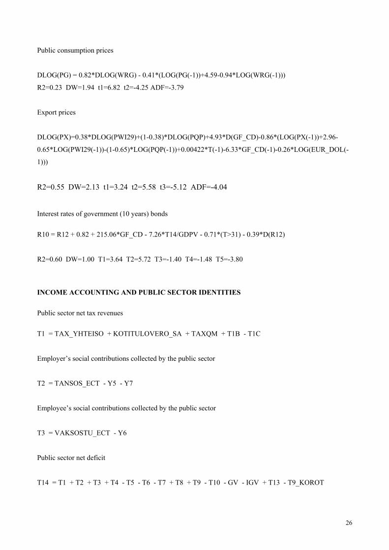
26

Public consumption prices

DLOG(PG) = 0.82*DLOG(WRG) - 0.41*(LOG(PG(-1))+4.59-0.94*LOG(WRG(-1)))

R2=0.23 DW=1.94 t1=6.82 t2=-4.25 ADF=-3.79

Export prices

DLOG(PX)=0.38*DLOG(PWI29)+(1-0.38)*DLOG(PQP)+4.93*D(GF_CD)-0.86*(LOG(PX(-1))+2.96-

0.65*LOG(PWI29(-1))-(1-0.65)*LOG(PQP(-1))+0.00422*T(-1)-6.33*GF_CD(-1)-0.26*LOG(EUR_DOL(-

1)))

R2=0.55 DW=2.13 t1=3.24 t2=5.58 t3=-5.12 ADF=-4.04

Interest rates of government (10 years) bonds

R10 = R12 + 0.82 + 215.06*GF_CD - 7.26*T14/GDPV - 0.71*(T>31) - 0.39*D(R12)

R2=0.60 DW=1.00 T1=3.64 T2=5.72 T3=-1.40 T4=-1.48 T5=-3.80

INCOME ACCOUNTING AND PUBLIC SECTOR IDENTITIES

Public sector net tax revenues

T1 = TAX_YHTEISO + KOTITULOVERO_SA + TAXQM + T1B - T1C

Employer’s social contributions collected by the public sector

T2 = TANSOS_ECT - Y5 - Y7

Employee’s social contributions collected by the public sector

T3 = VAKSOSTU_ECT - Y6

Public sector net deficit

T14 = T1 + T2 + T3 + T4 - T5 - T6 - T7 + T8 + T9 - T10 - GV - IGV + T13 - T9_KOROT

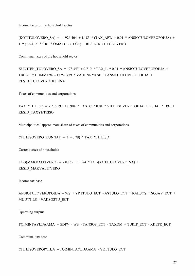
27

Income taxes of the household sector

(KOTITULOVERO_SA) = - 1926.404 + 1.183 * (TAX_APW * 0.01 * ANSIOTULOVEROPOHJA) +

1 * (TAX_K * 0.01 * OMATULO_ECT) + RESID_KOTITULOVERO

Communal taxes of the household sector

KUNTIEN_TULOVERO_SA = 173.347 + 0.719 * TAX_L * 0.01 * ANSIOTULOVEROPOHJA +

118.320 * DUMMY94 - 17757.779 * VAHENNYKSET / ANSIOTULOVEROPOHJA +

RESID_TULOVERO_KUNNAT

Taxes of communities and corporations

TAX_YHTEISO = - 236.197 + 0.904 * TAX_C * 0.01 * YHTEISOVEROPOHJA + 117.141 * D92 +

RESID_TAXYHTEISO

Municipalities’ approximate share of taxes of communities and corporations

YHTEISOVERO_KUNNAT = (1 - 0.79) * TAX_YHTEISO

Current taxes of households

LOG(MAKVALITVERO) = - 0.159 + 1.024 * LOG(KOTITULOVERO_SA) +

RESID_MAKVALITVERO

Income tax base

ANSIOTULOVEROPOHJA = WS + YRTTULO_ECT - ASTULO_ECT + RAHSOS + SOSAV_ECT +

MUUTTILS - VAKSOSTU_ECT

Operating surplus

TOIMINTAYLIJAAMA = GDPV - WS - TANSOS_ECT - TAXQM + TUKIP_ECT - KDEPR_ECT

Communal tax base

YHTEISOVEROPOHJA = TOIMINTAYLIJAAMA - YRTTULO_ECT

28

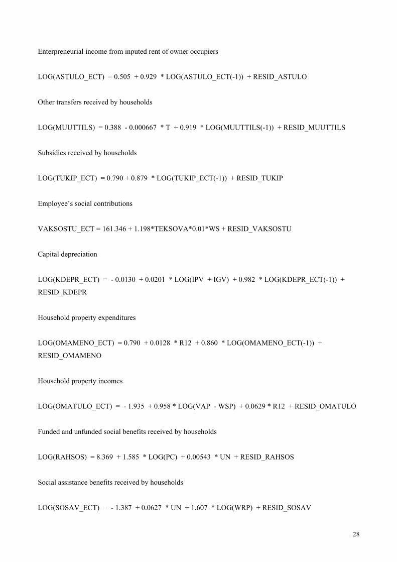
Enterpreneurial income from inputed rent of owner occupiers

LOG(ASTULO_ECT) = 0.505 + 0.929 * LOG(ASTULO_ECT(-1)) + RESID_ASTULO

Other transfers received by households

LOG(MUUTTILS) = 0.388 - 0.000667 * T + 0.919 * LOG(MUUTTILS(-1)) + RESID_MUUTTILS

Subsidies received by households

LOG(TUKIP_ECT) = 0.790 + 0.879 * LOG(TUKIP_ECT(-1)) + RESID_TUKIP

Employee’s social contributions

VAKSOSTU_ECT = 161.346 + 1.198*TEKSOVA*0.01*WS + RESID_VAKSOSTU

Capital depreciation

LOG(KDEPR_ECT) = - 0.0130 + 0.0201 * LOG(IPV + IGV) + 0.982 * LOG(KDEPR_ECT(-1)) +

RESID_KDEPR

Household property expenditures

LOG(OMAMENO_ECT) = 0.790 + 0.0128 * R12 + 0.860 * LOG(OMAMENO_ECT(-1)) +

RESID_OMAMENO

Household property incomes

LOG(OMATULO_ECT) = - 1.935 + 0.958 * LOG(VAP - WSP) + 0.0629 * R12 + RESID_OMATULO

Funded and unfunded social benefits received by households

LOG(RAHSOS) = 8.369 + 1.585 * LOG(PC) + 0.00543 * UN + RESID_RAHSOS

Social assistance benefits received by households

LOG(SOSAV_ECT) = - 1.387 + 0.0627 * UN + 1.607 * LOG(WRP) + RESID_SOSAV

29

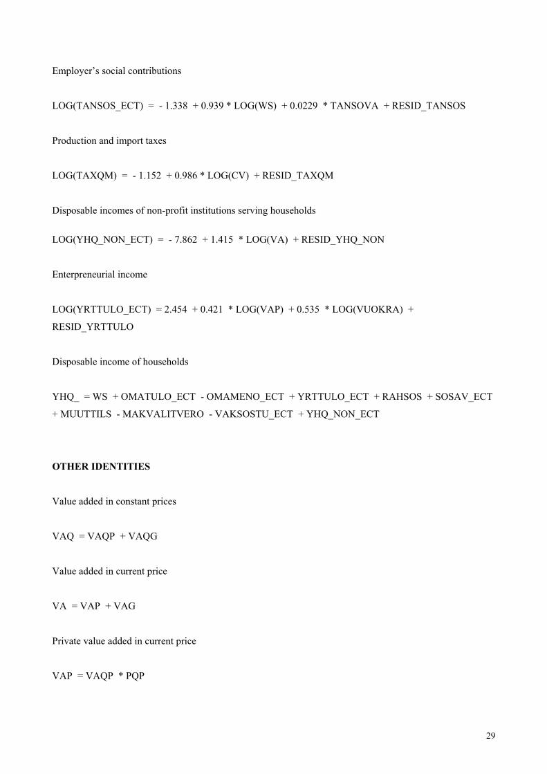
Employer’s social contributions

LOG(TANSOS_ECT) = - 1.338 + 0.939 * LOG(WS) + 0.0229 * TANSOVA + RESID_TANSOS

Production and import taxes

LOG(TAXQM) = - 1.152 + 0.986 * LOG(CV) + RESID_TAXQM

Disposable incomes of non-profit institutions serving households

LOG(YHQ_NON_ECT) = - 7.862 + 1.415 * LOG(VA) + RESID_YHQ_NON

Enterpreneurial income

LOG(YRTTULO_ECT) = 2.454 + 0.421 * LOG(VAP) + 0.535 * LOG(VUOKRA) +

RESID_YRTTULO

Disposable income of households

YHQ_ = WS + OMATULO_ECT - OMAMENO_ECT + YRTTULO_ECT + RAHSOS + SOSAV_ECT

+ MUUTTILS - MAKVALITVERO - VAKSOSTU_ECT + YHQ_NON_ECT

OTHER IDENTITIES

Value added in constant prices

VAQ = VAQP + VAQG

Value added in current price

VA = VAP + VAG

Private value added in current price

VAP = VAQP * PQP

30

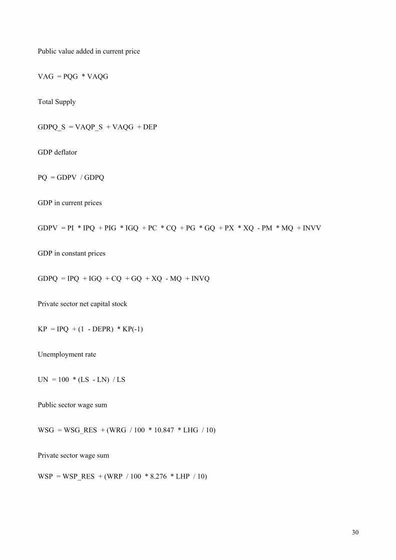
Public value added in current price

VAG = PQG * VAQG

Total Supply

GDPQ_S = VAQP_S + VAQG + DEP

GDP deflator

PQ = GDPV / GDPQ

GDP in current prices

GDPV = PI * IPQ + PIG * IGQ + PC * CQ + PG * GQ + PX * XQ - PM * MQ + INVV

GDP in constant prices

GDPQ = IPQ + IGQ + CQ + GQ + XQ - MQ + INVQ

Private sector net capital stock

KP = IPQ + (1 - DEPR) * KP(-1)

Unemployment rate

UN = 100 * (LS - LN) / LS

Public sector wage sum

WSG = WSG_RES + (WRG / 100 * 10.847 * LHG / 10)

Private sector wage sum

WSP = WSP_RES + (WRP / 100 * 8.276 * LHP / 10)

31

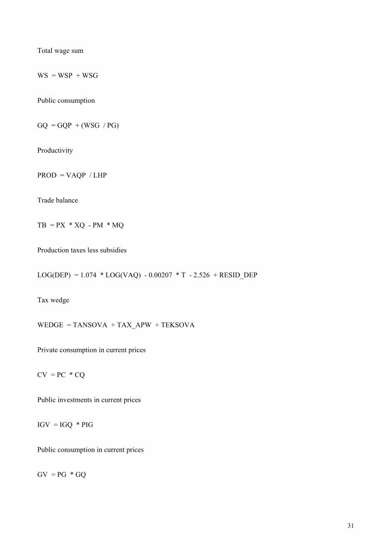
Total wage sum

WS = WSP + WSG

Public consumption

GQ = GQP + (WSG / PG)

Productivity

PROD = VAQP / LHP

Trade balance

TB = PX * XQ - PM * MQ

Production taxes less subsidies

LOG(DEP) = 1.074 * LOG(VAQ) - 0.00207 * T - 2.526 + RESID_DEP

Tax wedge

WEDGE = TANSOVA + TAX_APW + TEKSOVA

Private consumption in current prices

CV = PC * CQ

Public investments in current prices

IGV = IGQ * PIG

Public consumption in current prices

GV = PG * GQ

32

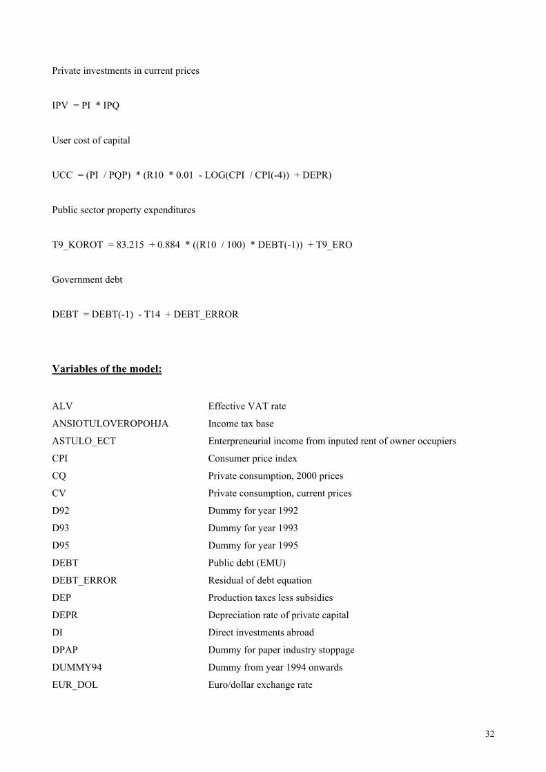
Private investments in current prices

IPV = PI * IPQ

User cost of capital

UCC = (PI / PQP) * (R10 * 0.01 - LOG(CPI / CPI(-4)) + DEPR)

Public sector property expenditures

T9_KOROT = 83.215 + 0.884 * ((R10 / 100) * DEBT(-1)) + T9_ERO

Government debt

DEBT = DEBT(-1) - T14 + DEBT_ERROR

Variables of the model:

ALV Effective VAT rate

ANSIOTULOVEROPOHJA Income tax base

ASTULO_ECT Enterpreneurial income from inputed rent of owner occupiers

CPI Consumer price index

CQ Private consumption, 2000 prices

CV Private consumption, current prices

D92 Dummy for year 1992

D93 Dummy for year 1993

D95 Dummy for year 1995

DEBT Public debt (EMU)

DEBT_ERROR Residual of debt equation

DEP Production taxes less subsidies

DEPR Depreciation rate of private capital

DI Direct investments abroad

DPAP Dummy for paper industry stoppage

DUMMY94 Dummy from year 1994 onwards

EUR_DOL Euro/dollar exchange rate

33

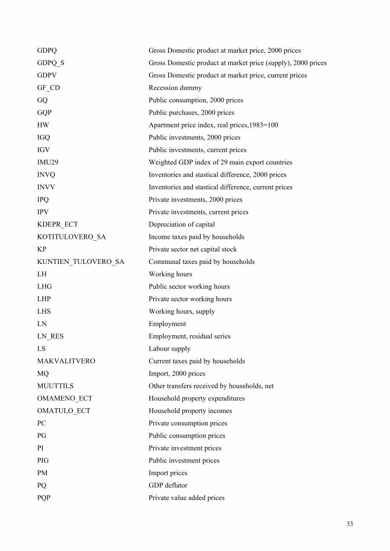
GDPQ Gross Domestic product at market price, 2000 prices

GDPQ_S Gross Domestic product at market price (supply), 2000 prices

GDPV Gross Domestic product at market price, current prices

GF_CD Recession dummy

GQ Public consumption, 2000 prices

GQP Public purchases, 2000 prices

HW Apartment price index, real prices,1983=100

IGQ Public investments, 2000 prices

IGV Public investments, current prices

IMU29 Weighted GDP index of 29 main export countries

INVQ Inventories and stastical difference, 2000 prices

INVV Inventories and stastical difference, current prices

IPQ Private investments, 2000 prices

IPV Private investments, current prices

KDEPR_ECT Depreciation of capital

KOTITULOVERO_SA Income taxes paid by households

KP Private sector net capital stock

KUNTIEN_TULOVERO_SA Communal taxes paid by households

LH Working hours

LHG Public sector working hours

LHP Private sector working hours

LHS Working hours, supply

LN Employment

LN_RES Employment, residual series

LS Labour supply

MAKVALITVERO Current taxes paid by households

MQ Import, 2000 prices

MUUTTILS Other transfers received by households, net

OMAMENO_ECT Household property expenditures

OMATULO_ECT Household property incomes

PC Private consumption prices

PG Public consumption prices

PI Private investment prices

PIG Public investment prices

PM Import prices

PQ GDP deflator

PQP Private value added prices

34

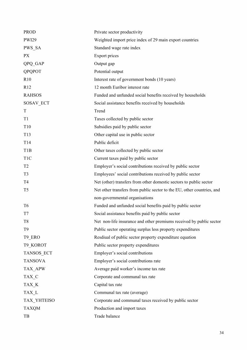
PROD Private sector productivity

PWI29 Weighted import price index of 29 main export countries

PWS_SA Standard wage rate index

PX Export prices

QPQ_GAP Output gap

QPQPOT Potential output

R10 Interest rate of government bonds (10 years)

R12 12 month Euribor interest rate

RAHSOS Funded and unfunded social benefits received by households

SOSAV_ECT Social assistance benefits received by households

T Trend

T1 Taxes collected by public sector

T10 Subsidies paid by public sector

T13 Other capital use in public sector

T14 Public deficit

T1B Other taxes collected by public sector

T1C Current taxes paid by public sector

T2 Employer’s social contributions received by public sector

T3 Employees’ social contributions received by public sector

T4 Net (other) transfers from other domestic sectors to public sector

T5 Net other transfers from public sector to the EU, other countries, and

non-governmental organisations

T6 Funded and unfunded social benefits paid by public sector

T7 Social assistance benefits paid by public sector

T8 Net non-life insurance and other premiums received by public sector

T9 Public sector operating surplus less property expenditures

T9_ERO Resdiual of public sector property expenditure equation

T9_KOROT Public sector property expenditures

TANSOS_ECT Employer’s social contributions

TANSOVA Employer’s social contributions rate

TAX_APW Average paid worker’s income tax rate

TAX_C Corporate and communal tax rate

TAX_K Capital tax rate

TAX_L Communal tax rate (average)

TAX_YHTEISO Corporate and communal taxes received by public sector

TAXQM Production and import taxes

TB Trade balance

35

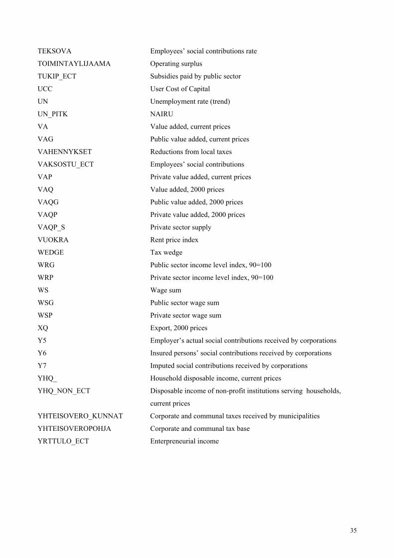
TEKSOVA Employees’ social contributions rate

TOIMINTAYLIJAAMA Operating surplus

TUKIP_ECT Subsidies paid by public sector

UCC User Cost of Capital

UN Unemployment rate (trend)

UN_PITK NAIRU

VA Value added, current prices

VAG Public value added, current prices

VAHENNYKSET Reductions from local taxes

VAKSOSTU_ECT Employees’ social contributions

VAP Private value added, current prices

VAQ Value added, 2000 prices

VAQG Public value added, 2000 prices

VAQP Private value added, 2000 prices

VAQP_S Private sector supply

VUOKRA Rent price index

WEDGE Tax wedge

WRG Public sector income level index, 90=100

WRP Private sector income level index, 90=100

WS Wage sum

WSG Public sector wage sum

WSP Private sector wage sum

XQ Export, 2000 prices

Y5 Employer’s actual social contributions received by corporations

Y6 Insured persons’ social contributions received by corporations

Y7 Imputed social contributions received by corporations

YHQ_ Household disposable income, current prices

YHQ_NON_ECT Disposable income of non-profit institutions serving households,

current prices

YHTEISOVERO_KUNNAT Corporate and communal taxes received by municipalities

YHTEISOVEROPOHJA Corporate and communal tax base

YRTTULO_ECT Enterpreneurial income

36

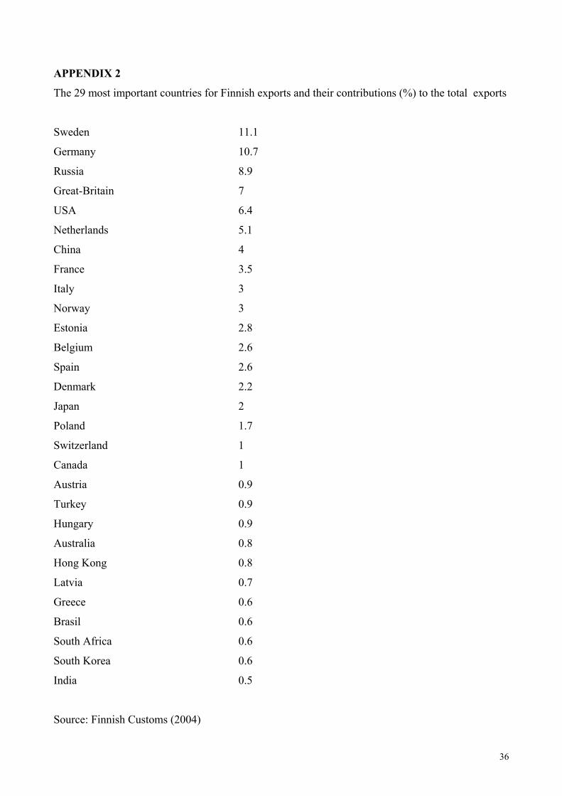
APPENDIX 2

The 29 most important countries for Finnish exports and their contributions (%) to the total exports

Sweden 11.1

Germany 10.7

Russia 8.9

Great-Britain 7

USA 6.4

Netherlands 5.1

China 4

France 3.5

Italy 3

Norway 3

Estonia 2.8

Belgium 2.6

Spain 2.6

Denmark 2.2

Japan 2

Poland 1.7

Switzerland 1

Canada 1

Austria 0.9

Turkey 0.9

Hungary 0.9

Australia 0.8

Hong Kong 0.8

Latvia 0.7

Greece 0.6

Brasil 0.6

South Africa 0.6

South Korea 0.6

India 0.5

Source: Finnish Customs (2004)

37

References

Chirinko, R. S. (1993): Business Fixed Investment Spending: Modeling Strategies, Empirical

Results, and Policy Implications. Journal of Economic Literature, Vol 31, No. 4, 1875–1911.

Engle, R. F. & Granger, C. W. J. (1987): Co-integration and Error Correction: Representation,

Estimation, and Testing. Econometrica, Vol. 55, No. 2, 251–276.

Gabriel, F., Henry, J. & Mestre, R. (2001): An Area-wide Model for the Euro Area. European

Central Bank Working Paper Series, Working Paper No. 42.

Gómez, V. & Maravall A. (1997): Programs TRAMO and SEATS. Instructions for the User.

Manual.

Hall, S. G. & Henry S. G. B (1989): Macroeconomic modelling. 2. edition. Amsterdam: North-

Holland.

Kiander, J. , Vilmunen, J. & Virén, M. (2005): Miksi työ ei käy kaupaksi? Analyysejä VATT:n

yrityspaneeliaineistolla 1994–2002.

Lehmus, M. (2006): Suomen talouden ennustemallin rakentaminen. Pro Gradu thesis, University of

Turku.

Mayes, D. & Virén, M. (2002): Financial Condition Indices. International Economics LV:4, 521–

550.

Phillips, A. W. (1958): The Relation between Unemployment and the Rate of Change of Money

Wage Rates in the United Kingdom, 1861–1957, Economica, NS. 25, no. 2, 283–299.

Szeto, K. L. (2001): An Econometric Analysis of a Production Function for New Zealand.

Treasury Working Paper, 01/31.

Tinbergen, J. (1939): Business Cycles in the United States: 1912–1932. League of Nations.

38

Valadkhani, A. (2004): History of Macroeconometric modelling: lessons from past experience.

Journal of Policy Modeling, 26, 266–281.

Virén, M. & Pachucki, D. & Dudek, S. (2003): Quarterly Public Finance Sector Model of the

Polish Ministry of Finance, non-published manuscript.