Embed Size (px)
Citation preview
Using ML for Propensity Scores Propensity score: Pr | Propensity score weighting and matching is common in
treatment effects literature “Selection on observables assumption”: | See Imbens and Rubin (2015) for extensive review
Propensity score estimation is a pure prediction problem Machine learning literature applies propensity score weighting: e.g.
Beygelzimer and Langford (2009), Dudick, Langford and Li (2011) Properties or tradeoffs in selection among ML approaches
Estimated propensity scores work better than true propensity score (Hirano, Imbens and Ridder (2003)), so optimizing for out of sample prediction is not the best path
Various papers consider tradeoffs, no clear answer, but classification trees and random forests do well
Using ML for Model Specification under Selection on Observables
A heuristic: If you control richly for covariates, can estimate
treatment effect ignoring endogeneity This motivates regressions with rich specification
Naïve approach motivated by heuristic using LASSO Keep the treatment variable out of the model
selection by not penalizing it Use LASSO to select the rest of the model
specification Problem:
Treatment variable is forced in, and some covariates will have coefficients forced to zero.
Treatment effect coefficient will pick up those effects and will thus be biased.
See Belloni, Chernozhukov and Hansen JEP 2014 for an accessible discussion of this
Better approach: Need to do variable
selection via LASSO for the selection equation and outcome equation separately
Use LASSO with the union of variables selected
Belloni, Chernozhukov & Hansen (2013) show that this works under some assumptions, including constant treatment effects
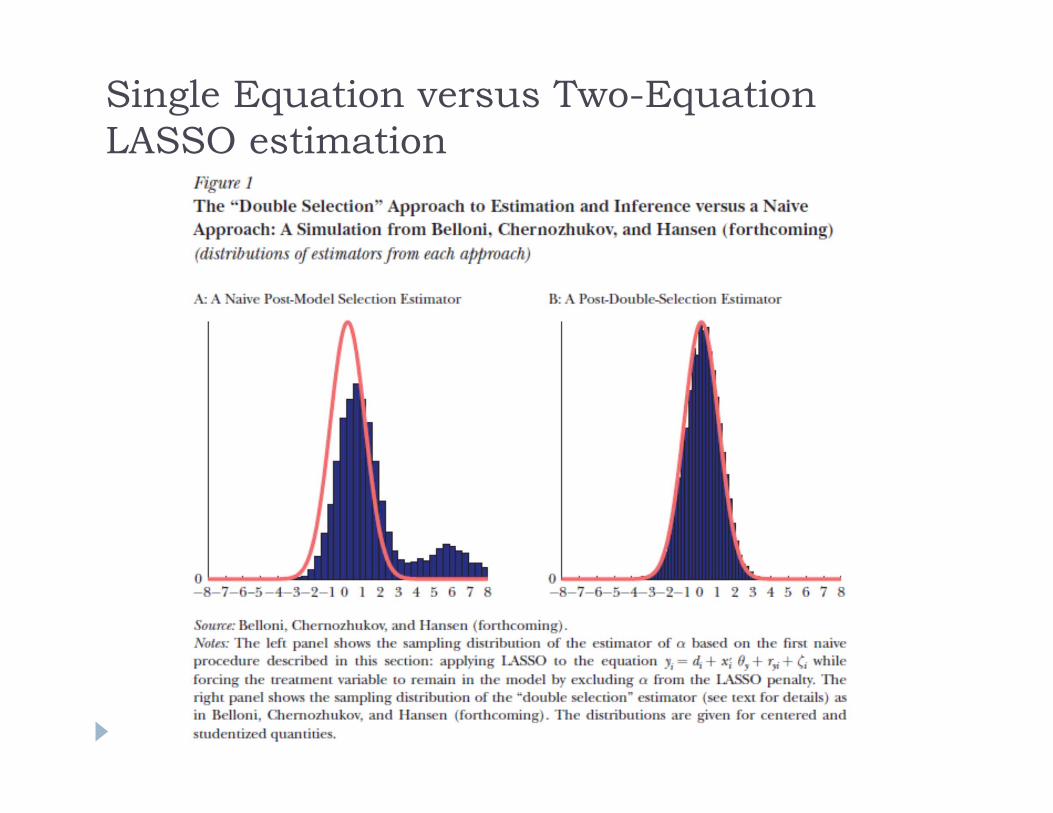
Single Equation versus Two-Equation LASSO estimation
Using ML for the first stage of IV IV assumptions | See Imbens and Rubin (2015) for extensive review
First stage estimation: instrument selection and functional form | , This is a prediction problem where
interpretability is less important Variety of methods available Belloni, Chernozhukov, and Hansen (2010); Belloni, Chen,
Chernozhukov and Hansen (2012) proposed LASSO Under some conditions, second stage inference occurs as usual Key: second-stage is immune to misspecification in the first stage
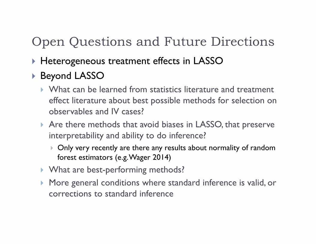
Open Questions and Future Directions Heterogeneous treatment effects in LASSO Beyond LASSO What can be learned from statistics literature and treatment
effect literature about best possible methods for selection on observables and IV cases?
Are there methods that avoid biases in LASSO, that preserve interpretability and ability to do inference? Only very recently are there any results about normality of random
forest estimators (e.g. Wager 2014)
What are best-performing methods? More general conditions where standard inference is valid, or
corrections to standard inference

Machine Learning Methods for Estimating Heterogeneous Causal
Effects
Athey and Imbens, 2015http://arxiv.org/abs/1504.01132
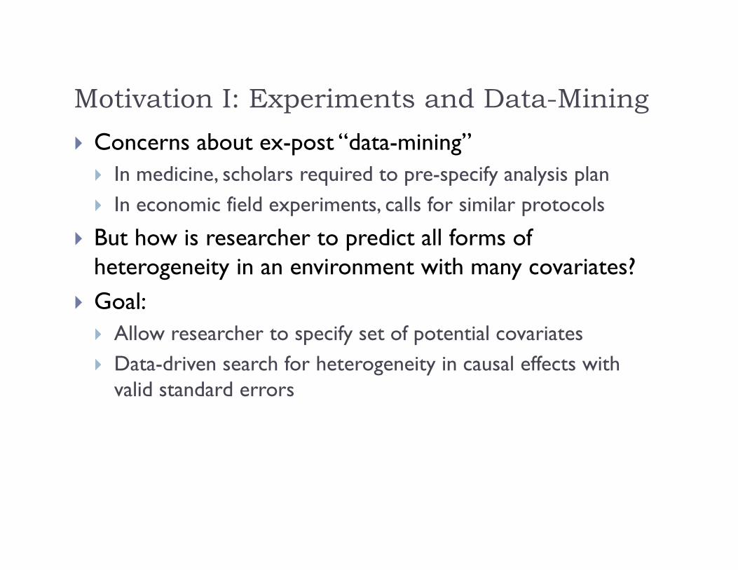
Motivation I: Experiments and Data-Mining Concerns about ex-post “data-mining” In medicine, scholars required to pre-specify analysis plan In economic field experiments, calls for similar protocols
But how is researcher to predict all forms of heterogeneity in an environment with many covariates?
Goal: Allow researcher to specify set of potential covariates Data-driven search for heterogeneity in causal effects with
valid standard errors
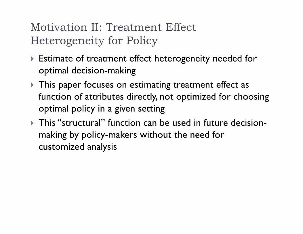
Motivation II: Treatment Effect Heterogeneity for Policy Estimate of treatment effect heterogeneity needed for
optimal decision-making This paper focuses on estimating treatment effect as
function of attributes directly, not optimized for choosing optimal policy in a given setting
This “structural” function can be used in future decision-making by policy-makers without the need for customized analysis
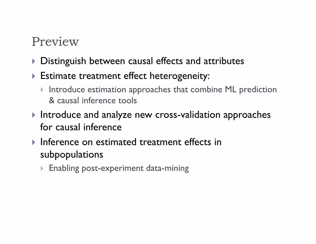
Preview Distinguish between causal effects and attributes Estimate treatment effect heterogeneity: Introduce estimation approaches that combine ML prediction
& causal inference tools
Introduce and analyze new cross-validation approaches for causal inference
Inference on estimated treatment effects in subpopulations Enabling post-experiment data-mining
Regression Trees for Prediction
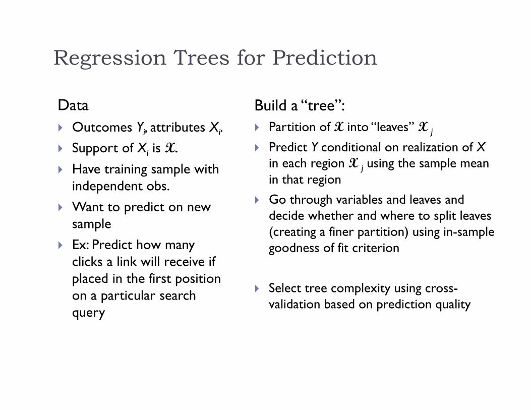
Data Outcomes Yi, attributes Xi. Support of Xi is X. Have training sample with
independent obs. Want to predict on new
sample Ex: Predict how many
clicks a link will receive if placed in the first position on a particular search query
Build a “tree”: Partition of X into “leaves” X j Predict Y conditional on realization of X
in each region X j using the sample mean in that region
Go through variables and leaves and decide whether and where to split leaves (creating a finer partition) using in-sample goodness of fit criterion
Select tree complexity using cross-validation based on prediction quality
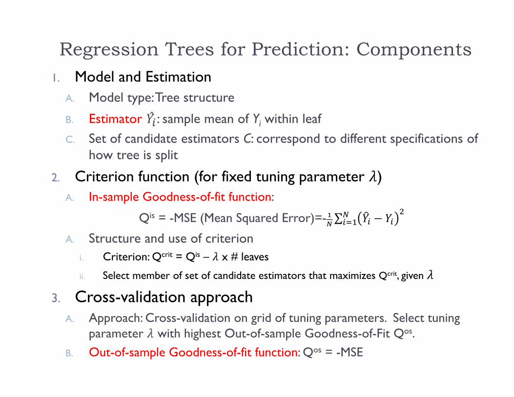
Regression Trees for Prediction: Components1. Model and Estimation
A. Model type: Tree structure
B. Estimator : sample mean of Yi within leafC. Set of candidate estimators C: correspond to different specifications of
how tree is split
2. Criterion function (for fixed tuning parameter )A. In-sample Goodness-of-fit function:
Qis = -MSE (Mean Squared Error)=- ∑
A. Structure and use of criterioni. Criterion: Qcrit = Qis – x # leaves
ii. Select member of set of candidate estimators that maximizes Qcrit, given
3. Cross-validation approachA. Approach: Cross-validation on grid of tuning parameters. Select tuning
parameter with highest Out-of-sample Goodness-of-Fit Qos.B. Out-of-sample Goodness-of-fit function: Qos = -MSE
Using Trees to Estimate Causal Effects
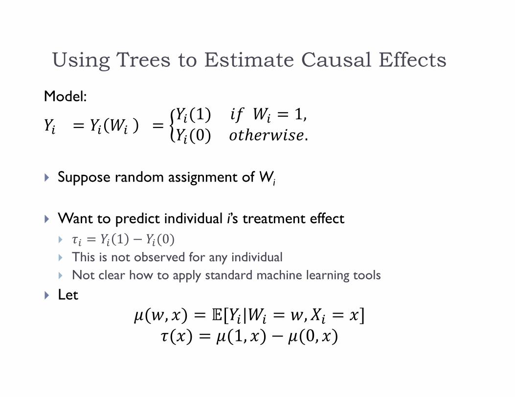
Model:
Suppose random assignment of Wi
Want to predict individual i’s treatment effect 1 0 This is not observed for any individual Not clear how to apply standard machine learning tools
Let
Using Trees to Estimate Causal Effects, | ,
1, 0,
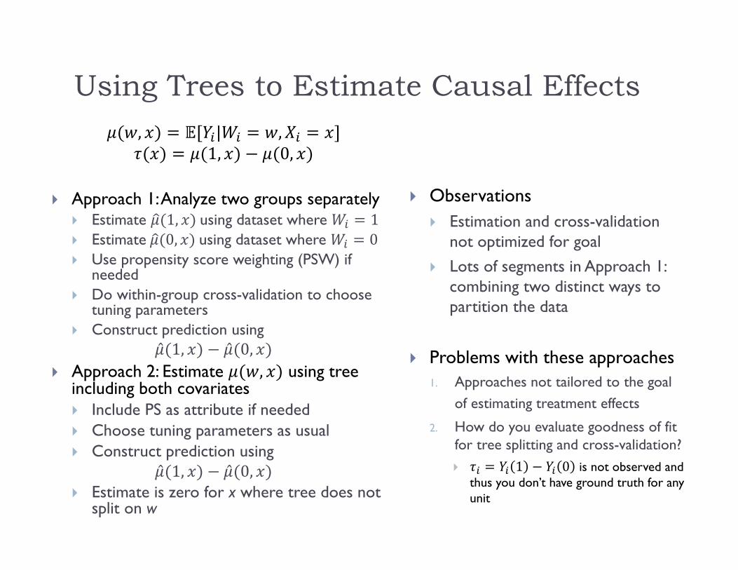
Approach 1: Analyze two groups separately Estimate 1, using dataset where 1 Estimate 0, using dataset where 0 Use propensity score weighting (PSW) if
needed Do within-group cross-validation to choose
tuning parameters Construct prediction using
1, 0, Approach 2: Estimate , using tree
including both covariates Include PS as attribute if needed Choose tuning parameters as usual Construct prediction using
1, 0, Estimate is zero for x where tree does not
split on w
Observations Estimation and cross-validation
not optimized for goal Lots of segments in Approach 1:
combining two distinct ways to partition the data
Problems with these approaches1. Approaches not tailored to the goal
of estimating treatment effects
2. How do you evaluate goodness of fit for tree splitting and cross-validation? 1 0 is not observed and
thus you don’t have ground truth for any unit
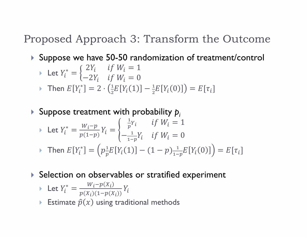
Proposed Approach 3: Transform the Outcome
Suppose we have 50-50 randomization of treatment/control
Let ∗ 2 12 0
Then ∗ 2 ⋅ 1 0
Suppose treatment with probability pi
Let ∗ 1 0
Then ∗ 1 1 0
Selection on observables or stratified experiment Let ∗
Estimate using traditional methods
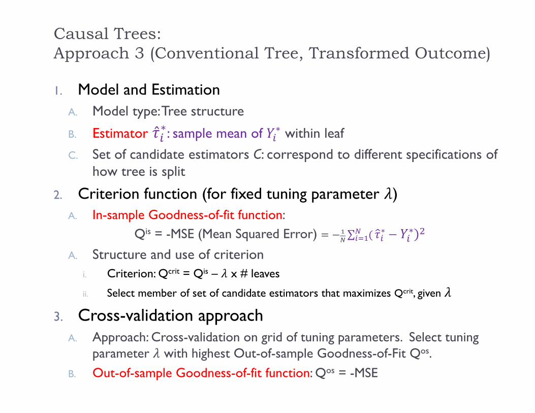
Causal Trees: Approach 3 (Conventional Tree, Transformed Outcome)
1. Model and EstimationA. Model type: Tree structure
B. Estimator ∗: sample mean of ∗ within leafC. Set of candidate estimators C: correspond to different specifications of
how tree is split
2. Criterion function (for fixed tuning parameter )A. In-sample Goodness-of-fit function:
Qis = -MSE (Mean Squared Error) ∑ ∗ ∗ A. Structure and use of criterion
i. Criterion: Qcrit = Qis – x # leaves
ii. Select member of set of candidate estimators that maximizes Qcrit, given
3. Cross-validation approachA. Approach: Cross-validation on grid of tuning parameters. Select tuning
parameter with highest Out-of-sample Goodness-of-Fit Qos.B. Out-of-sample Goodness-of-fit function: Qos = -MSE
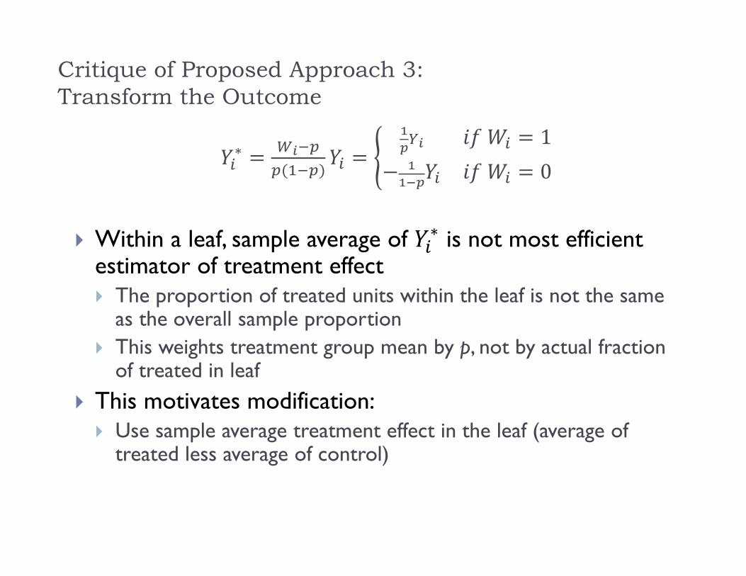
Critique of Proposed Approach 3: Transform the Outcome
∗ 1 0
Within a leaf, sample average of ∗ is not most efficient estimator of treatment effect The proportion of treated units within the leaf is not the same
as the overall sample proportion This weights treatment group mean by p, not by actual fraction
of treated in leaf This motivates modification: Use sample average treatment effect in the leaf (average of
treated less average of control)
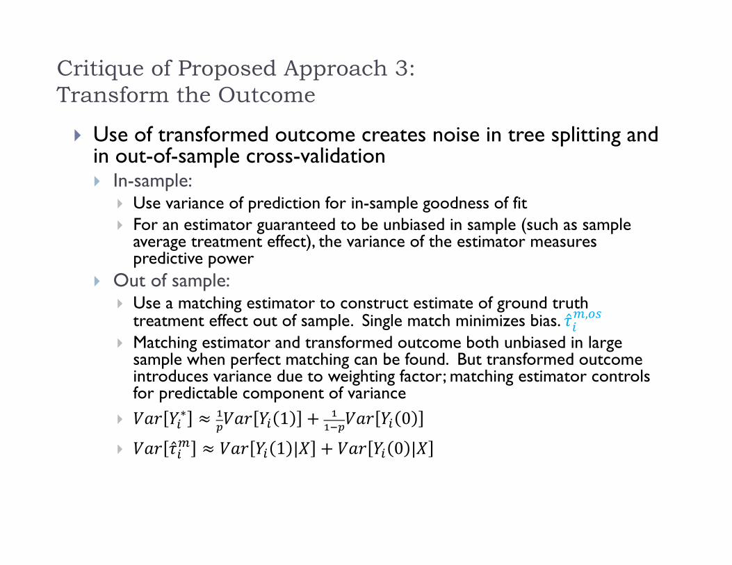
Critique of Proposed Approach 3: Transform the Outcome
Use of transformed outcome creates noise in tree splitting and in out-of-sample cross-validation In-sample:
Use variance of prediction for in-sample goodness of fit For an estimator guaranteed to be unbiased in sample (such as sample
average treatment effect), the variance of the estimator measures predictive power
Out of sample: Use a matching estimator to construct estimate of ground truth
treatment effect out of sample. Single match minimizes bias. ,
Matching estimator and transformed outcome both unbiased in large sample when perfect matching can be found. But transformed outcome introduces variance due to weighting factor; matching estimator controls for predictable component of variance
∗ 1 0
1 | 0 |
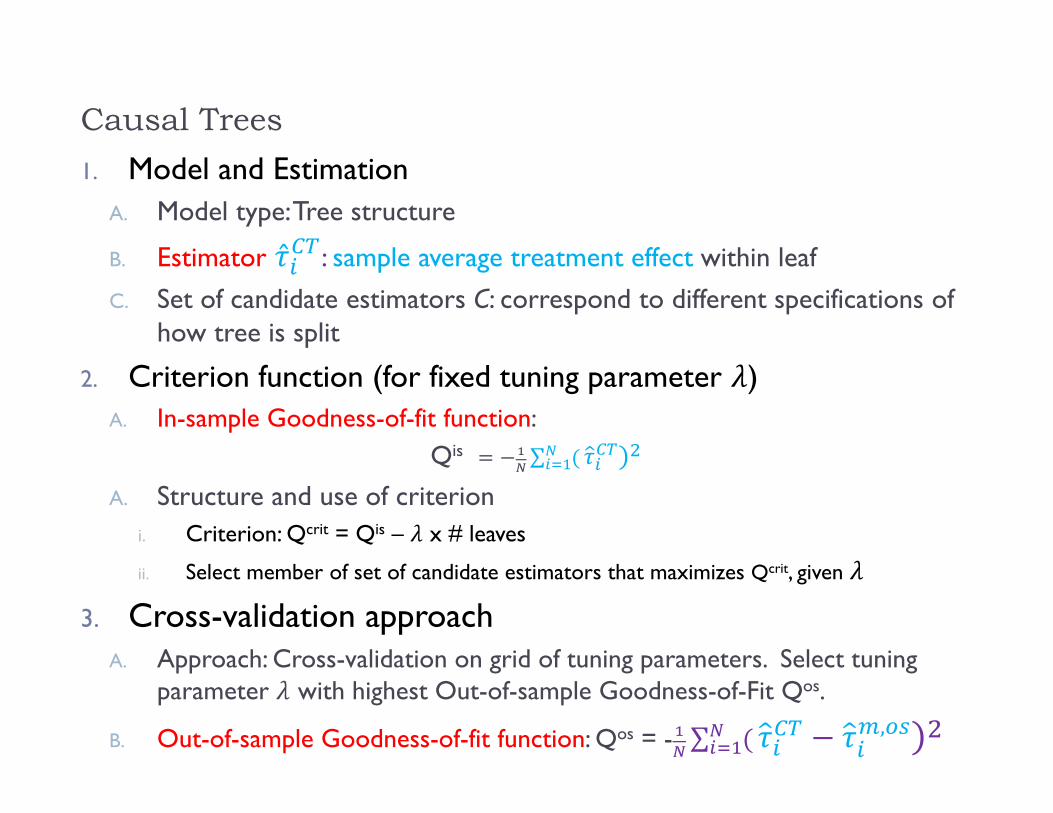
Causal Trees1. Model and Estimation
A. Model type: Tree structure
B. Estimator : sample average treatment effect within leafC. Set of candidate estimators C: correspond to different specifications of
how tree is split
2. Criterion function (for fixed tuning parameter )A. In-sample Goodness-of-fit function:
Qis ∑ A. Structure and use of criterion
i. Criterion: Qcrit = Qis – x # leaves
ii. Select member of set of candidate estimators that maximizes Qcrit, given
3. Cross-validation approachA. Approach: Cross-validation on grid of tuning parameters. Select tuning
parameter with highest Out-of-sample Goodness-of-Fit Qos.
B. Out-of-sample Goodness-of-fit function: Qos = - ∑ ,
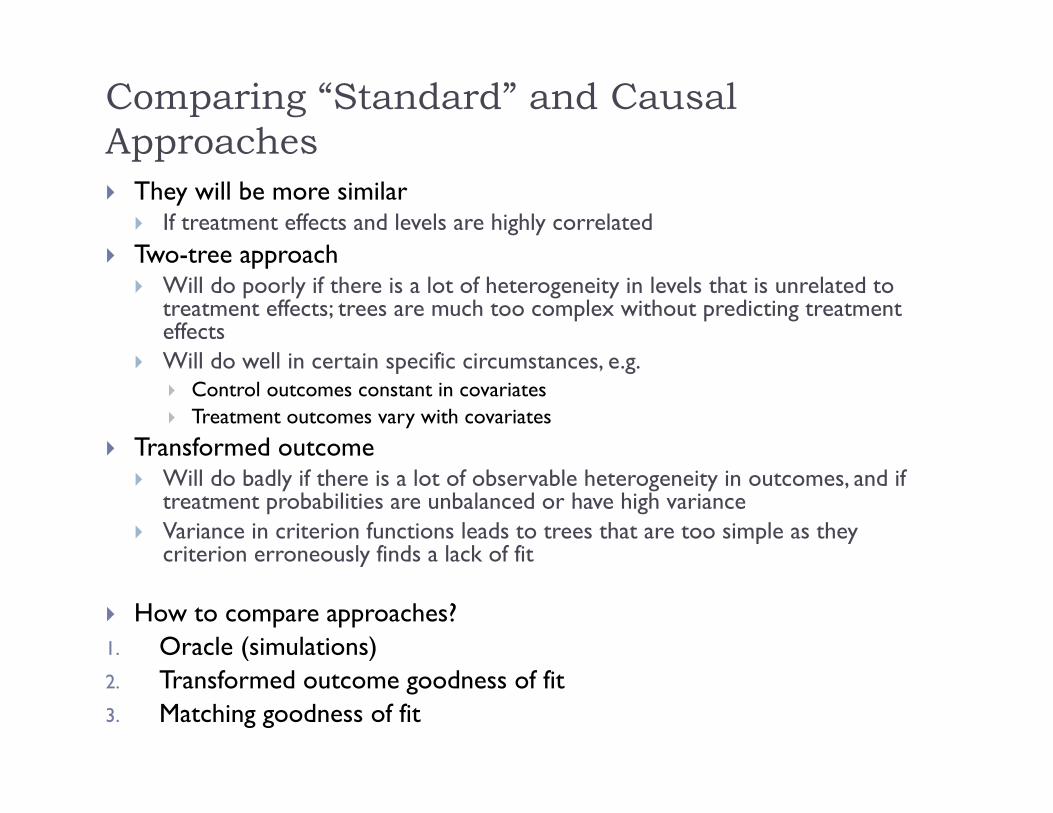
Comparing “Standard” and Causal Approaches They will be more similar
If treatment effects and levels are highly correlated Two-tree approach
Will do poorly if there is a lot of heterogeneity in levels that is unrelated to treatment effects; trees are much too complex without predicting treatment effects
Will do well in certain specific circumstances, e.g. Control outcomes constant in covariates Treatment outcomes vary with covariates
Transformed outcome Will do badly if there is a lot of observable heterogeneity in outcomes, and if
treatment probabilities are unbalanced or have high variance Variance in criterion functions leads to trees that are too simple as they
criterion erroneously finds a lack of fit
How to compare approaches?1. Oracle (simulations)2. Transformed outcome goodness of fit3. Matching goodness of fit
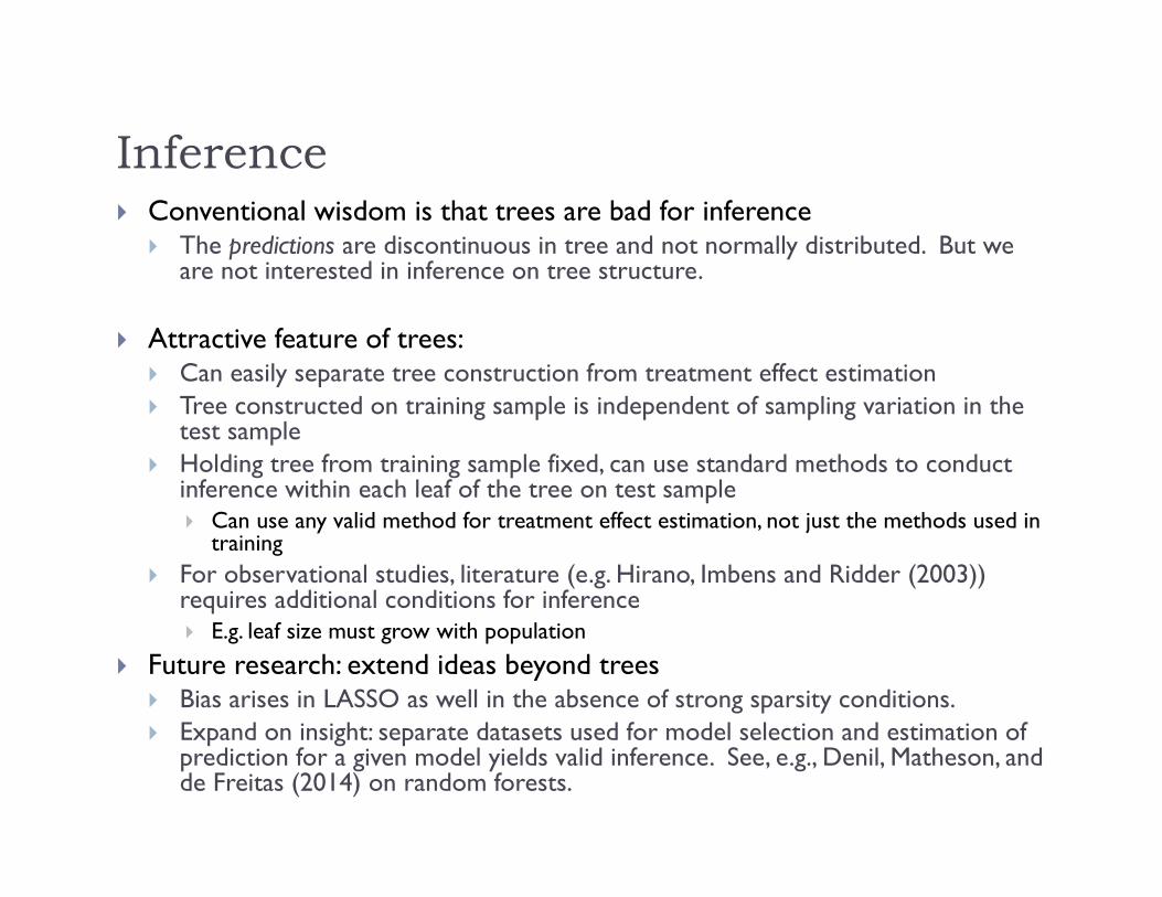
Inference Conventional wisdom is that trees are bad for inference
The predictions are discontinuous in tree and not normally distributed. But we are not interested in inference on tree structure.
Attractive feature of trees: Can easily separate tree construction from treatment effect estimation Tree constructed on training sample is independent of sampling variation in the
test sample Holding tree from training sample fixed, can use standard methods to conduct
inference within each leaf of the tree on test sample Can use any valid method for treatment effect estimation, not just the methods used in
training For observational studies, literature (e.g. Hirano, Imbens and Ridder (2003))
requires additional conditions for inference E.g. leaf size must grow with population
Future research: extend ideas beyond trees Bias arises in LASSO as well in the absence of strong sparsity conditions. Expand on insight: separate datasets used for model selection and estimation of
prediction for a given model yields valid inference. See, e.g., Denil, Matheson, and de Freitas (2014) on random forests.
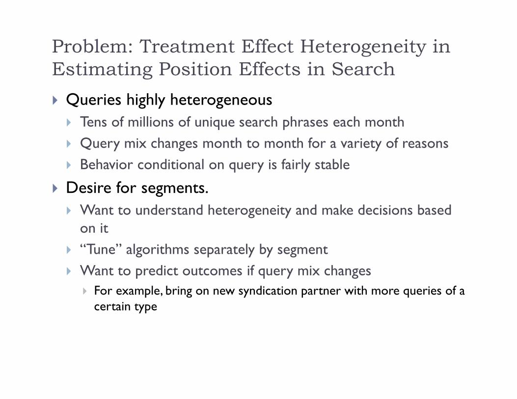
Problem: Treatment Effect Heterogeneity in Estimating Position Effects in Search Queries highly heterogeneous Tens of millions of unique search phrases each month Query mix changes month to month for a variety of reasons Behavior conditional on query is fairly stable
Desire for segments. Want to understand heterogeneity and make decisions based
on it “Tune” algorithms separately by segment Want to predict outcomes if query mix changes
For example, bring on new syndication partner with more queries of a certain type
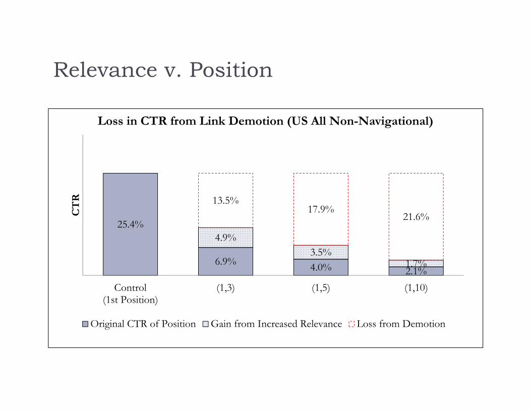
Relevance v. Position
25.4%
6.9% 4.0% 2.1%
4.9%3.5%
1.7%
13.5%17.9%
21.6%
Control(1st Position)
(1,3) (1,5) (1,10)
CT
R
Loss in CTR from Link Demotion (US All Non-Navigational)
Original CTR of Position Gain from Increased Relevance Loss from Demotion
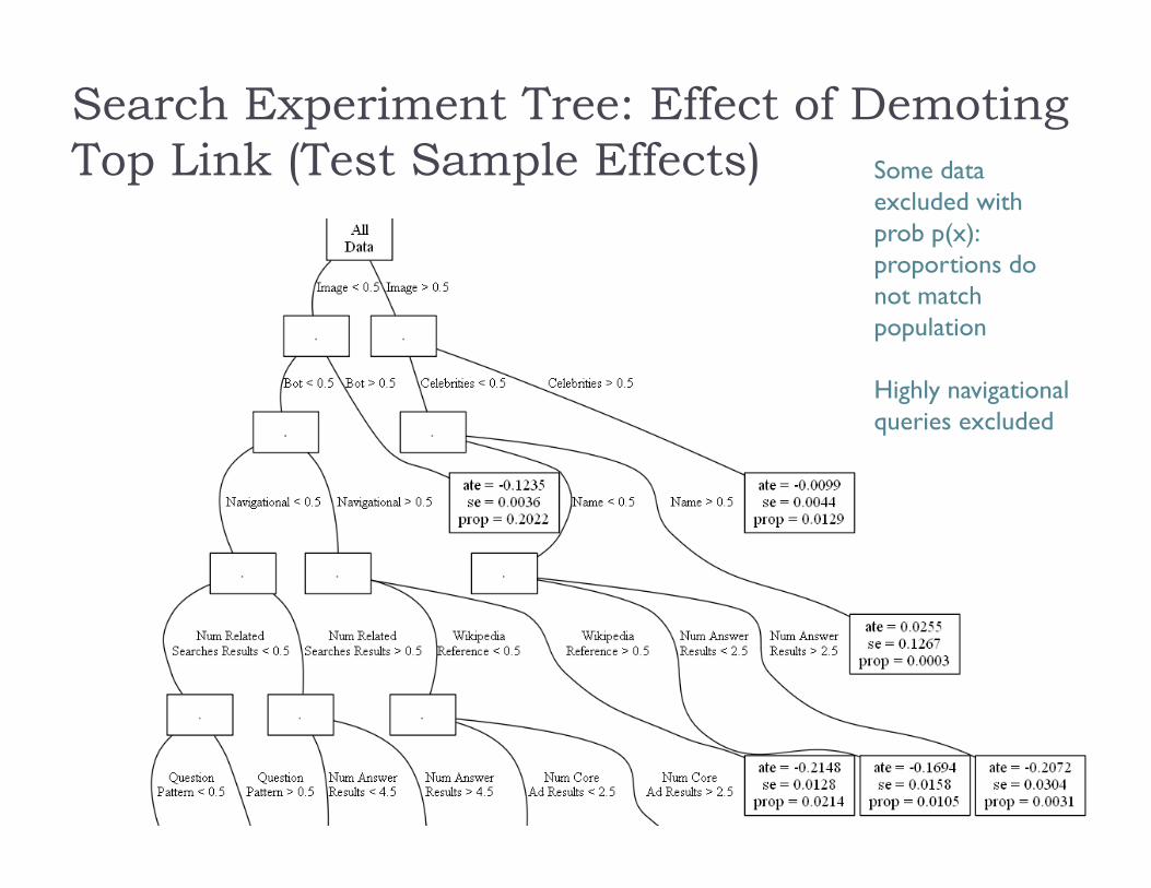
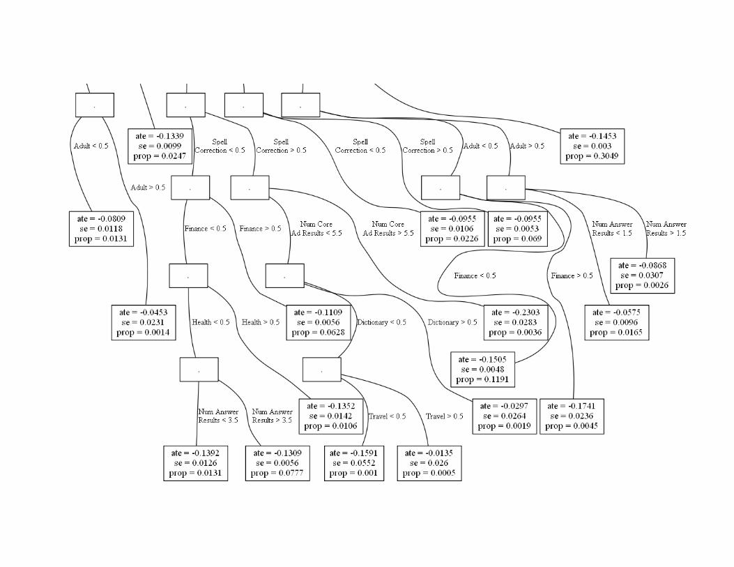
Search Experiment Tree: Effect of Demoting Top Link (Test Sample Effects) Some data
excluded with prob p(x): proportions do not match population
Highly navigational queries excluded
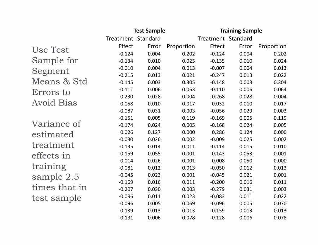
Use Test Sample for Segment Means & StdErrors to Avoid Bias
Variance of estimated treatment effects in training sample 2.5 times that in test sample
Test Sample Training SampleTreatment
EffectStandard
Error ProportionTreatment
EffectStandard
Error Proportion‐0.124 0.004 0.202 ‐0.124 0.004 0.202‐0.134 0.010 0.025 ‐0.135 0.010 0.024‐0.010 0.004 0.013 ‐0.007 0.004 0.013‐0.215 0.013 0.021 ‐0.247 0.013 0.022‐0.145 0.003 0.305 ‐0.148 0.003 0.304‐0.111 0.006 0.063 ‐0.110 0.006 0.064‐0.230 0.028 0.004 ‐0.268 0.028 0.004‐0.058 0.010 0.017 ‐0.032 0.010 0.017‐0.087 0.031 0.003 ‐0.056 0.029 0.003‐0.151 0.005 0.119 ‐0.169 0.005 0.119‐0.174 0.024 0.005 ‐0.168 0.024 0.0050.026 0.127 0.000 0.286 0.124 0.000‐0.030 0.026 0.002 ‐0.009 0.025 0.002‐0.135 0.014 0.011 ‐0.114 0.015 0.010‐0.159 0.055 0.001 ‐0.143 0.053 0.001‐0.014 0.026 0.001 0.008 0.050 0.000‐0.081 0.012 0.013 ‐0.050 0.012 0.013‐0.045 0.023 0.001 ‐0.045 0.021 0.001‐0.169 0.016 0.011 ‐0.200 0.016 0.011‐0.207 0.030 0.003 ‐0.279 0.031 0.003‐0.096 0.011 0.023 ‐0.083 0.011 0.022‐0.096 0.005 0.069 ‐0.096 0.005 0.070‐0.139 0.013 0.013 ‐0.159 0.013 0.013‐0.131 0.006 0.078 ‐0.128 0.006 0.078
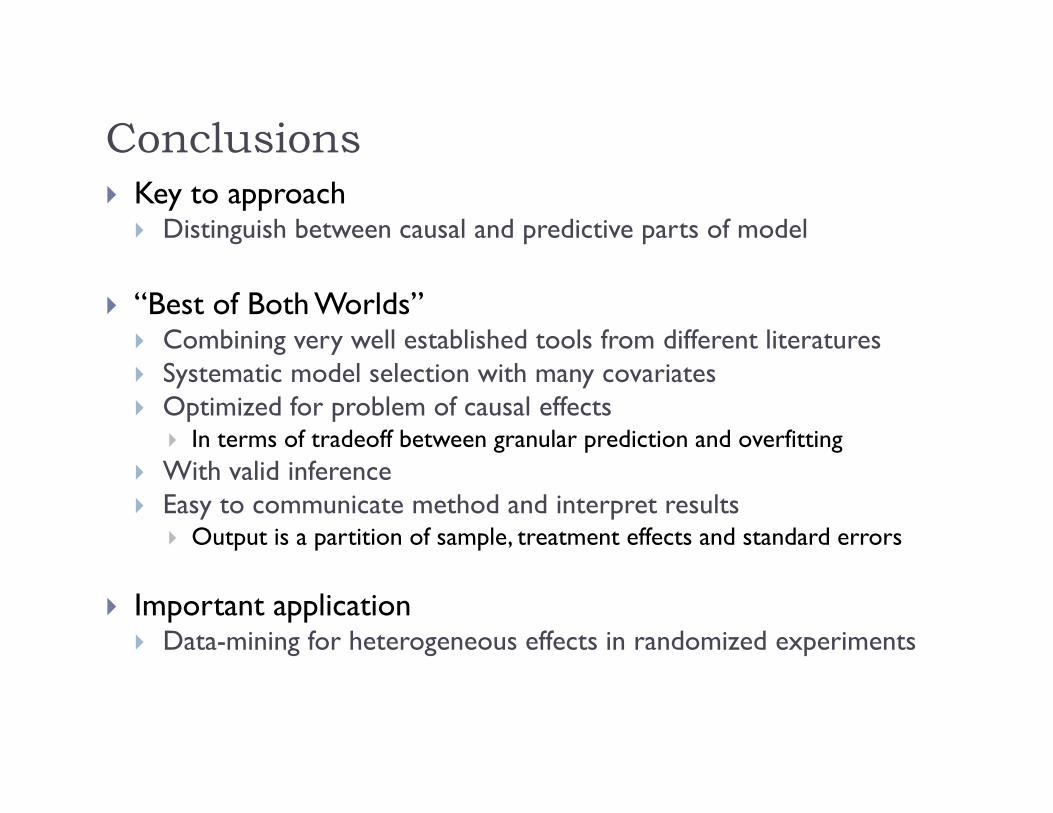
Conclusions Key to approach Distinguish between causal and predictive parts of model
“Best of Both Worlds” Combining very well established tools from different literatures Systematic model selection with many covariates Optimized for problem of causal effects
In terms of tradeoff between granular prediction and overfitting With valid inference Easy to communicate method and interpret results
Output is a partition of sample, treatment effects and standard errors
Important application Data-mining for heterogeneous effects in randomized experiments
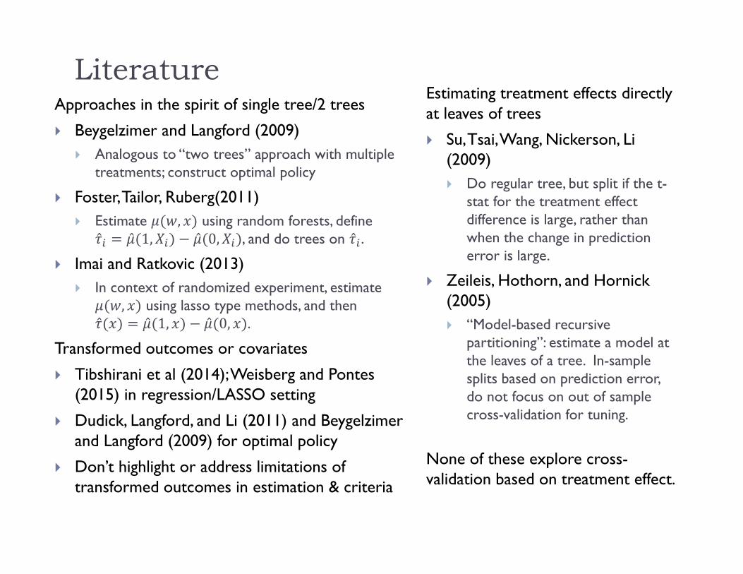
LiteratureApproaches in the spirit of single tree/2 trees
Beygelzimer and Langford (2009) Analogous to “two trees” approach with multiple
treatments; construct optimal policy
Foster, Tailor, Ruberg(2011) Estimate , using random forests, define
1, 0, , and do trees on .
Imai and Ratkovic (2013) In context of randomized experiment, estimate
, using lasso type methods, and then 1, 0, .
Transformed outcomes or covariates
Tibshirani et al (2014); Weisberg and Pontes (2015) in regression/LASSO setting
Dudick, Langford, and Li (2011) and Beygelzimerand Langford (2009) for optimal policy
Don’t highlight or address limitations of transformed outcomes in estimation & criteria
Estimating treatment effects directly at leaves of trees
Su, Tsai, Wang, Nickerson, Li(2009) Do regular tree, but split if the t-
stat for the treatment effect difference is large, rather than when the change in prediction error is large.
Zeileis, Hothorn, and Hornick (2005) “Model-based recursive
partitioning”: estimate a model at the leaves of a tree. In-sample splits based on prediction error, do not focus on out of sample cross-validation for tuning.
None of these explore cross-validation based on treatment effect.
Extensions (Work in Progress) Alternatives for cross-validation criteria Optimizing selection on observables case What is the best way to estimate propensity score for
this application? Alternatives to propensity score weighting
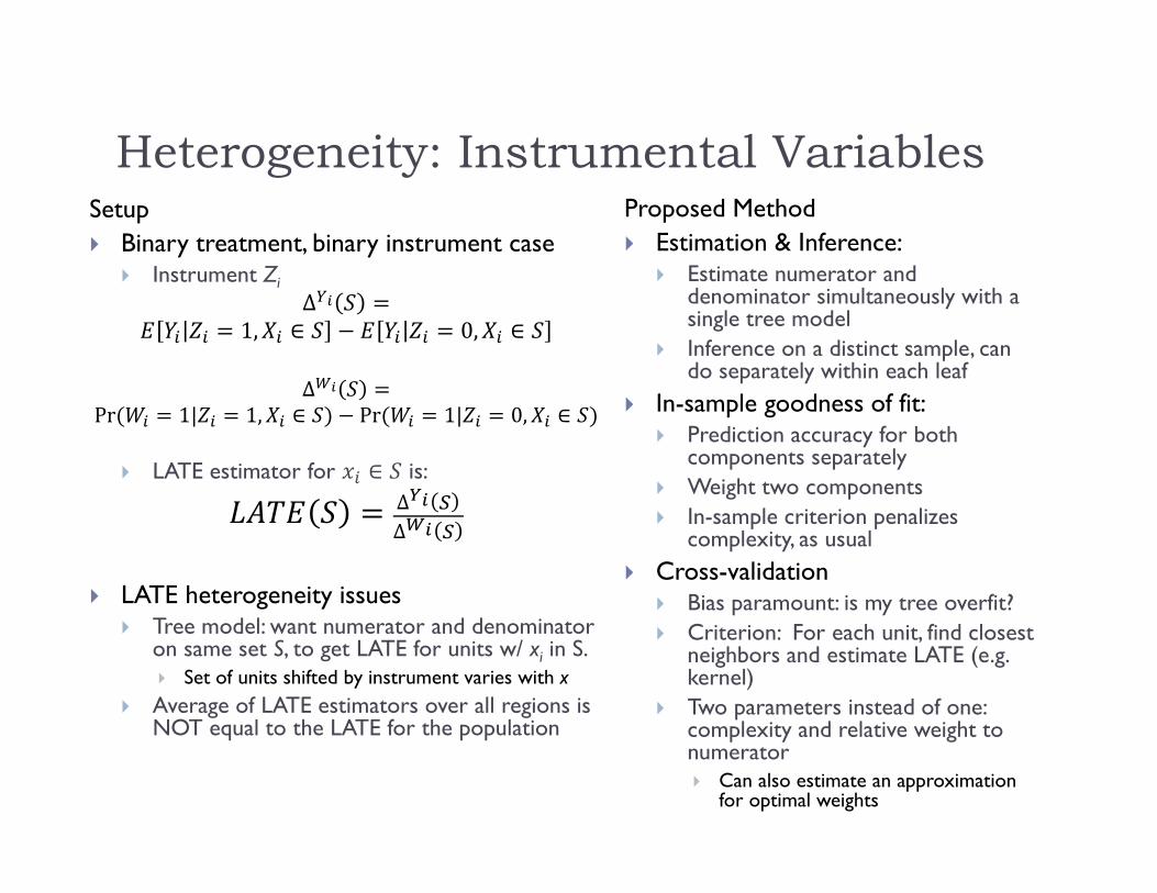
Heterogeneity: Instrumental VariablesSetup Binary treatment, binary instrument case
Instrument Zi∆
1, ∈ 0, ∈
∆Pr 1| 1, ∈ Pr 1| 0, ∈
LATE estimator for ∈ is:∆∆
LATE heterogeneity issues Tree model: want numerator and denominator
on same set S, to get LATE for units w/ xi in S. Set of units shifted by instrument varies with x
Average of LATE estimators over all regions is NOT equal to the LATE for the population
Proposed Method Estimation & Inference:
Estimate numerator and denominator simultaneously with a single tree model
Inference on a distinct sample, can do separately within each leaf
In-sample goodness of fit: Prediction accuracy for both
components separately Weight two components In-sample criterion penalizes
complexity, as usual Cross-validation
Bias paramount: is my tree overfit? Criterion: For each unit, find closest
neighbors and estimate LATE (e.g. kernel)
Two parameters instead of one: complexity and relative weight to numerator Can also estimate an approximation
for optimal weights
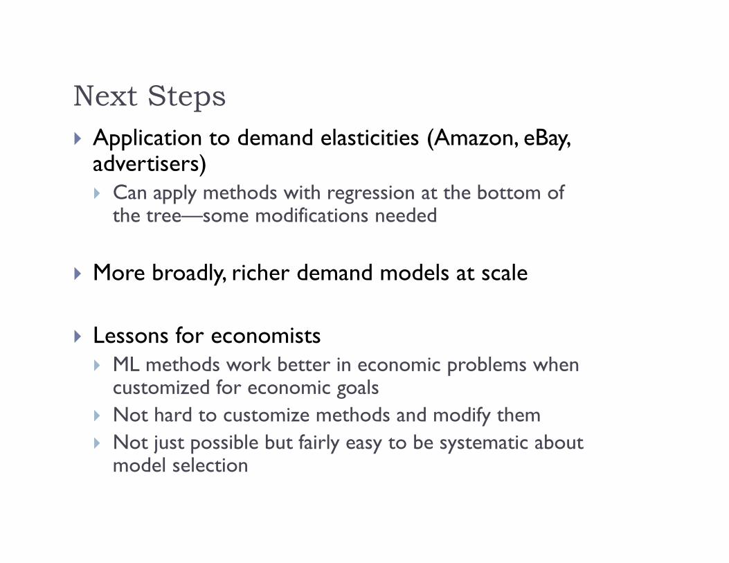
Next Steps Application to demand elasticities (Amazon, eBay,
advertisers) Can apply methods with regression at the bottom of
the tree—some modifications needed
More broadly, richer demand models at scale
Lessons for economists ML methods work better in economic problems when
customized for economic goals Not hard to customize methods and modify them Not just possible but fairly easy to be systematic about
model selection
Optimal Decision Rules as a Classification Problem
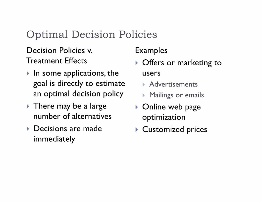
Optimal Decision PoliciesDecision Policies v. Treatment Effects In some applications, the
goal is directly to estimate an optimal decision policy
There may be a large number of alternatives
Decisions are made immediately
Examples Offers or marketing to
users Advertisements Mailings or emails
Online web page optimization
Customized prices
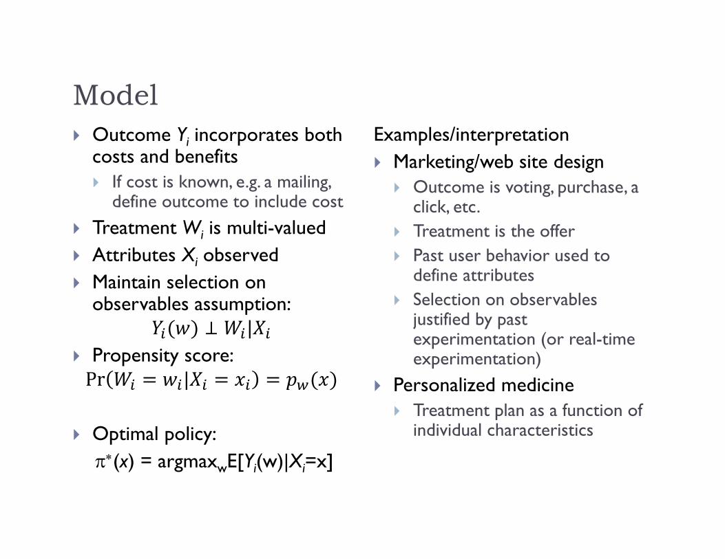
Model Outcome Yi incorporates both
costs and benefits If cost is known, e.g. a mailing,
define outcome to include cost Treatment Wi is multi-valued Attributes Xi observed Maintain selection on
observables assumption: |
Propensity score: Pr |
Optimal policy:(x) = argmaxwE[Yi(w)|Xi=x]
Examples/interpretation Marketing/web site design
Outcome is voting, purchase, a click, etc.
Treatment is the offer Past user behavior used to
define attributes Selection on observables
justified by past experimentation (or real-time experimentation)
Personalized medicine Treatment plan as a function of
individual characteristics
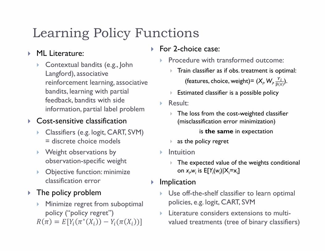
Learning Policy Functions ML Literature:
Contextual bandits (e.g., John Langford), associative reinforcement learning, associative bandits, learning with partial feedback, bandits with side information, partial label problem
Cost-sensitive classification Classifiers (e.g. logit, CART, SVM)
= discrete choice models Weight observations by
observation-specific weight Objective function: minimize
classification error
The policy problem Minimize regret from suboptimal
policy (“policy regret”) ∗
For 2-choice case: Procedure with transformed outcome:
Train classifier as if obs. treatment is optimal:
(features, choice, weight)= (Xi, Wi, ).
Estimated classifier is a possible policy
Result: The loss from the cost-weighted classifier
(misclassification error minimization)
is the same in expectation
as the policy regret
Intuition The expected value of the weights conditional
on xi,wi is E[Yi(wi)|Xi=xi]
Implication Use off-the-shelf classifier to learn optimal
policies, e.g. logit, CART, SVM Literature considers extensions to multi-
valued treatments (tree of binary classifiers)
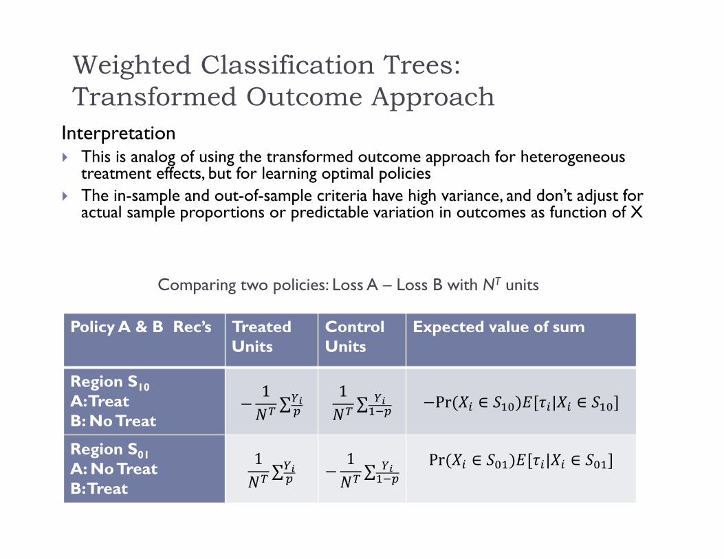
Weighted Classification Trees: Transformed Outcome Approach
Interpretation This is analog of using the transformed outcome approach for heterogeneous
treatment effects, but for learning optimal policies The in-sample and out-of-sample criteria have high variance, and don’t adjust for
actual sample proportions or predictable variation in outcomes as function of X
Comparing two policies: Loss A – Loss B with NT units
Policy A & B Rec’s Treated Units
Control Units
Expected value of sum
Region S10A: TreatB: No Treat
1∑
1∑ Pr ∈ | ∈
Region S01A: No TreatB: Treat
1∑
1∑
Pr ∈ | ∈
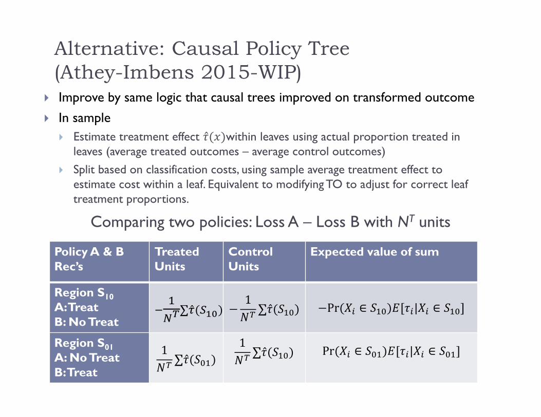
Alternative: Causal Policy Tree (Athey-Imbens 2015-WIP)
Improve by same logic that causal trees improved on transformed outcome
In sample Estimate treatment effect within leaves using actual proportion treated in
leaves (average treated outcomes – average control outcomes) Split based on classification costs, using sample average treatment effect to
estimate cost within a leaf. Equivalent to modifying TO to adjust for correct leaf treatment proportions.
Comparing two policies: Loss A – Loss B with NT units
Policy A & B Rec’s
Treated Units
Control Units
Expected value of sum
Region S10A: TreatB: No Treat
∑ 1∑ Pr ∈ | ∈
Region S01A: No TreatB: Treat
1∑
1∑ Pr ∈ | ∈
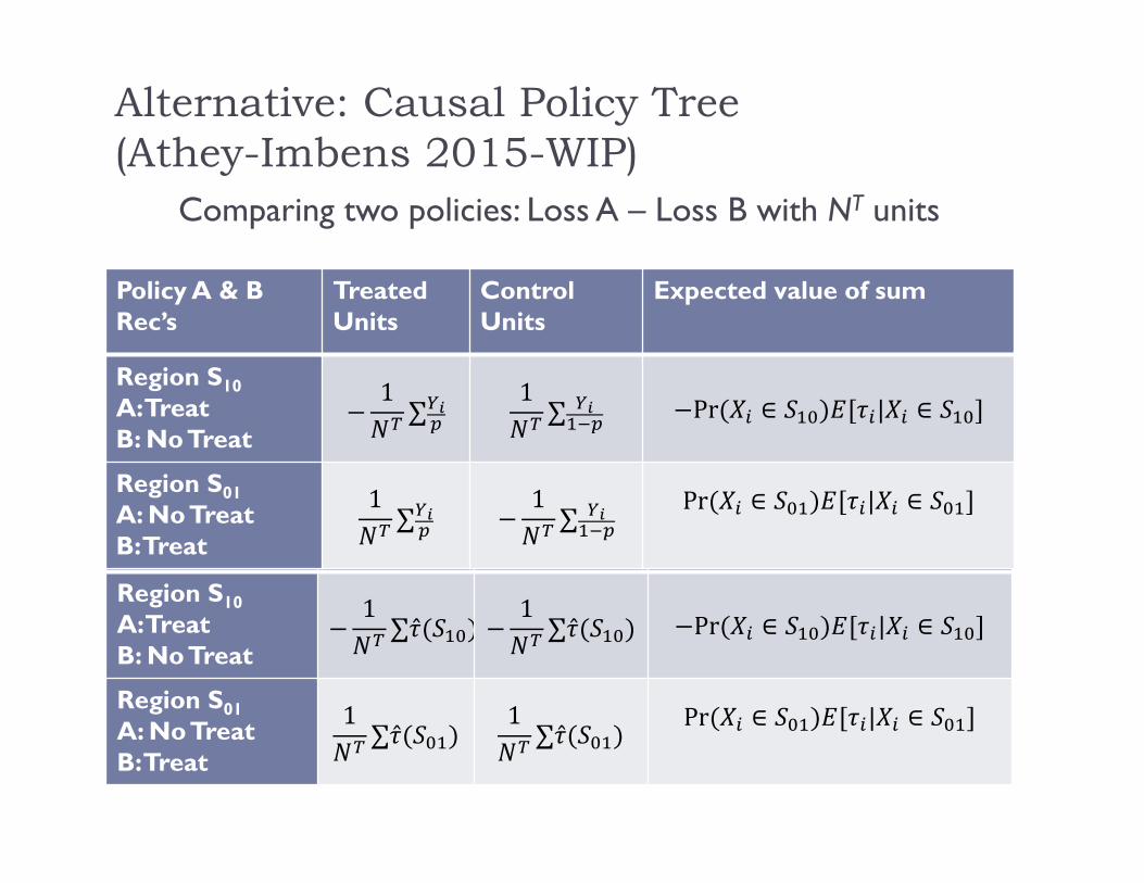
Alternative: Causal Policy Tree (Athey-Imbens 2015-WIP)
Comparing two policies: Loss A – Loss B with NT units
Policy A & B Rec’s
Treated Units
Control Units
Expected value of sum
Region S10A: TreatB: No Treat
1∑
1∑ Pr ∈ | ∈
Region S01A: No TreatB: Treat
1∑
1∑
Pr ∈ | ∈
Policy A & B Rec’s
Treated Units
Control Units
Expected value of sum
Region S10A: TreatB: No Treat
1∑
1∑ Pr ∈ | ∈
Region S01A: No TreatB: Treat
1∑
1∑
Pr ∈ | ∈
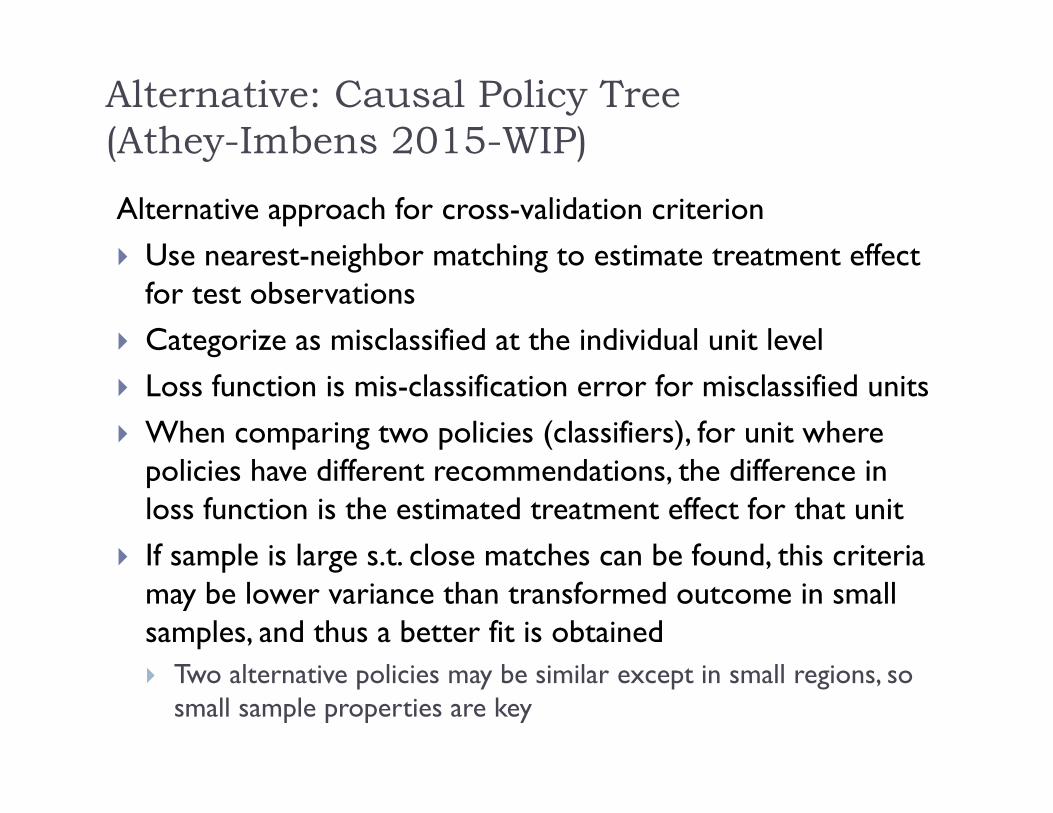
Alternative approach for cross-validation criterion Use nearest-neighbor matching to estimate treatment effect
for test observations Categorize as misclassified at the individual unit level Loss function is mis-classification error for misclassified units When comparing two policies (classifiers), for unit where
policies have different recommendations, the difference in loss function is the estimated treatment effect for that unit
If sample is large s.t. close matches can be found, this criteria may be lower variance than transformed outcome in small samples, and thus a better fit is obtained Two alternative policies may be similar except in small regions, so
small sample properties are key
Alternative: Causal Policy Tree (Athey-Imbens 2015-WIP)
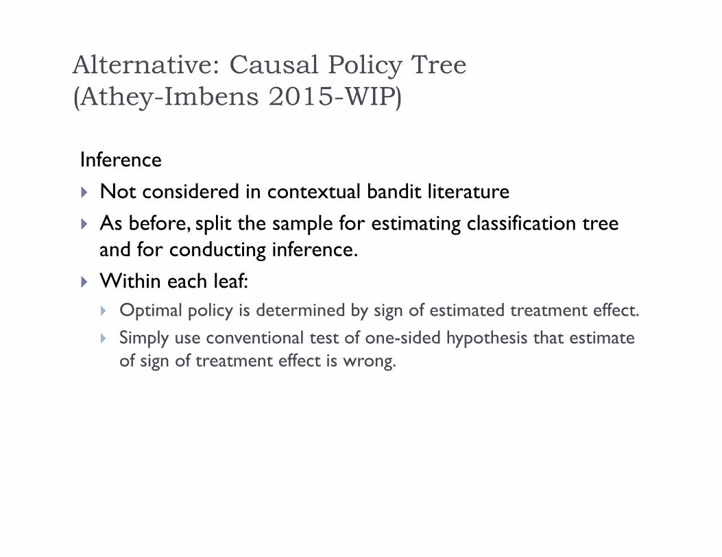
Inference Not considered in contextual bandit literature As before, split the sample for estimating classification tree
and for conducting inference. Within each leaf: Optimal policy is determined by sign of estimated treatment effect. Simply use conventional test of one-sided hypothesis that estimate
of sign of treatment effect is wrong.
Alternative: Causal Policy Tree (Athey-Imbens 2015-WIP)
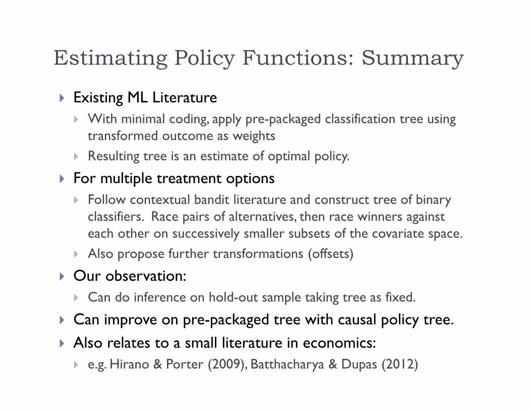
Existing ML Literature With minimal coding, apply pre-packaged classification tree using
transformed outcome as weights Resulting tree is an estimate of optimal policy.
For multiple treatment options Follow contextual bandit literature and construct tree of binary
classifiers. Race pairs of alternatives, then race winners against each other on successively smaller subsets of the covariate space.
Also propose further transformations (offsets)
Our observation: Can do inference on hold-out sample taking tree as fixed.
Can improve on pre-packaged tree with causal policy tree. Also relates to a small literature in economics: e.g. Hirano & Porter (2009), Batthacharya & Dupas (2012)
Estimating Policy Functions: Summary
Other Related Topics Online learning See e.g. Langford
Explore/exploit Auer et al ’95, more recent work by Langford et al
Doubly robust estimation Elad Hazan, Satyen Kale, Better Algorithms for Benign Bandits,
SODA 2009. David Chan, Rong Ge, Ori Gershony, Tim Hesterberg, Diane
Lambert, Evaluating Online Ad Campaigns in a Pipeline: Causal Models at Scale, KDD 2010
Dudick, Langford, and Li (2011)
Inference
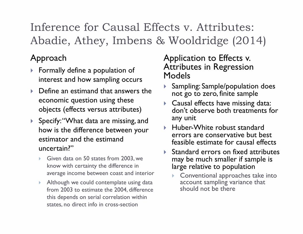
Inference for Causal Effects v. Attributes:Abadie, Athey, Imbens & Wooldridge (2014)Approach Formally define a population of
interest and how sampling occurs
Define an estimand that answers the economic question using these objects (effects versus attributes)
Specify: “What data are missing, and how is the difference between your estimator and the estimanduncertain?” Given data on 50 states from 2003, we
know with certainty the difference in average income between coast and interior
Although we could contemplate using data from 2003 to estimate the 2004, difference this depends on serial correlation within states, no direct info in cross-section
Application to Effects v. Attributes in Regression Models Sampling: Sample/population does
not go to zero, finite sample Causal effects have missing data:
don’t observe both treatments for any unit
Huber-White robust standard errors are conservative but best feasible estimate for causal effects
Standard errors on fixed attributes may be much smaller if sample is large relative to population Conventional approaches take into
account sampling variance that should not be there

Robustness
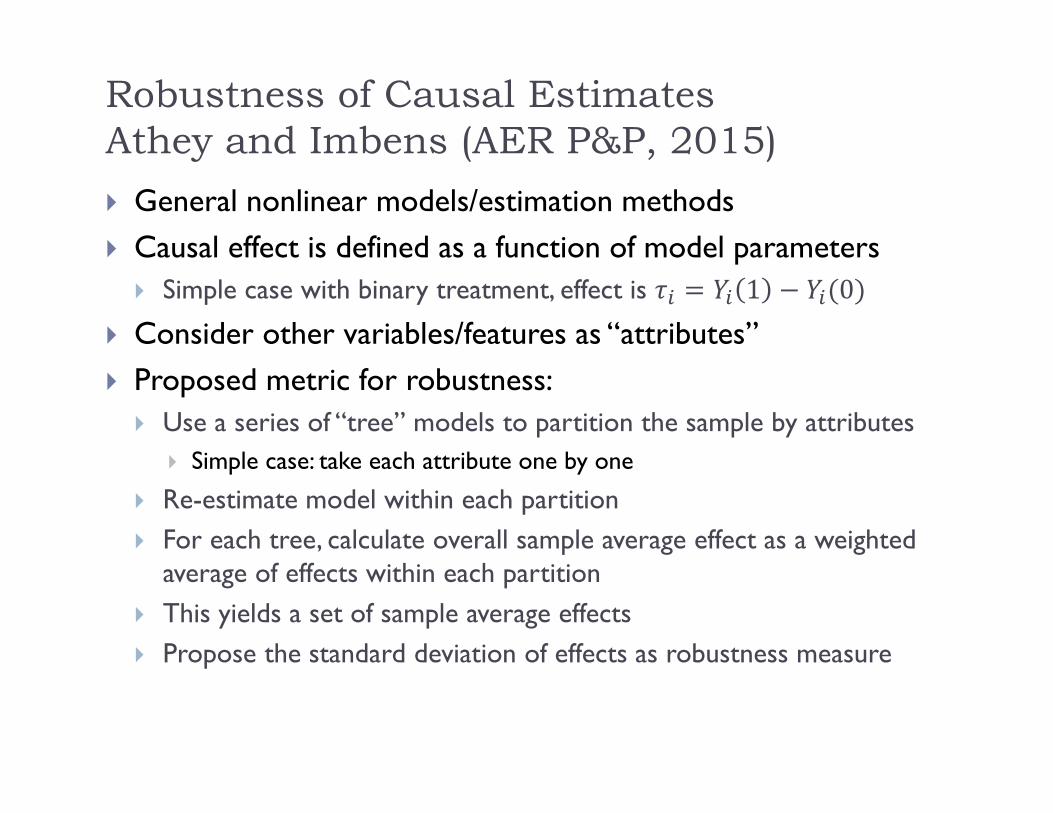
Robustness of Causal EstimatesAthey and Imbens (AER P&P, 2015) General nonlinear models/estimation methods Causal effect is defined as a function of model parameters Simple case with binary treatment, effect is 1 0
Consider other variables/features as “attributes” Proposed metric for robustness: Use a series of “tree” models to partition the sample by attributes
Simple case: take each attribute one by one
Re-estimate model within each partition For each tree, calculate overall sample average effect as a weighted
average of effects within each partition This yields a set of sample average effects Propose the standard deviation of effects as robustness measure
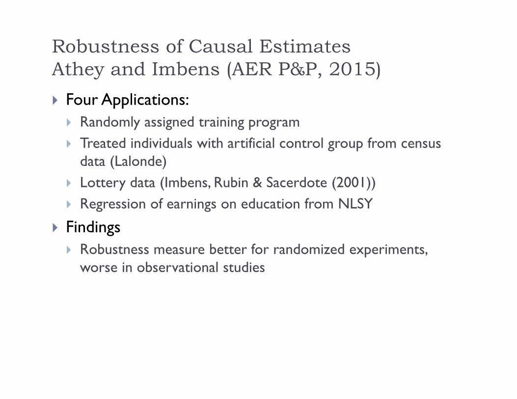
Robustness of Causal EstimatesAthey and Imbens (AER P&P, 2015) Four Applications: Randomly assigned training program Treated individuals with artificial control group from census
data (Lalonde) Lottery data (Imbens, Rubin & Sacerdote (2001)) Regression of earnings on education from NLSY
Findings Robustness measure better for randomized experiments,
worse in observational studies
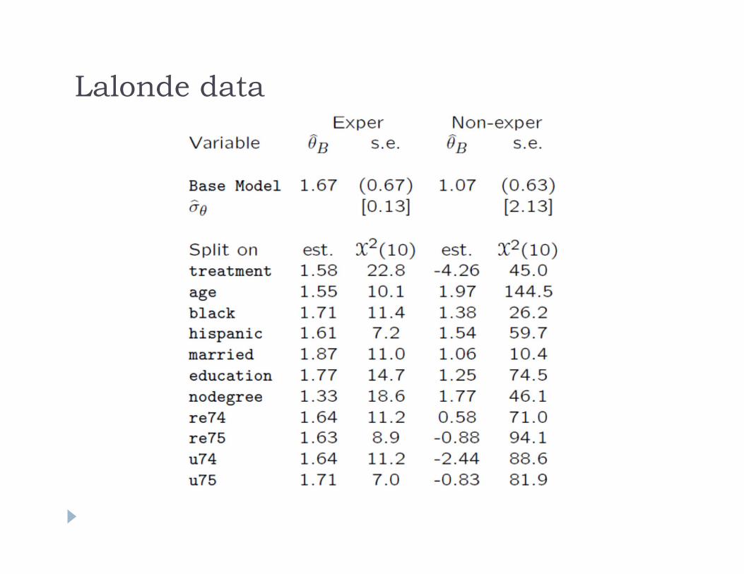
Lalonde data
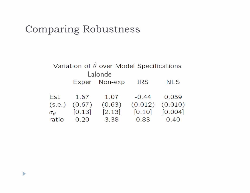
Comparing Robustness
Lalonde
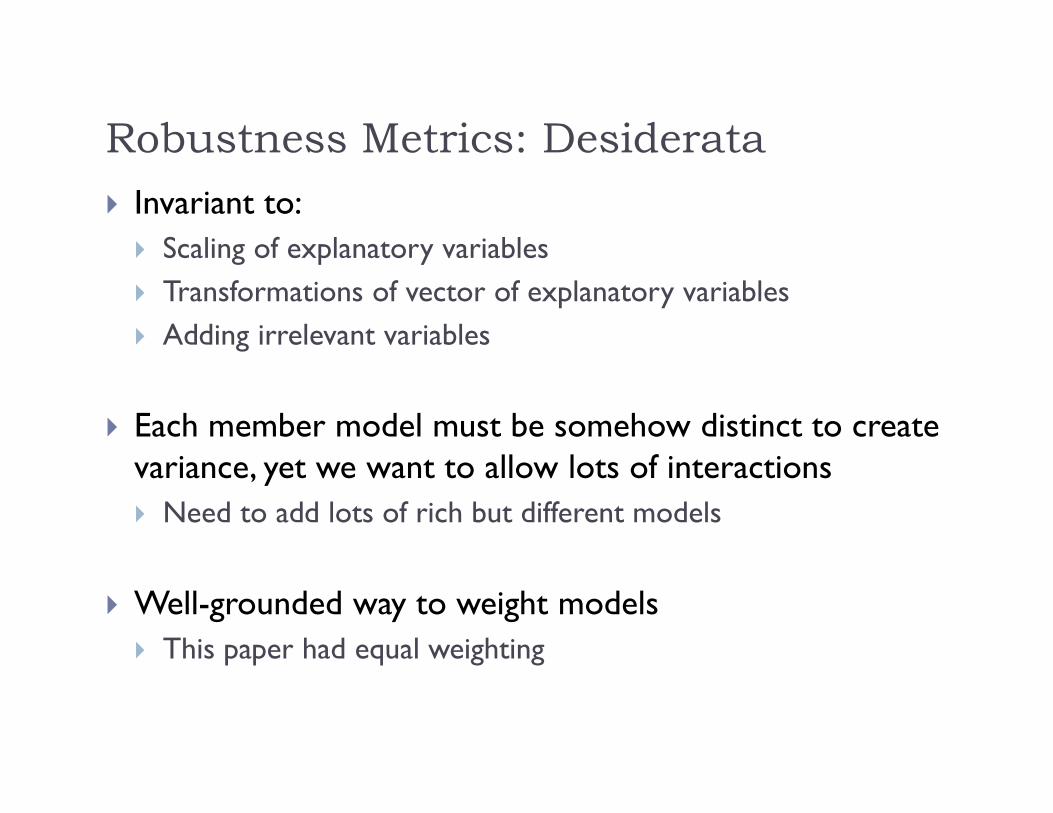
Robustness Metrics: Desiderata Invariant to: Scaling of explanatory variables Transformations of vector of explanatory variables Adding irrelevant variables
Each member model must be somehow distinct to create variance, yet we want to allow lots of interactions Need to add lots of rich but different models
Well-grounded way to weight models This paper had equal weighting
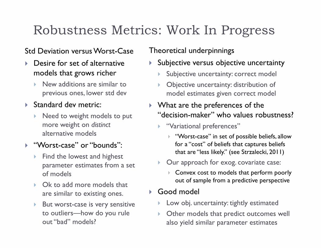
Robustness Metrics: Work In ProgressStd Deviation versus Worst-Case
Desire for set of alternative models that grows richer New additions are similar to
previous ones, lower std dev
Standard dev metric: Need to weight models to put
more weight on distinctalternative models
“Worst-case” or “bounds”: Find the lowest and highest
parameter estimates from a set of models
Ok to add more models that are similar to existing ones.
But worst-case is very sensitive to outliers—how do you rule out “bad” models?
Theoretical underpinnings
Subjective versus objective uncertainty Subjective uncertainty: correct model Objective uncertainty: distribution of
model estimates given correct model
What are the preferences of the “decision-maker” who values robustness? “Variational preferences”
“Worst-case” in set of possible beliefs, allow for a “cost” of beliefs that captures beliefs that are “less likely.” (see Strzalecki, 2011)
Our approach for exog. covariate case: Convex cost to models that perform poorly
out of sample from a predictive perspective
Good model Low obj. uncertainty: tightly estimated Other models that predict outcomes well
also yield similar parameter estimates
Conclusions on Robustness
ML inspires us to be both systematic and pragmatic
Big data gives us more choices in model selection and ability to evaluate alternatives
Maybe we can finally make progress on robustness


![Norma Nbe Ea-95[1]](https://img.pdfslide.net/doc/110x75/5572102e497959fc0b8cc019/norma-nbe-ea-951.jpg)