The Boom and the Depression: An Analysis within the Aggregate-Demand - Aggregate-Supply Framework

THE BOOM AND THE DEPRESSION:

AN ANALYSIS WITHIN THE

AGGREGATE-DEMAND –

AGGREGATE-SUPPLY FRAMEWORK

PEKKA SAURAMO*

LABOUR INSTITUTE FOR ECONOMIC RESEARCH

* This paper was finished during may stay at New York University as avisiting scholar. I would like to thank Jordi Gali for helpful comments.Responsibility for any remaining errors is my own. Financial support fromthe Yrjö Jahnsson Foundation is gratefully acknowledged.

LABOUR INSTITUTE FOR ECONOMIC RESEARCHDISCUSSION PAPERS 143

HELSINKI 1998

ISBN 952–5071–19–7ISSN 1236–7184

1 The interpretation could also be called the monetary explanation of thedepression. In the Finnish context this kind of characterization has a meaningdiffering from that common in the US discussion about the causes of the Great

3

1. INTRODUCTION

In Sauramo (1996) I started to analyse a most important and interestingperiod of Finnish economic history, the boom of the late eighties and thedepression of the early nineties, by utilizing an econometric model. Themain motivation for writing that paper was that the Finnish discussion aboutthe causes of the depression would benefit from research based on econo-metric analysis.

One of the aims of the paper was to assess the relative merits of thevarious explanations about the causes of the depression. In the paper Ioutlined the Finnish debate by distinguishing three interpretations of thedepression.

According to the first interpretation, the depression was mainly caused byfactors affecting exports, i.e. by the collapse of the Soviet trade, the deteri-oration of competitiveness and the worsening of international economicdevelopments. This explanation was called the interpretation based onthe traditional view of the Finnish business cycles as governed byfluctuations in exports.

By the second interpretation, the debt-deflation interpretation of thedepression, the ultimate cause of the depression was the false way ofliberalizing the financial markets during the eighties. The deregulationprocess led to a debt-driven boom and finally to a depression which wascharacterized by a Fisherian debt-deflation (Fisher 1932, 1933). Accordingto this interpretation, the depression was basically a monetary crisis duringwhich the credit channel played a major role.1

Depression. In the US debate, the monetary explanation of the Great Depressionhas traditionally been associated with monetarist explanations of the GreatDepression. For the US debate, see, for example, Brunner (1981). For the mostrecent Finnish studies, see Ahtiala (1997) and Kukkonen (1997). For earlier ones,see, for example, Sauramo (1991) and Söderström (1993).

4

The third interpretation was called the balance-of-payments interpreta-tion of the depression, since in the explanation the balance of paymentsconstraint is the most important part of the propagation mechanism throughwhich external shocks operate. According to this interpretation, the collapseof Soviet trade, the worsening of the terms of trade, the recession in theforeign economy and the rise in the foreign interest rates were able tocause the recession, because the balance of payments constraint magnifiedtheir negative effects (see Tarkka 1994). The biggest difference betweenthe first and third interpretation is that the most important propagationmechanism through which negative external shocks operate is assumed tobe different. Domestic demand has a more important role in the third thanin the first interpretation.

Hardly any discussant has supported only one of these interpretations, foreach of them only provides one view of the depression. Therefore, the”best” explanation of the depression is given by a synthesis of the threeinterpretations. This does not mean, however, that it is worthless to askwhich of the three views is the best one.

The approach used in Sauramo (1996) was similar to that of Blanchard(1993). Blanchard analysed the causes of the most recent recession in theUS by using a very simple two-variable structural VAR model. According toBlanchard’s analysis the main “cause” of the recession was a “consumptionshock”, an abnormal decrease in consumption. Analogously, the mainresult of Sauramo (1996), which utilized a four-variable (real GDP, privateconsumption, private investment, net exports) VAR model, was that con-sumption shocks played a major role both in the boom and the depression.Both the boom and the depression were consumption-led.

5

Therefore, one of the conclusions drawn in Sauramo (1996) was thatsomething essential is missing in the first interpretation, in which the role ofexports is highlighted. Negative shocks to net exports had a major influencein 1991 when GDP decreased by seven per cent, but they were not impor-tant at the onset of the depression which took place earlier. It was in 1991that the negative effects of the collapse of the Soviet trade were mostapparent.

A shock interpretation which is based on the dominant role of “consumptionshocks” is consistent with both the second and the third interpretation. Byusing only the results of Sauramo (1996), it is difficult persuasively to arguefor either of these two alternatives.

The interpretation of the “consumption shocks” was difficult, since theanalysis was, like that of Blanchard (1993), measurement without any wellarticulated theory. For example, they could be regarded as sudden realiza-tions of over-borrowing, an interpretation consistent with the second inter-pretation. But they could also reflect changes in expectations of futureincome, the changes being caused by worsening of the terms of trade.

The main aim of this paper is to deepen Sauramo’s (1996) discussion bylinking the econometric analysis more closely to economic theory. This isdone by estimating structural VAR models which are based on the utiliza-tion of the traditional aggregate-demand – aggregate-supply framework.Typically, these models belong to the class of IS-LM models, which havebeen augmented with a Phillips curve. Today this is one of the mostcommonly used frameworks in the empirical analysis of economic fluctua-tions.

Even though one can expect that the use of the aggregate-demand –aggregate-supply framework makes the interpretation of shocks easier thanthe use of a theoretical framework such as the one utilized in Blanchard(1993) or in Sauramo (1996), this does not mean that the interpretationbecomes easy.

2 For a discussion about the role of credit within the IS-LM framework, seeBernanke and Blinder (1988), and Brunner and Meltzer (1988).

3 For earlier attempts, see, for example, Cecchetti and Karras (1994), and Betts,Bordo and Redish (1996).

6

First, the framework should fit the data. In the case of Finland this is farfrom being obvious. Until the mid eighties, the financial markets wereregulated and therefore the standard textbook versions were more or lessinapplicable in the description of the behaviour of the economy. Since thederegulation of the financial markets the situation has changed, but shiftsin the exchange rate policy and monetary policy regimes complicate theuse of the standard IS-LM framework or its cousin, the Mundell-Flemingframework.

Second, the shock interpretation should be useful when one discusses therelative merits of the various explanations of the causes of the depression.Obviously, it is difficult to construct a variant of the aggregate-demand –aggregate-supply model by which one could assess all the relevant aspectsof the depression. At least, the model should enable one to comment onthe most important standpoints of the debate. This means, first of all, thatone could analyse the role of credit and the credit channel. Since credithas no role within the standard textbook versions of the aggregate-demand– aggregate-supply model, or within the IS-LM model, it is not clear how thevalidity of the second interpretation can be assessed by these models.2

It will be seen that it is not impossible.3 Yet it will also be seen that it is noteasy to find a theoretical framework on which the Finnish debate about thecauses of the depression should be based. Therefore, the analysis of thispaper will still be tentative.

The results of this paper mainly serve the assessment of the relative meritsof the second and the third interpretation. Because the role of the terms oftrade is central in the third interpretation, the importance of changes in theterms of trade during the past ten years deserves special attention.

7

This paper is organized as follows. In the next chapter, the framework ofthe investigation is introduced. Chapter 3 discusses the data. Chapter 4contains the main results, and Chapter 5 concludes the work.

4 The major alternative has been to build the analysis upon Real Business Cycletheory.

5 Models which are augmented with a Phillips curve can be illustrated by ananalogous figure in inflation – output space.

8

2. THE FRAMEWORK

The aggregate-demand – aggregate-supply framework

A large number of recent econometric studies which utilize structural VARmodels in the description of economic fluctuations have the traditionalaggregate-demand – aggregate-supply framework as the point ofdeparture.4 Within that framework, the shocks that are the main sources offluctuations are either aggregate-demand or aggregate-supply shocks.Figure 1, of which there are numerous examples in various textbooks,illustrates how one can distinguish between these two types of shocks (see,for instance, Bergman 1992, Chapter 4, and Sterne and Bayoumi 1993).5

9

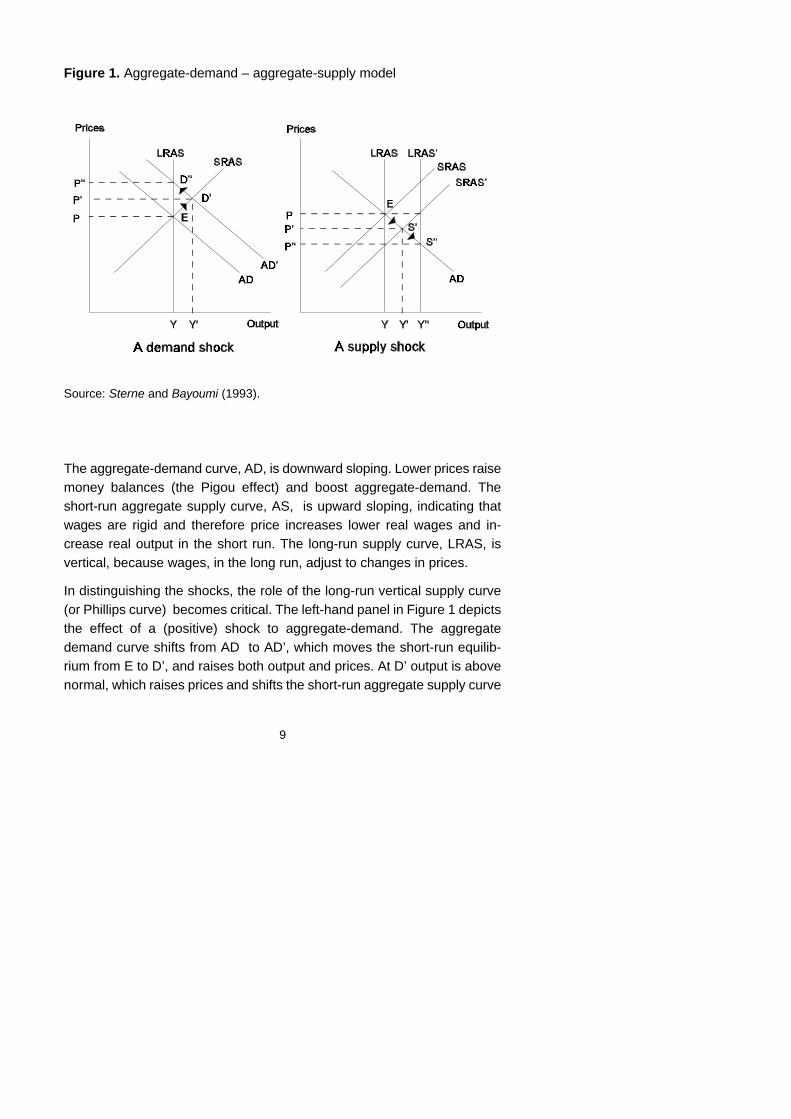
Figure 1. Aggregate-demand – aggregate-supply model

Source: Sterne and Bayoumi (1993).

The aggregate-demand curve, AD, is downward sloping. Lower prices raisemoney balances (the Pigou effect) and boost aggregate-demand. Theshort-run aggregate supply curve, AS, is upward sloping, indicating thatwages are rigid and therefore price increases lower real wages and in-crease real output in the short run. The long-run supply curve, LRAS, isvertical, because wages, in the long run, adjust to changes in prices.

In distinguishing the shocks, the role of the long-run vertical supply curve(or Phillips curve) becomes critical. The left-hand panel in Figure 1 depictsthe effect of a (positive) shock to aggregate-demand. The aggregatedemand curve shifts from AD to AD’, which moves the short-run equilib-rium from E to D’, and raises both output and prices. At D’ output is abovenormal, which raises prices and shifts the short-run aggregate supply curve

10

upwards. The economy moves gradually to the new long-run equilibrium D’’where the price level is higher than at E but output is at its initial level.Thus, a positive demand shock is expansionary and inflationary in the shortrun, but in the long run it only raises the price level.

The effect of a positive supply shock is depicted in the right-hand panel ofthe figure. The shock (for instance, a favourable technology shock or anincrease in labour supply) shifts the short- and long-run supply curvesrightwards. This raises output and reduces prices, moving the short-runequilibrium from E to S’ first. At S’ output is below the new long-run level,which decreases prices and shifts the short-run supply curve downwards.Output increases and prices decrease until the new equilibrium S’’ isachieved. The important difference between aggregate-demand andaggregate-supply shocks is that positive aggregate-supply shocks havepermanent positive effects on real output. Furthermore, positive supplyshocks are deflationary. They reduce prices.

The classification of shocks into aggregate-demand and aggregate-supplyshocks rests on the assumption about the vertical long-run supply (orPhillips) curve. If that is assumed to exist, aggregate-demand shocks donot affect output in the long-run. Obviously, this assumption is problematic,because it is easy to think of channels through which demand shocks mayhave long-lasting, or even permanent, effects on output (capitalaccumulation, hysteresis in the labour market, increasing returns to scaleetc.) Blanchard and Quah (1989), who were among the first to apply theaggregate-demand – aggregate-supply framework in the identification ofthe shocks, noted – and proved – that if the (permanent) effects ofaggregate-demand shocks are small relative to those of aggregate-supplyshocks, the identification of the shocks can be based on the assumptionthat aggregate-demand shocks have no long-run effects on output.

I will report results from various experiments which are based on the use ofthe aggregate-demand – aggregate-supply framework. Also, I will discussits validity in the Finnish context.

11

)yt

)pt

'A(L),st

,dt

, (1)

B(L)xt'<t, (2)

Identification of shocks

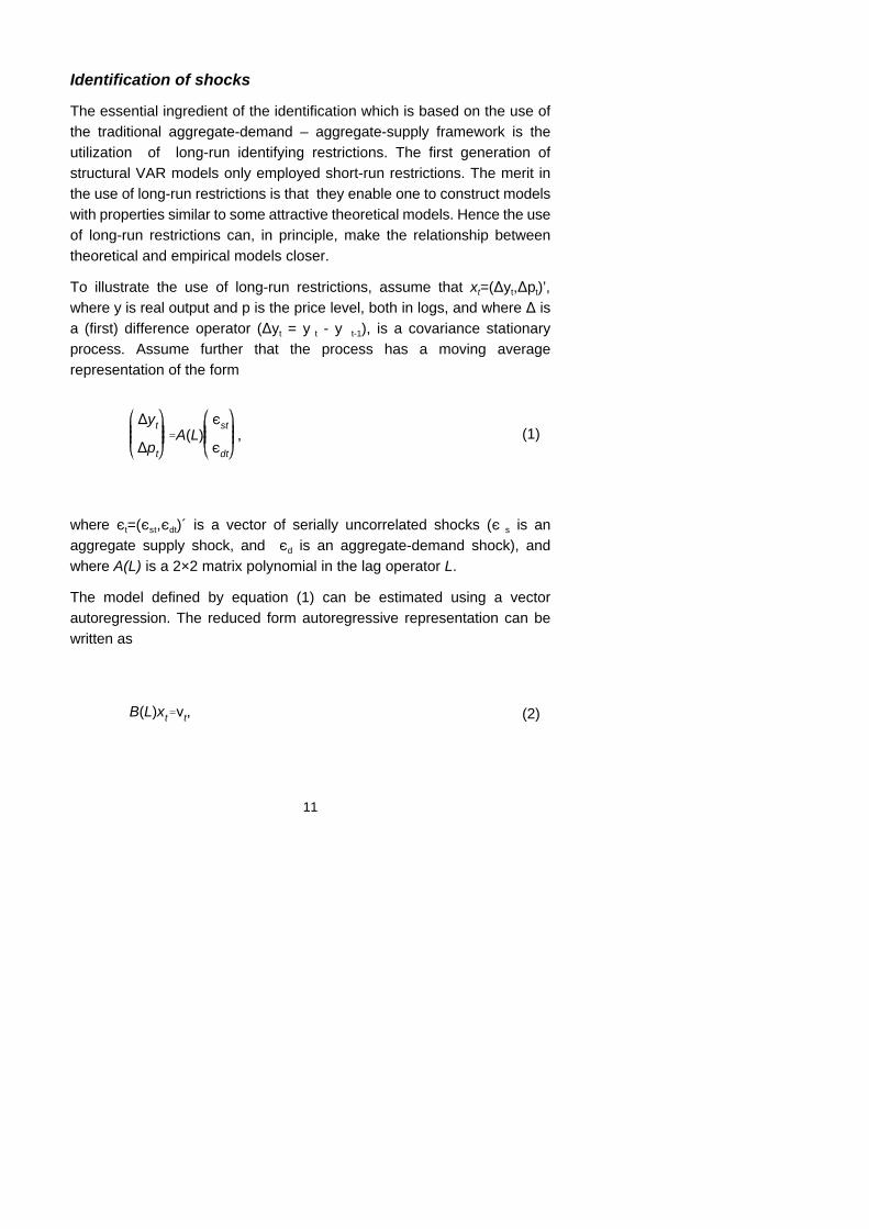
The essential ingredient of the identification which is based on the use ofthe traditional aggregate-demand – aggregate-supply framework is theutilization of long-run identifying restrictions. The first generation ofstructural VAR models only employed short-run restrictions. The merit inthe use of long-run restrictions is that they enable one to construct modelswith properties similar to some attractive theoretical models. Hence the useof long-run restrictions can, in principle, make the relationship betweentheoretical and empirical models closer.

To illustrate the use of long-run restrictions, assume that xt=()yt,)pt)’,where y is real output and p is the price level, both in logs, and where ) isa (first) difference operator ()yt = y t - y t-1), is a covariance stationaryprocess. Assume further that the process has a moving averagerepresentation of the form

where ,t=(,st,,dt)´ is a vector of serially uncorrelated shocks (, s is anaggregate supply shock, and ,d is an aggregate-demand shock), andwhere A(L) is a 2×2 matrix polynomial in the lag operator L.

The model defined by equation (1) can be estimated using a vectorautoregression. The reduced form autoregressive representation can bewritten as

12

<t'S,t, (3)

A(L)'B(L)&1S. (4)

SS )'E, (5)

where < is the vector of residuals, B(L)/[Bij] for i,j=1,2, and B(0)=I.

The residuals are assumed to be linear combinations of the shocks, i.e. thestructural disturbances. Therefore

where S is non-singular. Equations (1) and (2) imply that

Matrix A(L) can be estimated by using the estimated coefficients of B(L)and by using some identifying restrictions by which the four elements ofmatrix S can be determined.

In the 2×2 case, four constraints are needed for just-identification. Threeconstraints are given by the assumption that the shocks are mutuallyorthogonal and that their variances equal to unity.

These constraints imply that

where G=E<<’ (E denotes the expectational operator). Equation (5)provides three quadratic equations.

The fourth restriction is given by the assumption that in the long run theaggregate-demand shocks do not affect output .

The long-run effects of the shocks are given by the elements of A(1):

13

A(1) '

ays ayd

aps apd

(6)

The restriction that the aggregate-demand shocks have no long-run effectson output implies that ayd =0. The fourth equation can be defined by using(4), which implies that A(1)=B(1)-1 S.

In the 2×2 case, one additional constraint, in addition to orthogonalityconditions, is enough for just-identification. In more general cases, moreconstraints (in addition to orthogonality conditions) are needed. In theirpioneering work, Blanchard and Quah (1989) estimated a bivariatestructural VAR model by using one long-run constraint.

Bivariate models have the disadvantage that one cannot identify separatecomponents of the aggregate demand and supply shocks. Gali (1992)estimated, by utilizing both short-run and long-run restrictions, a four-variable model by which he was able to identify four types of shocks:aggregate- supply shocks, money-supply shocks, money-demand shocks,and IS shocks. Hence, he identified three separate aggregate-demandshocks and estimated an IS-LM model which is augmented with the Phillipscurve. In some studies, aggregate-supply shocks have also been separatedinto components. For example, Shapiro and Watson (1988) estimated afour-variable model by which they separated aggregate-supply shocks intotwo components: labour-supply and technology shocks.

As pointed out in the introduction, the identification of shocks within theaggregate-demand – aggregate-supply framework is not straightforward inthe case of Finland. Therefore, I have estimated various models all ofwhich belong to the class of aggregate-demand – aggregate-supply models.I will report and discuss results which are based on the estimation of two-,three-, four-, and five-dimensional structural VAR models.

14

3. THE DATA

I utilize data on variables, which enables the discussion about the causes ofthe depression, which can be included in a model which belongs to theclass of traditional aggregate-demand – aggregate-supply models, andwhich fits the data as well as possible. Yet, because the dimension of VARmodels cannot be very high, it is impossible to include all the potentiallyrelevant variables in the model.

The choice of variables is critical, since it largely determines the nature ofconceivable shock interpretations. In Sauramo (1996), the exploration wasbased on the examination of the joint behaviour of four variables: realGDP, private consumption, private fixed investment and net exports. Eventhough one can achieve reasonable and interesting results also by utilizingthis kind of set of variables, the analysis is bound to be measurementwithout any well-articulated economic theory. The variables used in thisstudy (should) tie the investigation about the causes of the boom anddepression more closely to economic theory.

The following variables are utilized in the analysis: real GDP (denoted byY), real private consumption (C), consumer prices (P), short-term interestrate (r), and the terms of trade (TOT). (Except for r, lower case letters areused to denote the logs of the variables.)

The choice of Y and P is obvious, if one wants to identify aggregate-demand and aggregate-supply shocks (see Figure 1). The use of rmakes the examination of the role of real interest rate movements, and ofmonetary policy, possible. Also, it may be useful if one attempts toseparate, in the spirit of the IS-LM model, aggregate-demand shocks intoIS- and LM-shocks (see, for instance, Gali 1992). The choice of privateconsumption is not obvious, if one is searching for “ultimate” causes of the

6 For a discussion of “consumption shocks”, see also Cochrane (1994).

7 For the use of such models, see, for instance, Erkel-Rousse and Melitz (1995)and Schön (1995).

15

boom and the depression. Essentially, private consumption is anendogenous variable, which makes the interpretation of “consumptionshocks” very difficult. This was demonstrated by Blanchard (1993) andSauramo (1996).6 There are two closely related reasons for choosingprivate consumption as one of the variables.

According to the previous study, “consumption shocks” played a major roleboth in the boom and the depression. Both the boom and the depressionwere consumption-led. This strongly motivates the use of consumption asone explanatory variable even if the interpretation of these shocks wasvery difficult. But one can make progress in interpreting these shocks ifprivate consumption is one variable in a model which is more closely tiedwith economic theory. Furthermore, in the second interpretation of thecauses of the depression the role of credit and the credit channel isunderlined. The inclusion of private consumption can make the examination(or, the speculation) of the role of credit (and the debt-deflation process)easier, even though the standard aggregate-demand – aggregate-supplymodels, or IS-LM models, allow no explicit role for credit (see, forexample, Bernanke and Blinder 1988).

The terms of trade have been chosen as one of the variables because, bythe third interpretation about the causes of the depression, it has played animportant role in shaping the nature of economic developments during thepast ten years.

One can argue that some very relevant variables will be missing in themodels. Since Finland is a small open economy, one could expect thatvariables such as net exports and the real exchange rate would enter themodels, and a theoretical model which belongs to the class of Mundell-Fleming models would serve as a baseline model.7

16

The choice of variables is based on experimenting, also with variables likethe real exchange rate. One conclusion which could be drawn from theseexperiments is that factors which operate through the real interest rateseem to have been more important that those operating through the realexchange rate. This has been one reason for omitting the real exchangerate. Furthermore, if one wants to undertake a careful analysis about thevalidity of the second interpretation about the depression, the real interestrate is a natural choice. In principle, both variables could, and should, enterthe relevant models. According to my experiments, which have still beententative, that would have complicated the analysis substantially withoutany noticeable payoff.

As noted earlier, the exploration will be based on the estimation of two-,three-, four-, and five-variable models. This means that not every variableenters every model.

The estimations will be based on quarterly data which cover the period1975:1–1996:2. Quarterly data on GDP, private consumption and theterms of trade are from the quarterly national accounts constructed byStatistics Finland. Deflators for exports of goods and services, and importsof goods and services were used when the series for the terms of trade wasconstructed. Consumer prices are measured by the Consumer PriceIndex. Series for short-term interest rates are difficult to construct for thewhole period under consideration, because owing to the regulation of thefinancial markets there does not exist an unbroken series for short-terminterest rates. The interest rate series was constructed by splicing togethertwo series. For the period from the first quarter of 1975 to the fourthquarter of 1986, the data have been constructed by utilizing data on three-month eurodollar rates and the discount of the FIM relative to the US dollaron three-month futures trades. From the first quarter of 1987 the data is onthree-month Helibor rates.

Except for data on interest rates, the series are seasonally adjusted.

According to the standard augmented Dickey-Fuller tests, y, c, r, and tothave a unit root and are therefore I(1) variables. The best way to

17

characterize p is to regard it as a I(2) variable. Most of the analyses areperformed under this assumption.

In the remainder of the paper, I report results from the exercises I made byutilizing the above data and by estimating two-, three-, four- and five-dimensional structural VAR models. Cointegration properties of the data arediscussed when these models are specified and estimated.

18

4. RESULTS

The benchmark case: a bivariate VAR model

The identifying restriction used by Blanchard and Quah (1989) is attractive,because it is powerful. It enables one to separate aggregate-demand andaggregate-supply shocks by utilizing a very simple bivariate VAR model.Blanchard and Quah employed a model which desribes the joint behaviourof GNP and unemployment rate. This choice is only one alternative. Forinstance, in Bayoumi and Eichengreen (1994), Bergman (1992), Gerlachand Klock (1991), and Sterne and Bayoumi (1993) data on GDP and priceswere used in the identification. This is what is done in this paper, too.

I estimate a bivariate model using data on GDP and consumer prices, andemploying the restriction that aggregate-demand shocks do not affectoutput in the long run. According to the aggregate-demand – aggregate-supply model, positive demand shocks should raise consumer prices bothin the short and in the long run, while positive supply shocks should reduceprices. These responses are not imposed, however. Therefore they canserve as over-identifying restrictions when the sensibility of the results isdiscussed.

My ultimate aim is to describe and analyse the boom and the depression byestimating a four- or five-variable model by which one could separate fouror five shocks. The basic reason for starting the exploration by using abivariate model is that, as will be seen, it is not at all easy to identify, byusing the Finnish data, shocks which have interpretations consistent withthe traditional aggregate-demand – aggregate-supply model. This can bedemonstrated by a bivariate model.

I report results which were based on the assumption that y and p are I(1)variables, which means that xt = ()yt, )pt)’ is assumed to be a covariance

8 Consequently, the model was estimated in the difference form. Three lags wereused, with Schwarz and Hannan-Quin information criteria being the main decision-making criteria. The estimation period was 1976:1–1996:2.

9 I also did the same exercises by using the GDP deflator instead of theConsumer Price Index. The results remained essentially the same.

19

stationary process.8 The results would remain qualitatively the same if p isassumed to be an I(2) variable.9

The characteristics of the shocks will be illustrated by using impulseresponses and forecast error variance decompositions. The importance ofthe various shocks in shaping the boom and depression years are illustratedby using historical forecast error decompositions.

Figures 2 and 3 display the responses of GDP and consumer prices to apositive permanent and transitory shock, respectively. The permanentshock has a permanent positive effect on output. If it is to be called asupply shock, it should decrease prices. Yet this is not the case. The shockis inflationary. Also, the interpretation of the transitory shock is difficult.Like a positive aggregate-demand shock, it is inflationary, but it reducesoutput. It looks like a temporary negative supply shock. (Within an openeconomy framework the shock still can be regarded as an aggregate-demand shock: inflationary aggregate demand shocks may becontractionary, if they lead to a deterioration of competitiveness.)

Figure 2. Dynamic responses to a permanent shock: a bivariate model

0 10 20 30 40GDP

0.00

0.01

0.02

0.03

LOG

0 10 20 30 40PRICE LEVEL

0.00

0.01

0.02

0.03

0.04

LOG

20

Figure 3. Dynamic responses to a transitory shock: a bivariate model

0 10 20 30 40GDP

-0.01

0.00

0.01

LOG

0 10 20 30 40PRICE LEVEL

0.00

0.01

0.02

0.03

0.04

LOG

In principle, positive supply shocks can be associated with increasing pricesif, for instance, monetary policy authorities (over)react to such a shock byloosening the stance of monetary policy more than required. In that caseimpulse responses in Figures 2 and 3 would also reflect monetary policyreactions to positive supply shocks. At least in the case of Finland, thisexplanation is hardly plausible.

Finland is not the only country which may be associated with inflationarypermanent shocks. Bayoumi and Eichengreen (1994) found that thisproperty is common to those countries which are heavily dependent on rawmaterial production. They argue (on page 13) that this may reflect the factthat, for raw material producers (like Indonesia, Maleysia, and Norway),positive supply shocks are associated with improvements in the terms oftrade, which boost aggregate demand, and, consequently, increase prices.However, this explananation may not apply to Finland, because changes inthe terms of trade in Finland seem to be independent of other shocks. Thistopic will be discussed later.

The first exercise demonstrates that, that the Finnish data is used, theshocks which are obtained using the Blanchard-Quah identification may notbe consistent with the conventional aggregate-demand – aggregate-supplymodel.

10 When GDP deflator is used instead of the Consumer Price Index, theimportance of transitory shocks increases somewhat but it is still minor.

21

This is not the first time that one obtains inflationary permanent shocks byusing Finnish data and by using restrictions analogous to those used above.Mellander, Vredin and Warne (1990) obtained a similar result when theyexamined the joint dependence of six variables: GDP per capita,consumption (private and public) per capita, gross fixed investment percapita, terms of trade, GDP deflator, and nominal money stock per capita(M2). They utilized yearly observations from the period 1866–1985. It isworth noting that for Sweden the results were in line with the aggregate-demand – aggregate-supply framework. On the other hand, Sterne andBayoumi (1993) were able to identify sensible supply shocks for Finland byutilizing a bivariate VAR model similar to that used in this paper and byusing yearly observations from the period 1963–1988. Furthermore,Hartikainen (1995) could identify reasonable aggregate-demand andaggregate-supply shocks by utilizing, like Blanchard and Quah (1989),quarterly data on GDP and unemployment from the period 1970–1990, andfrom the subperiods 1970–1983, and 1984–1990.

Table 1 illustrates the relative importance of the two shocks. Fluctuations ofGDP are almost completely attributable to permanent shocks.10

The dominant role of the permanent shocks is also seen in Table 2, whichdisplays the decomposition of eight-quarter forecast errors for GDP.(Figures are yearly averages, which have been calculated by usingquarterly observations. Eight quarters were chosen, because the peaks andtroughs correspond closely enough to the peaks and the troughs of theGDP series.) Both the boom and the depression were caused by thepermanent shocks.

The figures in Table 2 should be interpreted as follows. In 1986 the eight-quarter forecast error for GDP was 0.7 per cent, i.e. the realized level ofGDP was 0.7 per cent higher than that forecast by the model. (Owing to the

22

Table 1. Forecast-error variance decompositions for GDP: output – pricesmodel

Horizon in quarters Permanent shock Transitory shock

Contemporaneous 4 8 12 16 20 24100

97.596.997.598.098.598.899.099.8

2.53.12.52.01.51.21.0 .2

Note: In the table the forecast error variances have been decomposed to twosources. For instance, of the 8-step forecast error variance of GDP, 97.5 per centis accounted for by permanent shocks and 2.5 percent by transitory shocks.

Table 2. Decomposition of eight-quarter forecast errors for GDP: output –prices model (yearly averages for 1986–1995)

Year GDP Permanent shock Transitory shock

1986198719881989199019911992199319941995

0.7 1.5 4.6 5.4 0.0 -13.4 -13.8 -4.8 1.3 0.6

-0.2 1.1 4.8 5.6 0.0-13.1-12.8 -4.2 0.9 0.5

0.9 0.4 -0.2 -0.2 0.0 -0.3 -1.0 -0.6 0.4 0.1

Note: Forecast errors of the first column are based on the use of the level form ofthe model. Consequently, the forecast errors have been obtained by subtracting theforecasts from the logs of the realized levels of GDP.

11 For a discussion, see, for example, Bernanke and Blinder (1992), Sims (1992)and Strongin (1995).

23

way the forecast errors are computed, see the note in Table 2; they are notexactly the same as relative forecast errors. The difference, however, issmall.) Of this error, -0.2 percentage points were due to the permanentshock, and 0.9 percentage points to the transitory shock, respectively.

According to Table 2, permanent shocks caused both the boom and thedepression with transitory shocks playing only a minor role. Yet this resultis hard to interpret, because it is very difficult to say what these permanentshocks are. According to the vertical Phillips curve paradigm they should bepermanent supply shocks, but the impulse response analysis did notconfirm this interpretation. Rather, they looked like permanent demandshocks.

Obviously, there is need for further investigation. The resuIts may be due toomitted variable bias, which is one reason for the use of larger models.

A three-variable model

A natural extension of the above model is a three-variable model whichallows for the separation of three shocks: one aggregate-supply shock andtwo aggregate-demand shocks. If one wants to identify shocks which maybe interpretable within the IS-LM framework, the three variables can be, forinstance, GDP, consumer prices and short-term interest rates. By usingthese variables, the aggegate-demand shocks can, in principle, beseparated into IS and LM shocks or to monetary policy shocks.

Cecchetti and Karras (1994), relying on Gali (1992), employed this kind ofmodel, and also other models, when they examined the causes of the GreatDepression in the US. Gerlach and Smets (1995) also utilized a similarmodel. The use of this kind of model can be motivated by the argumentthat it is rather a short-term interest rate than a monetary aggregate that isthe relevant policy instrument.11 This assumption enables one to analyse

12 Because the interest rate was measured as an annual percentage, inflation wasmeasured in an analogous manner: )p = 400ln(Pt /Pt-1 ).

24

the role of monetary policy without the use of a monetary aggregate. Gali(1992), however, used a four-variable model with a monetary aggregate(M1) as an additional variable, and was able to separate four types ofshocks: aggregate-supply shocks, IS shocks, money-demand shocks, andmoney-supply shocks.

In the case of Finland, the above motivation is not very persuasive,however. During the past twenty years Finland has experienced drasticchanges in the institutional environment within which monetary andexchange rate policies have been conducted. That period also embracesdifferent monetary and exchange rate policy regimes. Therefore, for mostof the time, changes in short-term interest rates may not have been due tothe decisions taken by the monetary authorities. Rather, they may havereflected changes in the expectations on the future value of the FIM.

Even though it will not be easy to interpret the shocks which have beentransmitted to the real sector through changes in real interest rates, thistransmission channel, has, however, been important in Finland , especiallyduring the past ten years. This motivates the subsequent analysis.

The estimation of the model is based on the assumption that ()yt ,)rt ,rt -)pt)’, where r -)p is the real interest rate, is a covariance stationaryprocess.12 As noted earlier, it is reasonable to assume that y and r are I(1)variables. Furthermore, it is sensible to assume that also )p is an I(1)variable. On the other hand, according to the standard Dickey-Fuller testsr-)p is an I(0) variable. Therefore r and )p are assumed to be cointegratedwith (1,-1)’ being the cointegration vector.

The resulting system describes the joint behaviour of GDP, nominal, andreal interest rates. By using the model it is also possible to analyse howinflation (or the price level) responds to the various shocks. This means thatresponses of inflation (or the price level) can serve as an over-identifyingrestriction by which the sensibility of the results can be assessed.

25

The identification of shocks is a straightforward generalization of theprocedure presented earlier. The just-identification of shocks requires theuse of nine restrictions. Six of them are provided by the orthogonality andnormalization conditions. The remaining three are given by the followingassumptions. Because the purpose is to identify two aggregate-demandshocks, it is asumed that neither of them has a permanent effect on realoutput. This gives two restrictions. The third assumption is the same which,for example, Gali (1992) used when he separated LM shocks from ISshocks. He assumed that, unlike IS shocks, neither money demand normoney supply shocks affect output contemporaneously. Within the three-variable framework it means that monetary (policy) disturbances areassumed not to affect output within the quarter. This assumption about thepresence of outside lag was also used by Cecchetti and Karras (1994), andGerlach and Smets (1995).

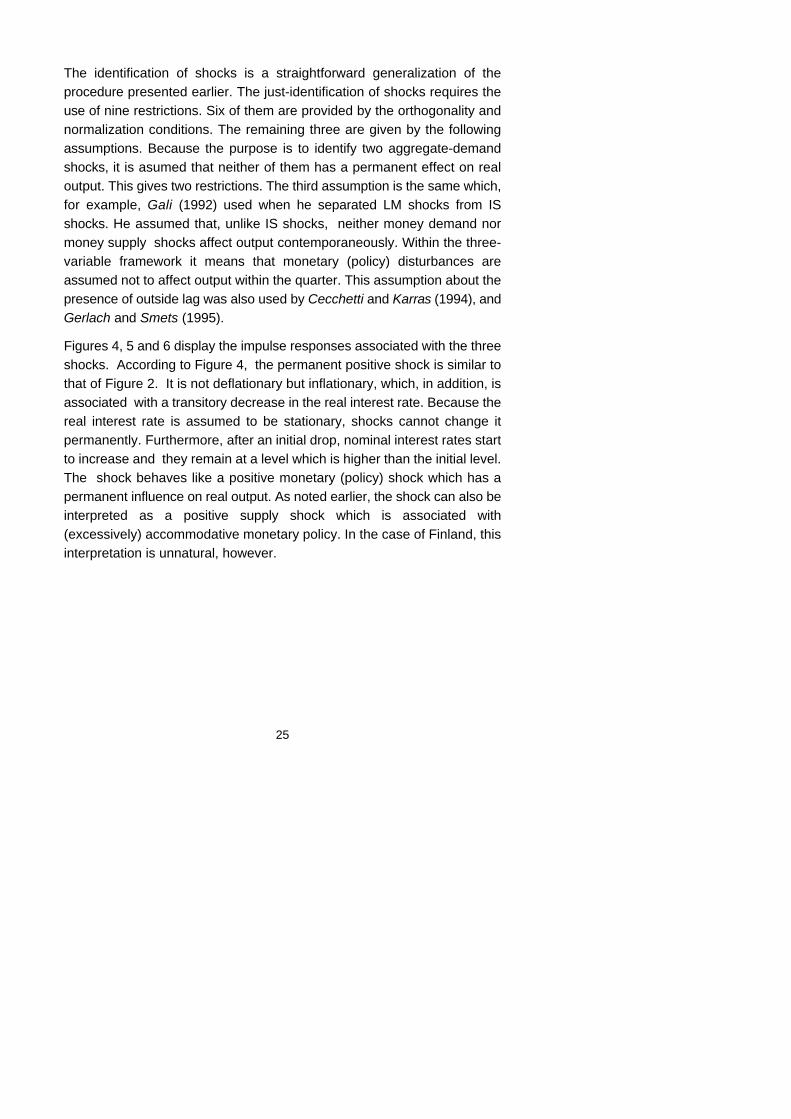
Figures 4, 5 and 6 display the impulse responses associated with the threeshocks. According to Figure 4, the permanent positive shock is similar tothat of Figure 2. It is not deflationary but inflationary, which, in addition, isassociated with a transitory decrease in the real interest rate. Because thereal interest rate is assumed to be stationary, shocks cannot change itpermanently. Furthermore, after an initial drop, nominal interest rates startto increase and they remain at a level which is higher than the initial level.The shock behaves like a positive monetary (policy) shock which has apermanent influence on real output. As noted earlier, the shock can also beinterpreted as a positive supply shock which is associated with(excessively) accommodative monetary policy. In the case of Finland, thisinterpretation is unnatural, however.

26

Figure 4. Dynamic responses to the permanent shock: output – nominalinterest rate – real interest rate model

0 10 20 30 40GDP

0.00

0.01

0.02

0.03

LOG

0 10 20 30 40NOMINAL RATE

-0.8

-0.4

0.0

0.4

0.8

PE

RC

EN

T

0 10 20 30 40REAL RATE

-1.4

-1.0

-0.6

-0.2

0.2

PE

RC

EN

T

0 10 20 30 40INFLATION

0.00

0.30

0.60

0.90

PE

RC

EN

T

The most salient feature of the transitory shock, which was based on theassumption about outside lag, is that a rising interest rate is associatedwith increasing prices (Figure 5). It can be regarded as an inflation shock,which is associated with a rise in the nominal interest rate and a fall in thereal interest rate. It has a slight negative effect on real output. That maynot be significant statistically, however. (As noted earlier, within an openeconomy framework, inflationary shocks, even though they cause a fall inthe real interest rate, may be contractionary if they lead to a deterioration ofcompetitiveness.) This shock, which is similar to the transitory shock in thecase of the bivariate model, can hardly be interpreted as a (monetary)policy shock.

27

Figure 5. Dynamic responses to the 1st transitory shock: output – nominalinterest rate – real interest rate model

0 10 20 30 40GDP

-0.01

0.00

0.01

LOG


0.0

0.2

0.4

0.6

0.8

1.0

PE

RC

EN

T

0 10 20 30 40REAL RATE

-1.2

-1.0

-0.8

-0.6

-0.4

-0.2

0.0

0.2

PE

RC

EN

T


0.00

0.50

1.00

1.50

2.00

PE

RC

EN

T

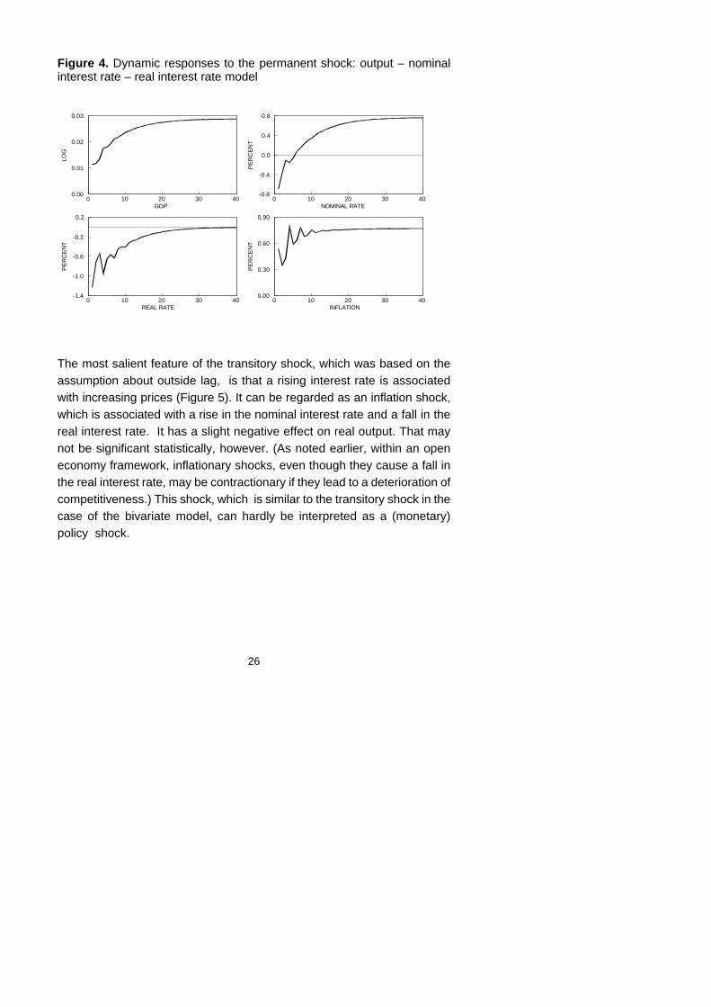
The other transitory shock is difficult to interpret (Figure 6). Consistent witha response to a positive aggregate-demand shock, it is associated with arise both in the real and nominal interest rate. Yet the shock is deflationary.

13 Adding one variable did not bring about essential changes either in forecasterror variance decompositions or in historical forecast error decompositions. Therole of permanent shocks remained dominant. These tables are available uponrequest.

28

Figure 6. Dynamic responses to the 2nd transitory shock: output – nominalinterest rate – real interest rate model

0 10 20 30 40GDP

-0.01

0.00

0.01

LOG


-0.6

0.0

0.6

1.2

1.8

PE

RC

EN

T

0 10 20 30 40REAL RATE

-0.5

0.0

0.5

1.0

1.5

2.0

2.5

PE

RC

EN

T


-0.6

-0.3

0.0

0.3

PE

RC

EN

T

All in all, adding one variable (a nominal interest rate) did not provide asolution to the problem which was already demonstrated by the bivariatemodel.13 The shocks are very difficult to interpret within the traditionalaggregate-demand – aggregate-supply framework which is based on theassumption about the vertical long-run Phillips curve. According to theimpulse response functions, the permanent shock seems to be anaggregate-demand and not an aggregate-supply shock. The results are incontrast with those obtained, for instance, by Gerlach and Smets (1995) forthe G-7 countries. The authors were able to get evidence which wasconsistent with the framework.

29

The results obtained so far have been so puzzling that they motivate furtherinvestigation. It is possible that, like the bivariate model, the three-variablemodel, too, suffers from omitted variable bias, which led to themisspecification of the model. The most unappealing feature of the resultswhich have been reported so far is that permanent shocks behave likeaggregate-demand shocks and not like aggregate-supply shocks. One cantry to improve the model by using variables which, by controlling for factorsaffecting aggregate-demand, make a further separation of aggregate-demand shocks possible.

A four-variable model: one permanent shock

One natural candidate for the fourth variable is a monetary aggregate.Adding a monetary aggregate would enable one to conduct an investigationsimilar to that of Gali (1992). On the other hand, Gerlach and Smets (1995)report (note 5 on page 8) that in preliminary work they included monetaryaggregates in the analysis but found that they were largely determined bymoney-demand shocks which have little impact on the economy. Theyinterpret these findings to reflect that monetary aggregates are dominatedby disturbances which are unrelated to the state of monetary policy, forinstance, by financial deregulation. This leads to difficulties in theidenfication of monetary policy shocks. According to my experiments, thisis the finding which applies to Finland, too. Adding a monetary aggregatewill not solve the identification problem, for the reasons Gerlach and Smets(1995) presented. After the above experiments with the three-variablemodel, this is not surprising.

Therefore, it seems to be very difficult to find exogenous (policy) variableswhich would be useful in explaining the boom and the depression.Consequently, one has to rely on the use of endogenous variables, whichmay allow for a reasonable interpretation. For reasons already presentedearlier (on page 10), and for controlling factors affecting aggregatedemand, the best candidate for such a variable may be privateconsumption.

14 For an analogous assumption, see Betts, Bordo and Redish (1996).

30

The estimation is based on the assumption that ()yt ,)rt , rt -)p t ,c t -y t )’ ,where c denotes the log of private consumption, is a covariance stationaryprocess. Because c and y are I(1) variables, this assumption means thatprivate consumption and output are assumed to be cointegrated with (1,-1)’being the cointegration vector. This assumption is made mainly because ofconvenience: it makes the use of long-run identifying restrictions morestraightforward. For instance, if one assumes that a shock does not affectoutput in the long run, the assumption implies that it will not affect privateconsumption either. Consequently, one can define, for instance, monetarylong-run neutrality with respect to output and private consumption by usingonly one long-run restriction. According to the augmented Dickey-Fullertests, the assumption is reasonable enough even though it can bequestioned when standard test sizes are employed.

The presence of four variables allows for the identification of four shocks.I first attempt to identify one supply shock and three aggregate-demandshocks. In the four-variable case, the just-identification of shocks requiresthe use of sixteen restrictions, of which ten are provided by theorthogonality and normalization conditions. In order to separate threeaggregate-demand shocks, three long-run restrictions are needed.Furthermore, the monetary disturbance is assumed not to have acontemporaneous effect either on output or consumption, and, lastly,“consumption shocks” are assumed not to contemporaneously affectnominal interest rates. This assumption is natural if one attempts to identifya monetary shock which may also be interpreted as a policy shock.14

Figures from 7 to 10 depict the impulse responses associated with the fourshocks. The most important, and unappealing, feature of the impulseresponses is that the nature of the permanent shock has remained thesame as before. It is both expansionary and inflationary. Also, the transitoryshocks are difficult to interpret. As before, one shock can be regarded asan inflationary (monetary) shock (Figure 10), whereas it is difficult to findsatisfactory interpretations for the other two.

31

Figure 7. Dynamic responses to the permanent shock: output –consumption – nominal interest rate – real interest rate model, onepermanent shock

0 10 20 30 40GDP

0.00

0.01

0.02

0.03

LOG

0 10 20 30 40CONSUMPTION

0.00

0.01

0.02

0.03

LOG

0 10 20 30 40REAL RATE

-1.0

-0.8

-0.6

-0.4

-0.2

0.0

0.2

PE

RC

EN

T


-1.0

0.0

1.0

PE

RC

EN

T


-0.1

0.2

0.5

0.8

PE

RC

EN

T

32

Figure 8. Dynamic responses to the 1st transitory shock: output –consumption – nominal interest rate - real interest rate model, onepermanent shock

0 10 20 30 40GDP

-0.01

0.00

0.01

LOG


-0.01

0.00

0.01

LOG

0 10 20 30 40REAL RATE

-0.1

0.0

0.1

0.2

0.3

0.4

0.5

0.6

PE

RC

EN

T


-0.1

0.0

0.1

0.2

0.3

PE

RC

EN

T


-0.6

-0.3

0.0

0.3

PE

RC

EN

T

33

Figure 9. Dynamic responses to the 2nd transitory shock: output –consumption – nominal interest rate – real interest rate model, onepermanent shock

0 10 20 30 40GDP

-0.01

0.00

0.01

LOG


-0.01

0.00

0.01

LOG

0 10 20 30 40REAL RATE

-0.5

0.0

0.5

1.0

1.5

2.0

2.5

PE

RC

EN

T


-0.2

0.2

0.6

1.0

1.4

1.8

PE

RC

EN

T


-0.5

-0.3

-0.1

0.1

0.3

PE

RC

EN

T

34

Figure 10. Dynamic responses to the 3rd transitory shock: output –consumption – nominal interest rate – real interest rate model, onepermanent shock

0 10 20 30 40GDP

-0.01

0.00

0.01

LOG


-0.01

0.00

0.01

LOG

0 10 20 30 40REAL RATE

-1.2

-1.0

-0.8

-0.6

-0.4

-0.2

0.0

0.2

PE

RC

EN

T


0.0

0.2

0.4

0.6

0.8

1.0

PE

RC

EN

T


0.0

0.5

1.0

1.5

2.0

PE

RC

EN

T

Table 3 illustrates the importance of the shocks as the sources of outputfluctuations. ( Without loss of any essential information, only the jointcontribution of the three transitory shocks is represented.) Even thoughtransitory shocks bear a relatively large amount of responsibilty for outputfluctuations in the very short run, their importance is minor in comparison tothat of permanent shocks. Permanent shocks also explain most of thefluctuations in private consumption. Even at a one-year horizon, thepercentage of forecast error variance accounted for by the permanentshock is 83 per cent. (This table is available upon request.) The dominant

35

role of permanent shocks is also confirmed by historical forecast errordecompositions (Table 4).

Table 3. Forecast-error variance decompositions for GDP: output –consumption – nominal interest rate – real interest rate model, onepermanent shock

Horizon in quarters Permanent shock Transitory shocks

Contemporaneous4812162024100

60.385.493.696.397.498.198.499.6

39.714.6 6.4 3.7 2.6 1.9 1.6 0.4

Note: See note in Table 1.

Table 4. Decomposition of eight-quarter forecast errors for GDP: output –consumption – nominal interest rate – real interest rate model, one permanent shock ( yearly averages for 1986–1995 )

Year GDP Permanent shock Transitory shocks

1986198719881989199019911992199319941995

3.6 3.0 4.9 3.5 -2.5-13.9-12.0 -4.8 2.0 4.4

2.8 3.5 6.6 4.5 -2.5-12.2 -11.1 -5.4 0.8 3.2

0.8-0.5-1.7-1.0 0.0-1.7-0.9 0.6 1.2 1.2


15 For similar considerations, see also Fisher, Fackler and Orden (1995).

36

Increasing the size of the model has decreased the importance ofpermanent shocks somewhat, but most of the fluctuations, even at a veryshort-run horizon, are attributed to permanent shocks. Though this result isinteresting as such, it is of little value, if we do not know what thesepermanent shocks are.

So far, the analysis has relied on the assumption about the vertical long-runPhillips curve, and on the assumption about one permanent shock. Yetboth of these assumptions can be relaxed. One additional way of checkingthe robustness of the results is to drop the assumption about only onepermanent shock. If two permanent shocks are allowed to exist, one mayturn out be an aggregate-supply shock and the other an aggregate-demandshock. If this is the case, the assumption about the long-run vertical Phillipscurve should be reconsidered.

A four-variable model: two permanent shocks

Cecchetti and Karras (1994) analysed the robustness of their results byallowing for the existence of an aggregate-demand shock (or anothershock) which has a permanent effect on output.15 They based theirconsiderations on the assumption that the long-run impact of the othershock, the aggregate-demand shock, on output is smaller that that of thesupply shock, the size being D times the magnitude of the long-run effect ofthe supply shock .

Within the bivariate model this assumption means that the assumption ayd

=0 ( in equation (6) ) is replaced by the assumption ayd = Days .

Cecchetti and Karras drew the conclusion that their results and conclusionswere robust. Adding another permanent shock did not change theirinterpretation about the causes of the Great Depression. (They performedthe analysis by assuming that D equals -0.5, -0.25, 0.25, and 0.5. )

37

I analysed the robustness of the above results in an analogous fashion. Iallowed two shocks to have a permanent effect on output, and assumedthat D equals 0.25, 0.50, 0.75, and 1. Hence, I also examined thepossibility that the shocks are of equal importance.

The results can be summarized as follows. With D equalling 0.25 or 0.50,the results remain essentially the same as in the baseline case when D =0. The patterns of impulse responses are the same, and the shockwhose long-run impact on output is assumed to be larger has the dominantrole in explaining fluctuations in output and consumption. However, when Dapproaches unity, the importance of the second permanent shock as asource of output fluctuations increases and the responses to this shock alsochange.

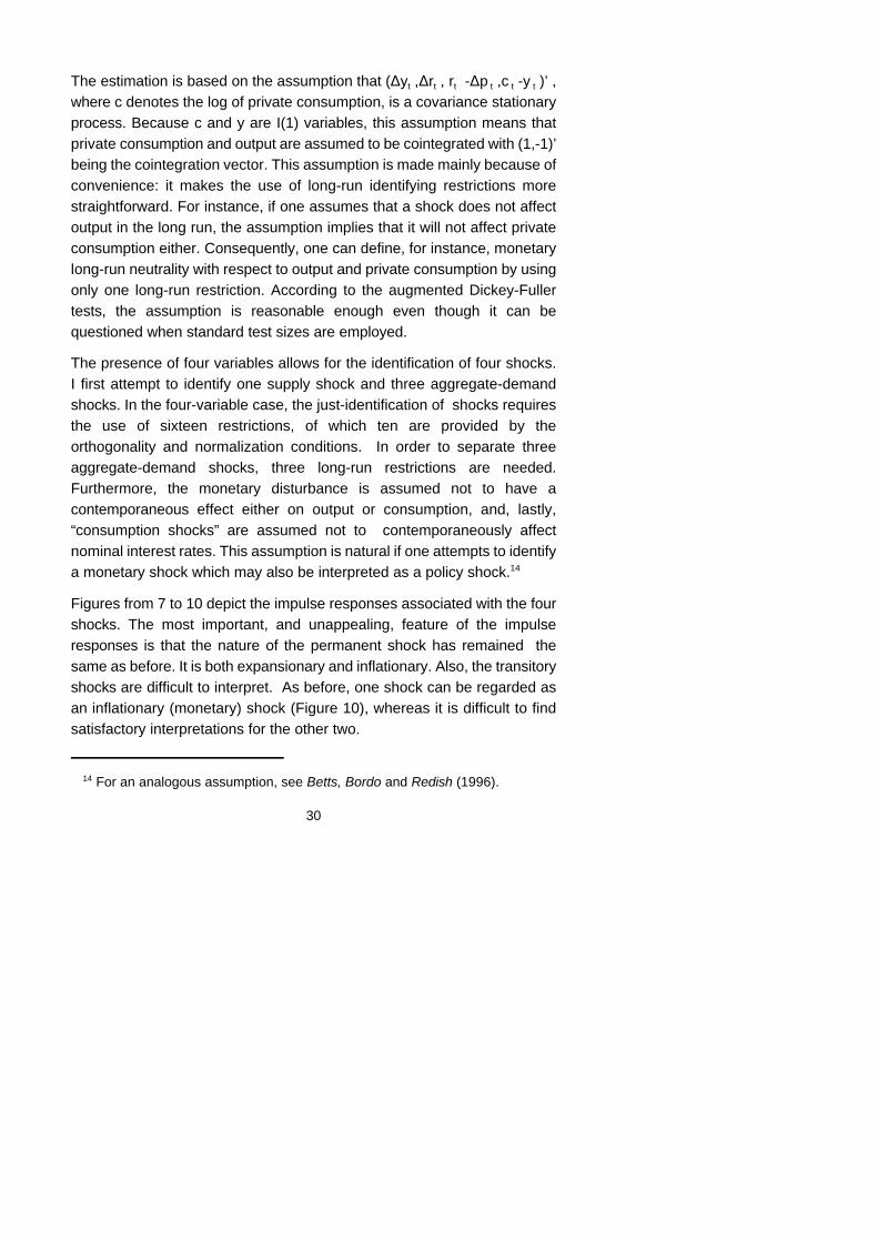
Figures 11 and 12 display the relevant impulse responses when D equalsunity. (Figure 11 is analogous to Figure 7, and Figure 12 to Figure 8.) Thepatterns in Figures 7 and 11 are similar, even though the shock in Figure 11seems to be more inflationary. It looks like an aggregate-demand shock,which has a permanent influence on output. The main difference betweenFigures 8 and 12 is that the shock in Figure 12 is expansionary. It is notimpossible to interpret it as an aggregate-supply shock, because, at leastinitially, it has a deflationary impact on the economy. Yet in the longer runit is inflationary.

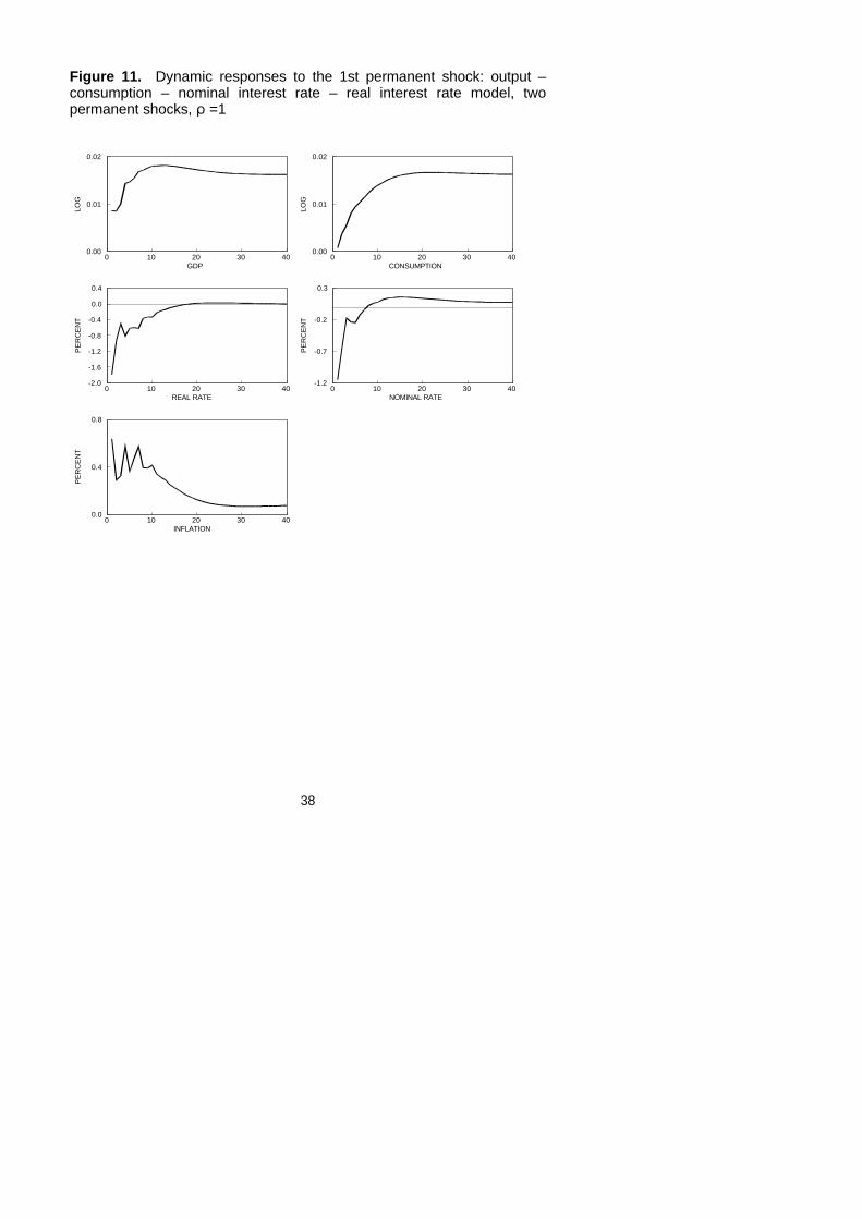
The forecast error decompositions are shown in Table 5. In comparison toTable 3, the importance of the first permanent shock decreases at the costof the second permanent shock. At shorter horizons the first permanentshock is, however, more important than the second one. In the long runthey are, by definition, of equal importance.

Furthermore, at a very short run (contemporaneously) 98.5 per cent of theforecast error variance for private consumption is accounted for by thesecond permanent shock. On the other hand, the first permanent shock isthe most important source of fluctuations in the real interest rate both atshorter and longer horizons. (Tables of these decompositions are availableupon request.)

38

Figure 11. Dynamic responses to the 1st permanent shock: output –consumption – nominal interest rate – real interest rate model, twopermanent shocks, D =1

0 10 20 30 40GDP

0.00

0.01

0.02

LOG


0.00

0.01

0.02

LOG

0 10 20 30 40REAL RATE

-2.0

-1.6

-1.2

-0.8

-0.4

0.0

0.4

PE

RC

EN

T


-1.2

-0.7

-0.2

0.3

PE

RC

EN

T


0.0

0.4

0.8

PE

RC

EN

T

39

Figure 12. Dynamic responses to the 2nd permanent shock: output –consumption – nominal interest rate – real interest rate model with twopermanent shocks, D =1

0 10 20 30 40GDP

0.00

0.01

0.02

LOG


0.00

0.01

0.02

LOG

0 10 20 30 40REAL RATE

-0.5

0.0

0.5

PE

RC

EN

T


-0.1

0.2

0.5

PE

RC

EN

T


-0.6

0.0

0.6

PE

RC

EN

T

40

Table 5. Forecast-error variance decompositions for GDP: output –consumption – nominal interest rate – real interest rate model, twopermanent shocks, D = 1

Horizon in quarters 1st permanentshock

2nd permanentshock

Transitoryshocks


50.855.658.758.156.955.854.851.1

14.832.036.539.241.342.944.148.7

34.412.4 4.8 2.7 1.8 1.3 1.1 0.2


The historical forecast error decompositions are shown in Table 6. It clearlydiffers from Table 4 because of the important role of the secondpermanent shocks. According to Table 6, the boom was caused by asequence of those shocks. During the depression both permanent shocksplayed a major role. The first permanent shock was the most important oneat the early stage of the depression, while the second shock was the mostimportant cause of the prolongation of the depression. Transitory shocksplayed only a minor role both during the boom and the depression.

Table 6 obviously, provides an alternative shock interpretation for both theboom and the depression. But what are the two permanent shocks?

If one adheres to the vertical Phillips curve paradigm, both of them shouldbe interpreted as aggregate supply shocks. But if one takes the patterns ofthe impulse response functions seriously, it is impossible to regard both ofthem as supply shocks. The only way of proceeding, I think, is to take themseriously, and to try to construct an account of the boom and thedepression which is consistent with the shocks.

41

Table 6. Decomposition of eight-quarter forecast errors for GDP: output –consumption – nominal interest rate – real interest rate model,two permanent shocks, D = 1 ( yearly averages for 1986–1995 )

Year GDP 1st permanentshock

2ndpermanent

shock

Transitoryshocks

1986198719881989199019911992199319941995

3.6 2.9 4.9 3.5 -2.5-13.9-12.0 -4.9 1.9 4.5

0.5-1.2-0.1-1.4-4.5-9.2-7.7-0.6 6.4 6.4

2.1 3.9 5.9 5.1 1.3-3.6-3.7-4.1-4.3-2.2

1.1 0.2-0.9-0.2 0.7-1.1-0.6-0.2-0.2 0.3


The first permanent shock is best regarded as an aggregate-demand shock,which affects and operates through the real interest rate. (One transitoryshock also affects the real interest rate but its role is secondary.) Thepositive shock is inflationary and it decreases the real interest rate. Thisdecrease is, however, transitory because acceleration of inflation increasesnominal interest rates. In the long run, the real interest rate returns to itsinitial level.

In addition to the effects of changes in real interest rates, the first shockmay also reflect other factors affecting aggregate-demand. It is highlylikely that, for instance, shocks to export demand are also reflected in thisshock. Table 6 supports this kind of interpretation.

Consistent with the above interpretation, the first shock did not contribute tothe boom. The rise in the real interest rate in 1989 is seen as a negativeshock. The concrete cause of the downturn of the economy, therefore, wasa negative aggregate demand shock operating through the real interest rate

16 Another relevant alternative is to utilize an approach which does not adhere tothe rational choice model. For such an approach, see, for example, Minsky (1986).Meltzer (1995) contains a monetarist approach to the credit channel and to the“credit view”.

42

channel. Yet GDP growth was maintained by the second permanentshock. In 1990, the first shock had a strong contractionary effect on output.The collapse of the Soviet trade is very likely one reason for the very bignegative shock in 1991. The first shock had a small negative effect in 1993,but the recovery of the economy was attributed to it. This is consistent withthe view that changes in the real interest rate and exports are reflected inthe first permanent shock.

As has already become evident, the second permanent shock is not easilyinterpretable. In the very short run, at a six months horizon, it behaves likea supply shock. It is deflationary, and causes a decrease in the nominal rateand an increase in the real rate. In the longer run, the shock is inflationary,however. Except for the very short run, it is an important cause of outputfluctuations. Because it is the main cause of fluctuations in privateconsumption in the short run, it can be called a consumption shock. Alongwith the first permanent shock, it is important in explaining movements inprivate consumption also in the long run. Unlike the first permanent shockit does not seem to be an important factor behind movements in the realinterest rate.

The sequence of the second permanent shocks is consistent with theinterpretation, which emphasises the role of credit and the credit channel.One can, of course, give many rationalizations for the sequence of thesecond permanent shocks, each highlighting the role of credit and the creditchannel. If one does not want to assume irrational behaviour by privateeconomic agents, one can attempt to utilize the economics of imperfectinformation and the (new Keynesian) “credit view” which is built on thatliterature. This is, of course, only one alternative.16

The “credit view” underlines the role of two channels, the balance sheetchannel and the bank lending channel, in the propagation of monetary

17 In this paper, the role of private consumption and households is stressed, andperhaps even exaggerated, at the cost of private investment and firms. For ananalogous emphasis, see Mishkin (1978).

43

policy measures (see, for instance, Bernanke and Gertler, 1995).Obviously, both of these channels played an important role in the boom,which was accompanied with credit explosion. During the boom they werean essential part of the mechanism which boosted GDP growth, whileduring the depression the two channels played an adverse role.

The sequence of the second permanent shocks can be interpreted asmainly reflecting the expansionary and contractionary roles of these twochannels first of all for the development of private consumption.17

Table 6 shows that the role of the second permanent shock was notimportant at the outset of the depression, but it contributed to the depth ofthe depression, and, what is most important, to the length of thedepression. GDP started to rise in 1994 but the second shock had acontractionary effect as late as in 1995. For the depression years, thesequence of the second permanent shocks can be interpreted as describingthe debt-deflation process during which both the balance sheet channel andbank lending channel were important.

When explaining the length of the Great Depression both Cecchetti andKarras (1994), and Betts, Bordo and Redish (1996) utilized Bernanke’s(1983) theory of the collapse of financial intermediation. It emphasizes therole of the bank lending channel. Bernanke argues, resting on the “creditview”, that the main reason for the lengthening of the Great Depression wasan increase in the cost of financial intermediation, which resulted in a largenumber of otherwise creditworthy borrowers being denied loans. Theincrease was a risk premium demanded by risk-averse bankers.

In both Cecchetti and Karras (1994), and Betts, Bordo and Redish (1996)the negative supply shocks, which were associated with the prolongation ofthe Great Depression, are interpreted as reflecting the collapse of financialintermediation.

18 Vihriälä’s (1997) study of the Finnish banking crisis is based on the “creditview”. According to Vihriälä (1997), the moral hazard of weak banks played a rolein the expansion phase, and insufficient capital constrained lending later. Creditcontraction was caused rather by ’collateral squeeze’ than by ’credit crunch’.

44

A similar interpretation can be given for the sequence of the secondpermanent shocks. In additon to borrowers’ need to adjust their balancesheets, the Finnish banking crisis, which led to credit contraction, providesone rationalization for negative shocks in 1994 and 1995.18

According to the impulse response functions, it is not obvious that thesecond shock should be regarded as an aggregate-supply shock. This is,however, not inconsistent with the “credit view” , because the shocks whichoperate through the balance sheet channel and the bank loan channel mayaffect both aggregate-supply and aggregate-demand.

The above experiment shows that, also within the traditional aggregate-demand – aggregate-supply framework, it is possible to produce resultswhich emphasize the role of private consumption, and the credit channel.Furthermore, they are consistent with the debt-deflation interpretation aboutthe depression.

Yet the results are not robust. It is possible to generate shocks which arevery difficult to interpret and which therefore do not support any of thevarious explanations of the causes of the depression

Obviously, the traditional aggregate-demand – aggregate-supply modelsare not necessarily very useful when the “credit view” is utilized in theinterpretation of shocks, since credit and the above two channels have noexplicit role in these models. Therefore, one can argue that the reasoning,for instance, in both Cecchetti and Karras (1994) and Betts, Bordo andRedish (1996) was not based on the models the authors employed. Thiskind of criticism applies to this paper, too.

Furthermore, Finland is a special case, because in the interpration of theshocks one should take into account, for instance, the effects of putting anend to credit rationing. Blinder (1987) has developed a model which

19 I will not discuss the effects of terms of trade shocks within an explicit model.For that kind of discussion, see, for instance, Hoffmaister and Roldós (1997).

45

describes an economy suffering, because of credit rationing, from“effective supply failure”. In Blinder’s model, firms must pay their factors ofproduction before they receive revenues from sales, and must borrow inorder to do so. But if they cannot get the credit, they must cut back theirhiring. This causes effective supply failure. Blinder’s model illustrates, eventhough one would not have confidence in its descriptive relevance, why theuse of the standard aggregate-demand – aggregate-supply framework maybe exceptionally problematic in the case of Finland.

External shocks provide an extra difficulty. In the Finnish debate, theimportance of terms of trade shocks have been highlighted by those whoregard the depression as an outcome of negative external shocks (seeTarkka 1994). Consequently, “consumption shocks” may reflect changes inthe terms of trade. In what follows, the validity of this interpration isanalysed by adding the terms of trade variable into the above four-variablemodel.19

A five-variable model: the role of the terms of trade

Even though all of the above results have not been robust, the importantrole of permanent shocks, whether they are aggregate-demand oraggregate-supply shocks, has been a permanent feature. Onemanifestation of the non-robustness of the results was that it wasimpossible to give a robust interpretation for the permanent shocks.Analysing the role of terms of trade can help identify these shocks,perhaps by ruling out some interpretations.

I estimate a five-variable VAR model which includes the terms of tradevariable, tot, as one variable. The model is based on the assumption that()tott, )yt ,)p t ,r t -)p t ,c t -y t )’ is a stationary process. This means that the

46

terms of trade are assumed to be an I(1) variable. This assumption isconsistent with standard ADF tests.

Furthermore, according to block exogeneity tests, there is no need toinclude the other variables in the autoregression for the terms of trade. Itcan be regarded as an exogenous variable with respect to the othervariables. Therefore, the unconstrained reduced form is estimated underthis assumption, which implies that the analysis is based on the estimationof a near VAR model.

The identification of shocks is a straightforward generalization of theBlanchard-Quah (1989) identification. Just-identification requires the use oftwenty-five constraints, of which fifteen are given by the orthogonality andnormalization conditions. In addition to those constraints, three long-runconstraints are imposed in order to separate three transitory shocks whichdo not affect output in the long-run. This means that two permanent shocks,of which one is a terms of trade shock, are identified. I assume that theother four shocks do not affect the terms of trade contemporaneously. Thisassumption provides four short-run restrictions. The last three equations areanalogous to those used within the four-variable model. One transitoryshock, the “monetary shock”, does not contemporaneously affect outputand consumption. This gives two restrictions. The last assumption is thatone of the other two transitory shocks does not contemporaneously affectnominal interest rates.

The importance of the terms of trade shocks can be assessed by forecast-error variance decompositions and historical forecast error decompositions.

Table 7 shows that about ten per cent of the output variability is accountedfor by terms of trade shocks at the business cycle frequencies. Hence,terms of trade shocks are a noteworthy source of output fluctuations buttheir importance should not be exaggerated. As a source of fluctuations inprivate consumption their importance is even somewhat greater. Atbusiness cycle frequencies about twenty per cent of the forecast errorvariance is accounted for by terms of trade shocks. (This table is availableupon request.)

47

Yet according to the historical forecast-error compositions (Table 8), termsof trade shocks did not play a decisive role either during the boom or duringthe depression. Their relative importance was greatest at the start of the

48

Table 7. Forecast-error variance decompositions for GDP: terms of trade –output-consumption – nominal interest rate – real interest rate model, twopermanent shocks

Horizon in quarters Terms of trade shock

2nd permanentshock

Transitoryshocks


0.6 8.4 9.2 9.4 9.810.310.813.2

28.055.371.878.781.883.384.085.5

71.436.319.011.8 8.3 6.4 5.2 1.3


Table 8. Decomposition of eight-quarter forecast errors for GDP: terms oftrade – output-consumption – nominal interest rate – real interest ratemodel, two permanent shocks (yearly averages for 1986–1995)

Year GDP Terms oftrade shock

2nd permanent shock

Transitoryshocks

1986198719881989199019911992199319941995

3.4 3.0 4.6 3.4 -2.7-14.0-11.6 -4.9 1.9 4.6

0.3 1.1 0.8 0.8 0.2-0.5-0.5-0.4-0.3 0.7

2.4 2.7 5.6 3.8 -3.0-11.8-10.1 -5.1 1.0 2.8

0.7-0.8-1.8-1.1 0.1-1.7-1.0 0.6 1.2 1.1


49

boom in 1987. During the depression, the worsening of the terms of tradeplayed only a minor role.

These results, therefore, do not support the view that terms of trade shockswere an important factor contributing both to the boom and the depression.The results are in contrast with the third interpretation of the depression.The bulk of the fluctuations is explained by other permanent shocks. Unlikemost of the previous conclusions and interpretations, this conclusion isbased on a model within which the shock, the terms of trade schock, waswell-identified.

50

5. CONCLUSIONS

The main aim of this paper was to explore the boom and the depression byestimating structural VAR models which are based, first of all, on theutilization of the traditional aggregate-demand – aggregate-supplyframework. Typically, these models belong to the class of IS-LM models,which have been augmented with a Phillips curve.

This paper attempted to deepen the exploration initiated in Sauramo(1996) by linking the econometric investigation more closely to economictheory. One can expect that the use of the aggregate-demand – aggregate-supply framework is superior to largely atheoretic frameworks such as theones utilized in Blanchard (1993) or Sauramo (1996), since theinterpretation of shocks should become easier.

However, the usefulness of that kind of investigation crucially depends onhow well the framework fits the data. For Finland, finding a suitableframework is far from obvious. Until the mid eighties, the financial marketswere regulated and therefore the standard textbook versions were more orless inapplicable in the description of the behaviour of the economy. Thederegulation of the financial markets has brought about a drastic change,but this does not necessarily make the analysis easier: institutionalchanges were accompanied by shifts in the exchange rate policy andmonetary policy regimes, which complicates the use of the standard IS-LMframework or the Mundell-Fleming framework.

The identification of shocks which would be compatible with the standardframework turned out to be difficult. For instance, most of the permanentshocks which were identified looked more like aggregate-demand thanaggregate-supply shocks. Furthermore, identifying monetary policy shocksturned out to be impossible. In fact, if one takes into account the above

51

changes in the institutional environment, this is what one would expect.Endogenous changes dominate the relevant policy variables.

Despite all these difficulties, the analysis provided some noteworthy results.

The bulk of output fluctuations are explained by permanent shocks. Exceptfor the very short run (one to four quarters), transitory shocks are of minorimportance. Even though this result is related to the difficulty to identifyrelevant transitory shocks, the major role of permanent shocks may havebeen an essential characteristic of output fluctuations in Finland.

It was the identification of permanent shocks which was the most importantand difficult part of the investigation. The considerations which were basedon the assumption about the vertical long-run Phillips curve were largelycounterproductive. If only one permanent shock was allowed to exist itlooked more like an aggregate-demand than an aggregate-supply shock.Perhaps the most appealing results were obtained when, within a four-variable model, two permanent shocks were assumed to exist, and theassumption about the vertical long-run Phillips curve was relaxed. In thatcase, the two permanent shocks could be given reasonable interpretations.One was an aggregate-demand shock causing changes in the real interestrate and also reflecting other factors affecting aggregate-demand, inparticular, export demand. The other one could be interpreted as a supplyshock, even though it was inflationary in the longer run. I regarded it as ashock which operates mainly through the credit channel. It was a shockwhich explained the boom of the late eighties and, in particular, the lengthof the depression. These results were consistent with the debt-deflationinterpretation of the depression.

The identification of the above two permanent shocks was, however, notrobust. Therefore these results could have been more persuasive. On theother hand, the validity of the third interpretation about the causes of thedepression was assessed by analysing the role of the terms of trade. Theresults contrasted with the view that adverse shocks to the terms of tradeplayed a major role in the birth of the depression. This outcome wasunrelated to the non-robust identification.

20 For an appealing framework for estimating technology shocks, see Gali(1996).

21 Furthermore, the traditional aggregate-demand – aggregate-supply frameworkhas been criticised as being logically inconsistent. See, for instance, Barro (1994),Colander (1995), and Hall and Threadgold (1982). Even though this criticism is

52

According to Sauramo (1996) the main “cause” of the boom and thedepression were positive and negative “consumption shocks”. The issue leftunanswered was what these shocks are. In this paper this issue has beenanalysed within the traditional aggregate-demand – aggregate-supplyframework. Even though the results do not provide a persuasive answer tothis question they do support the view that it is very difficult to give a goodexplanation of the causes of the depression by ignoring the credit channel,and the (policy) measures which have operated through it.

The analysis of this paper has still been tentative, and it may raise morequestions than it answers. Perhaps the most puzzling, and robust, featureof the results was that they could not be reconciled with the vertical long-run Phillips curve paradigm. On the contrary, they were consistent with theview that GDP growth has largely been determined by aggregate-demand.This may be the case, and there are good arguments which support thisview. Yet one can make progress in identifying aggregate-supply shocks.For example, the identification of technology shocks would be a naturalextension of the analysis of this paper. The identification of technologyshocks may help to solve some of the puzzles raised by this paper.20

But it is unlikely to provide a solution to the problem associated with theinterpretation and identification of “consumption shocks”. Cochrane (1994)argues that the puzzle of “consumption shocks” may remain unsolved, if“consumption shocks” reflect news that agents see but we do not, andcontinues: “If this view is correct, we will forever remain ignorant of thefundamental causes of economic fluctuations.” (See the abstract of thepaper.) This comment strongly motivates further research. According to thispaper, one should be ready to rely on the frameworks which are not basedon the vertical long-run Phillips curve paradigm.21

aimed at some conventional theoretical models, econometric models which utilizethese models are not immune to it. This gives an additional reason for the use offrameworks other than the traditional aggregate-demand – aggregate-supplyframework.

53

REFERENCES

Ahtiala, P. (1997), Economic Policy and the Depression, Finnish EconomicJournal 1/1997, 61–85 (in Finnish).

Barro, R. J. (1994), The Aggregate-Supply/Aggregate-Demand Model,Eastern Economic Journal, 20, 1–6.

Bayoumi, T. and B. Eichengreen (1994), One Money or Many? Analyzingthe Prospects for Monetary Unification in Various Parts of the World,Princeton Studies in International Finance, No. 76, New Jersey.

Bergman, M. (1992), Essays on Economic Fluctuations, Lund EconomicStudies number 51, Malmö 1992.

Bernanke, B. (1983), Nonmonetary Effects of the Financial Crisis in thePropagation of the Great Depression, American Economic Review, 73,257–276.

Bernanke, B. and A. Blinder (1988), Credit, Money, and AggregateDemand, American Economic Review, 78, 435–439.

Bernanke, B. and A. Blinder (1992), The Federal Funds Rate and theChannels of Monetary Transmission, American Economic Review, 82,901–921.

Bernanke, B. and M. Gertler (1995), Inside the Black Box: The CreditChannel of Monetary Policy Transmission, Journal of EconomicPerspectives,9, 27–48.

54

Betts, C. M., M. D. Bordo and A. Redish (1996), A Small Open Economy inDepression: Lessons from Canada in the 1930s, Canadian Journal ofEconomics, 29, 1–36.

Blanchard. O. J. (1993), Consumption and the Recession of 1990–1991,American Economic Review 83, 270–274.

Blanchard, O. J. and D. Quah (1989), The Dynamic Effects of AggregateDemand and Supply Disturbances, American Economic Review, 79, 655–673.

Blinder, A. (1987), Credit rationing and effective supply failures, EconomicJournal, 97, 327–353.

Bordes, C., D. Currie and H. T. Söderström (1993), Three Assessments ofFinland’s Economic Crisis and Economic Policy, Bank of Finland C:9,Helsinki.

Brunner, K. (ed.)(1981), The Great Depression Revisited, New York.

Brunner, K. and A. H. Meltzer (1988), Money and Credit in the MonetaryTransmission Process, American Economic Review, 78, 446–451.

Cecchetti, S. G. and G. Karras (1994), Sources of Output FluctuationsDuring the Interwar Period: Further Evidence on the Causes of the GreatDepression, The Review of Economics and Statistics, 76, 80–102.

Cochrane, J. H. (1994), Shocks, Carnegie-Rochester Conference Series onPublic Policy, 41, 295–364.

Colander, D. (1995), The Stories We Tell: A reconsideration of AS/ADAnalysis, Journal of Economic Perspectives, 9, 169–188.

Erkel-Rousse, H. and J. Melitz (1995), New empirical evidence on the costsof European Monetary Union, Document de travail no 9516, INSEE, Paris.

Fisher, I. (1932), Booms and Depressions, New York, 1932.

Fisher, I. (1933), The Debt-Deflation Theory of Geat Depressions,Econometrica , 1, 337–357.

55

Fisher, L. A., P. L. Fackler and D. Orden (1995), Long-run identifyingrestrictions for an error-correction model of New Zealand money, prices andoutput, Journal of International Money and Finance, 14, 127–147.

Gali, J. (1992), How Well Does the IS-LM Model Fit Postwar U. S. Data?Quarterly Journal of Economics, 107, 709–738.

Gali, J. (1996), Technology, Employment, and the Business Cycle: DoTechnology Shocks Explain Aggregate Fluctuations? NBER Working PaperNo. 5721.

Gerlach, S. and J. Klock (1991), Supply and demand disturbances andSwedish business cycles 1864–1988, Skandinaviska Enskilda BankenQuarterly Review 1–2, 1991, 33–42.

Gerlach, S. and F. Smets (1995), The Monetary Transmission Mechanism:Evidence from the G-7 countries, CEPR Discussion Paper No. 1219,London.

Hall, P. H. and M.L. Threadgold (1982), Aggregate Demand Curves: AGuide to Use and Abuse, Australian Economic Papers, 21, 37–48.

Hartikainen, J. (1995), Dynamic Effects of Demand and SupplyDisturbances on the Finnish Economy: Did Liberalization of CapitalMovements Matter? Bank of Finland Discussion Papers 36/95. Helsinki.

Hoffmaister, A. W. and J. E. Roldós (1997), Are Business Cycles Differentin Asia and Latin America?, International Monetary Fund, WP/97/9.Washington.

Kukkonen, P. (1997), Monetary Policy and the Finnish Economic Crisis,Reports and Discussion Papers No. 149, Pellervo Economic ResearchInstitute, Helsinki (in Finnish).

Mellander, E., A. Vredin and A. Warne (1990), Stochastic Trends andEconomic Fluctuations in Small Open Economies: The Cases of Finlandand Sweden, Working Paper No. 82, Trade Union Institute for EconomicResearch, Stockholm.

56

Meltzer, A. H. (1995), Monetary, Credit and (Other) TransmissionProcesses: A Monetarist Perspective, Journal of Economic Perspectives,9, 49–72.

Minsky, H. (1986), Stabilizing an Unstable Economy, New York.

Mishkin, F. S. (1978), The Household Balance Sheet and the GreatDepression, Journal of Economic History, 38, 918–937.

Sauramo, P. (1991), Blood, Sweat and Tears – Why?, Finnish EconomicJournal 4/1991, 469–480 (in Finnish).

Sauramo, P. (1996), The Boom and the Depression – A Simple ShockInterpretation, Discussion papers 132, Labour Institute for EconomicResearch, Helsinki.

Schön, E. (1995), Business Cycles in an Open Economy Framework:Balancing Economeric Tools and Economic Models, (mimeo) Geneva.

Shapiro, M. D. and M. W. Watson (1988), Sources of Business CycleFluctuations, in Fischer, S. (ed). NBER Macroeconomics Annual 1998,Cambridge, MA.

Sims, C. (1992), Interpreting the Macroeconomic Time Series Facts: TheEffects of Monetary Policy, European Economic Review, 36, 975–1011.

Sterne, G. and T. Bayoumi (1993), Temporary Cycles or Volatile Trends?Economic Fluctuations in 21 OECD Economies, Working Papers No 13,Bank of England, London.

Strongin, S. (1995), The Identification of Monetary Policy Disturbances:Explaining the Liquidity Puzzle, Journal of Monetary Economics, 35, 463–498.

Söderström, H. T. (1993), Finland’s Economic Crisis: Causes, PresentNature, and Policy Options, in Bordes, Currie and Söderström (1993).

Tarkka, J. (1994), The Importance of External Factors in the FinnishEconomic Crisis, Finnish Economic Journal 1/1994, 5–17 (in Finnish).

57

Vihriälä, V. (1997), Banks and the Finnish Credit Cycle 1986–1995, Bank ofFinland Studies E:7, Helsinki.

Government & Nonprofit

The Boom and the Depression: An Analysis within the Aggregate-Demand - Aggregate-Supply Framework