Statistics “Two”Mohamed Ahmed Hefny, MD.

Describing Data with Tables

Learning objectives

At the end of this lecture, you should be able to:

• Explain what a frequency distribution is.• Construct a frequency table from raw data.• Construct relative frequency, cumulative frequency and relative

cumulative frequency tables.• Construct grouped frequency tables.• Construct a cross-tabulation table.• Explain what a contingency table is.• Rank data.

Frequency tables Nominal data

Frequency tables – nominal data

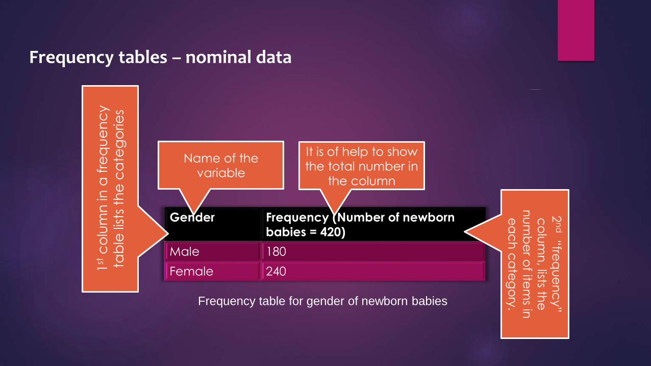
Gender Frequency (Number of newborn

babies = 420)

Male 180

Female 240

Name of the

variable

1st

co

lum

n in

a f

req

ue

nc

y

tab

le li

sts

the

ca

teg

orie

s

It is of help to show

the total number in

the column

2n

d“fre

qu

en

cy”

co

lum

n, lists th

e

nu

mb

er o

f item

s in

ea

ch

ca

teg

ory

.Frequency table for gender of newborn babies

The frequency distribution

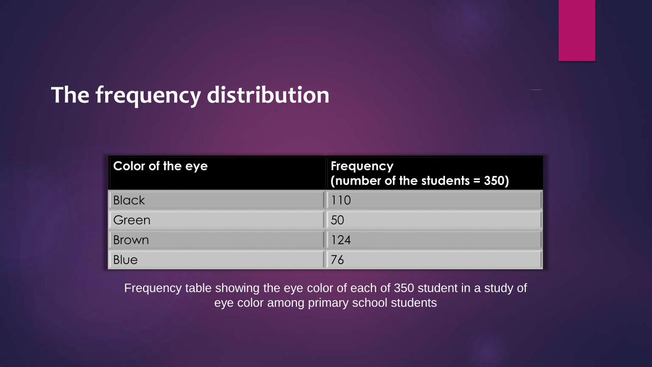
Color of the eye Frequency

(number of the students = 350)

Black 110

Green 50

Brown 124

Blue 76

Frequency table showing the eye color of each of 350 student in a study of

eye color among primary school students

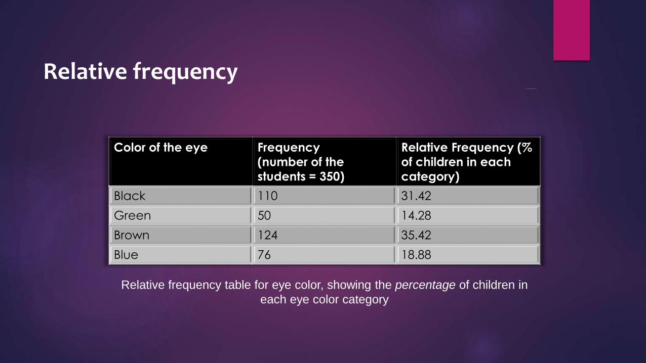
Relative frequency

Color of the eye Frequency

(number of the

students = 350)

Relative Frequency (%

of children in each

category)

Black 110 31.42

Green 50 14.28

Brown 124 35.42

Blue 76 18.88

Relative frequency table for eye color, showing the percentage of children in

each eye color category

Frequency tables Ordinal data

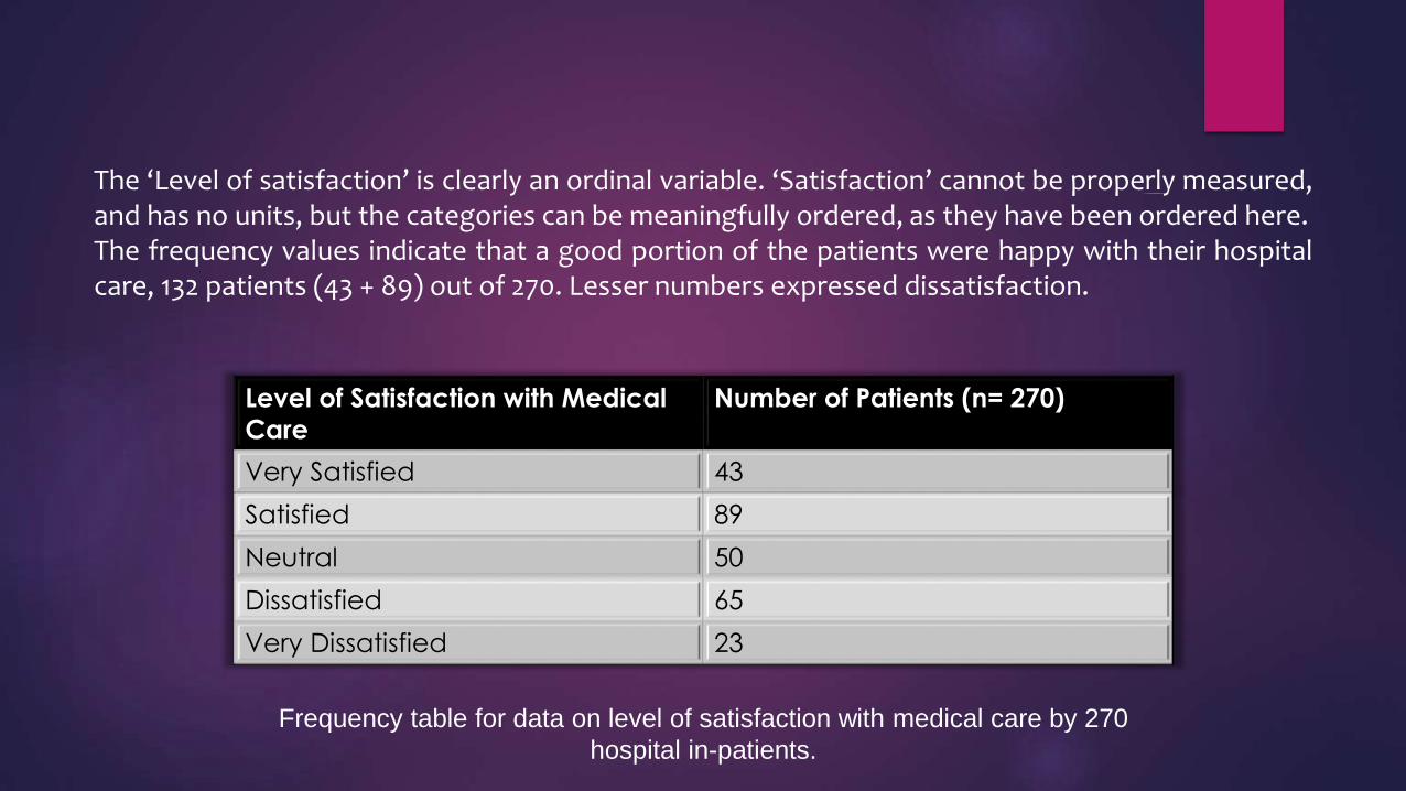
Level of Satisfaction with Medical

Care

Number of Patients (n= 270)

Very Satisfied 43

Satisfied 89

Neutral 50

Dissatisfied 65

Very Dissatisfied 23

Frequency table for data on level of satisfaction with medical care by 270

hospital in-patients.

The ‘Level of satisfaction’ is clearly an ordinal variable. ‘Satisfaction’ cannot be properly measured,and has no units, but the categories can be meaningfully ordered, as they have been ordered here.The frequency values indicate that a good portion of the patients were happy with their hospitalcare, 132 patients (43 + 89) out of 270. Lesser numbers expressed dissatisfaction.

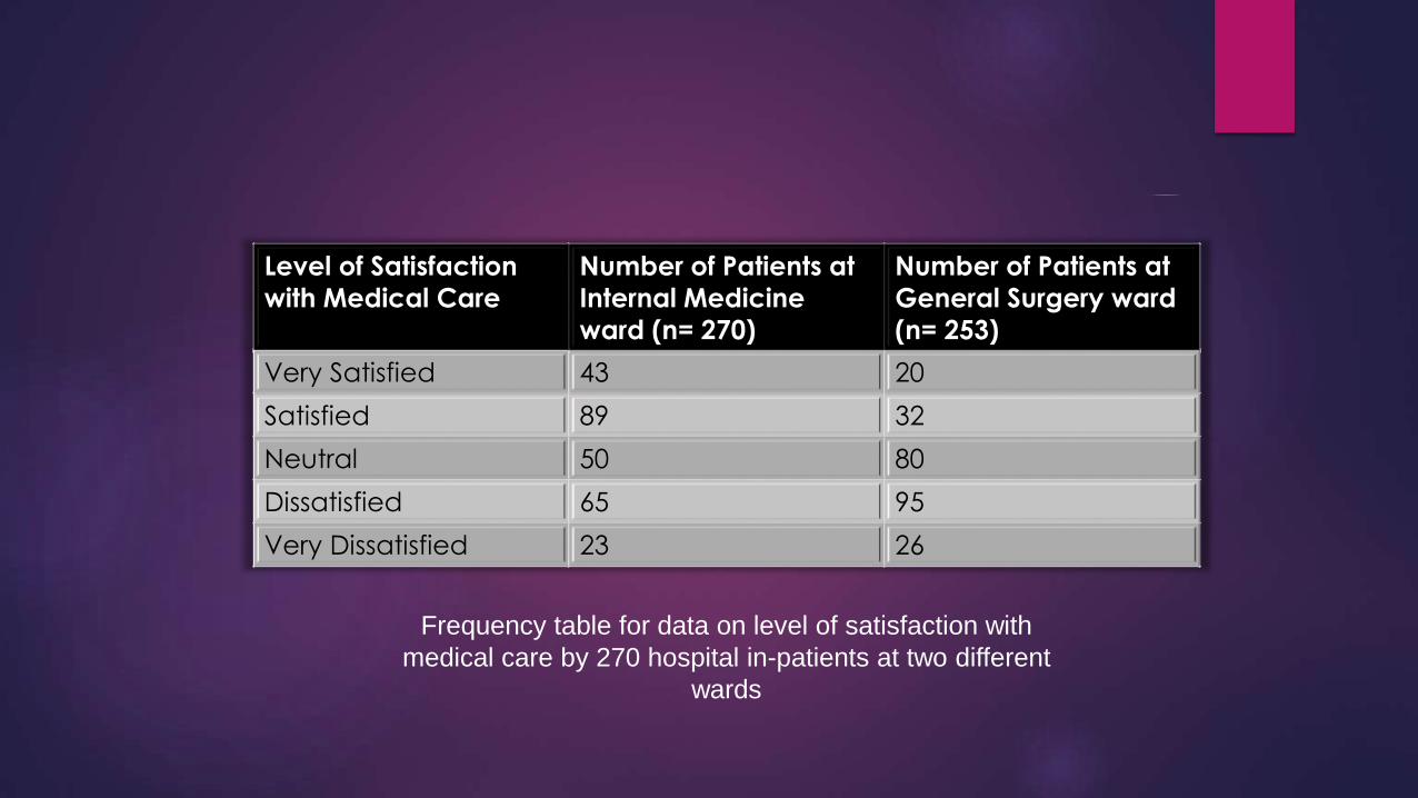
Level of Satisfaction

with Medical Care

Number of Patients at

Internal Medicine

ward (n= 270)

Number of Patients at

General Surgery ward

(n= 253)

Very Satisfied 43 20

Satisfied 89 32

Neutral 50 80

Dissatisfied 65 95

Very Dissatisfied 23 26

Frequency table for data on level of satisfaction with

medical care by 270 hospital in-patients at two different

wards

Frequency tables Metric data

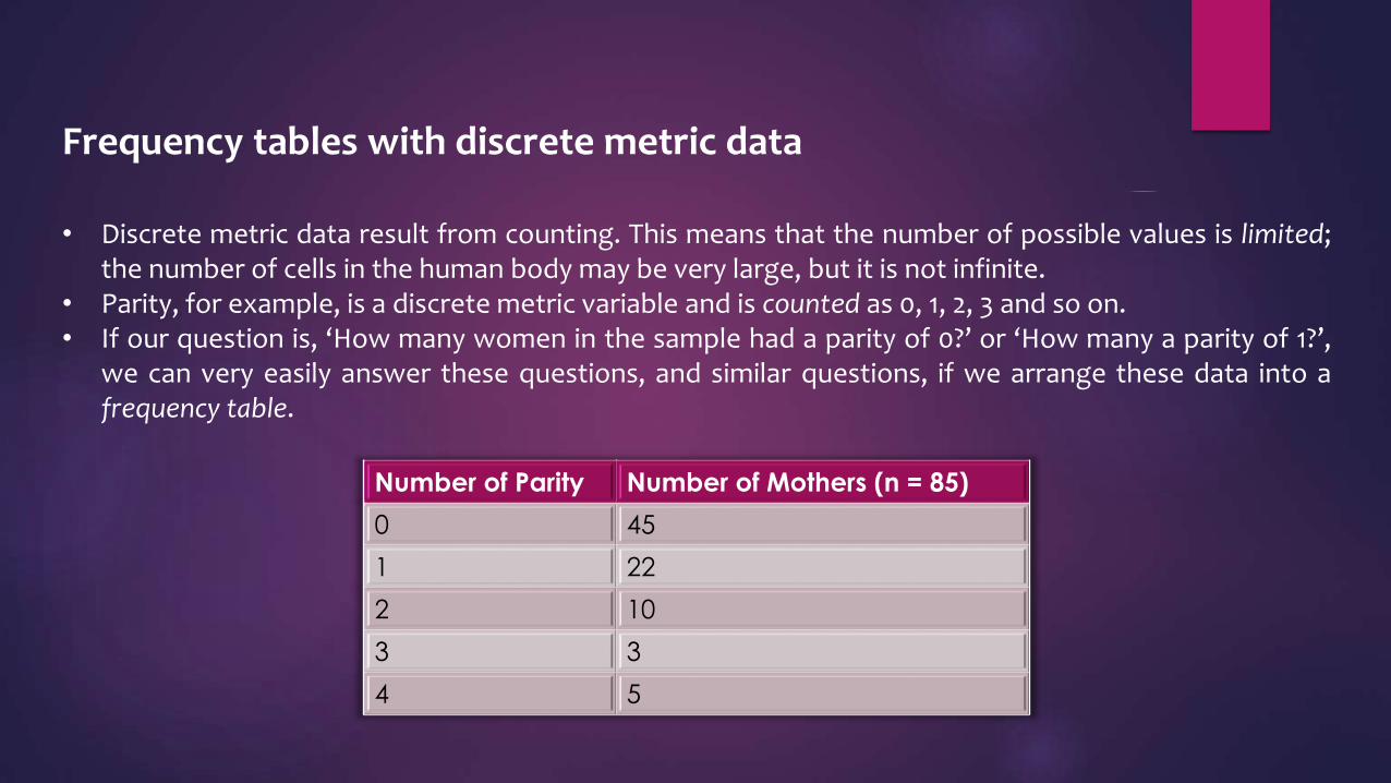
Frequency tables with discrete metric data

• Discrete metric data result from counting. This means that the number of possible values is limited;the number of cells in the human body may be very large, but it is not infinite.

• Parity, for example, is a discrete metric variable and is counted as 0, 1, 2, 3 and so on.• If our question is, ‘How many women in the sample had a parity of 0?’ or ‘How many a parity of 1?’,

we can very easily answer these questions, and similar questions, if we arrange these data into afrequency table.

Number of Parity Number of Mothers (n = 85)

0 45

1 22

2 10

3 3

4 5

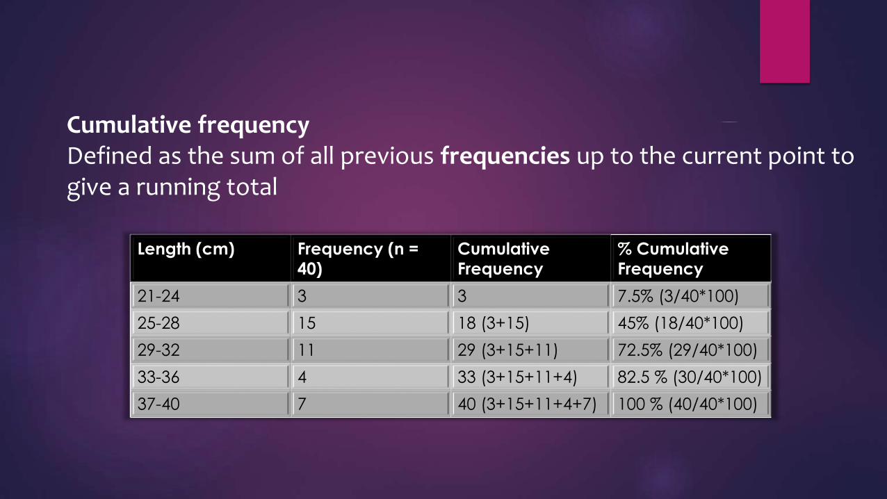
Cumulative frequencyDefined as the sum of all previous frequencies up to the current point to give a running total

Length (cm) Frequency (n =

40)

Cumulative

Frequency

% Cumulative

Frequency

21-24 3 3 7.5% (3/40*100)

25-28 15 18 (3+15) 45% (18/40*100)

29-32 11 29 (3+15+11) 72.5% (29/40*100)

33-36 4 33 (3+15+11+4) 82.5 % (30/40*100)

37-40 7 40 (3+15+11+4+7) 100 % (40/40*100)

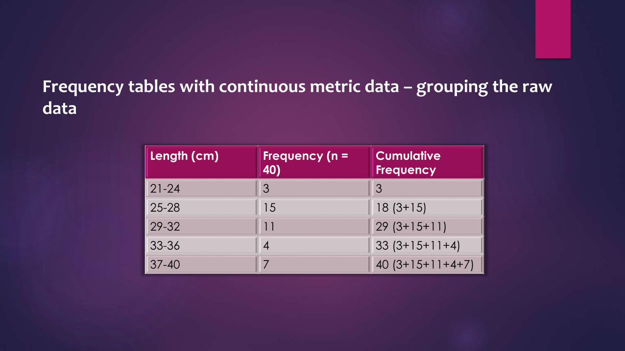
Frequency tables with continuous metric data – grouping the raw data

Length (cm) Frequency (n =

40)

Cumulative

Frequency

21-24 3 3

25-28 15 18 (3+15)

29-32 11 29 (3+15+11)

33-36 4 33 (3+15+11+4)

37-40 7 40 (3+15+11+4+7)

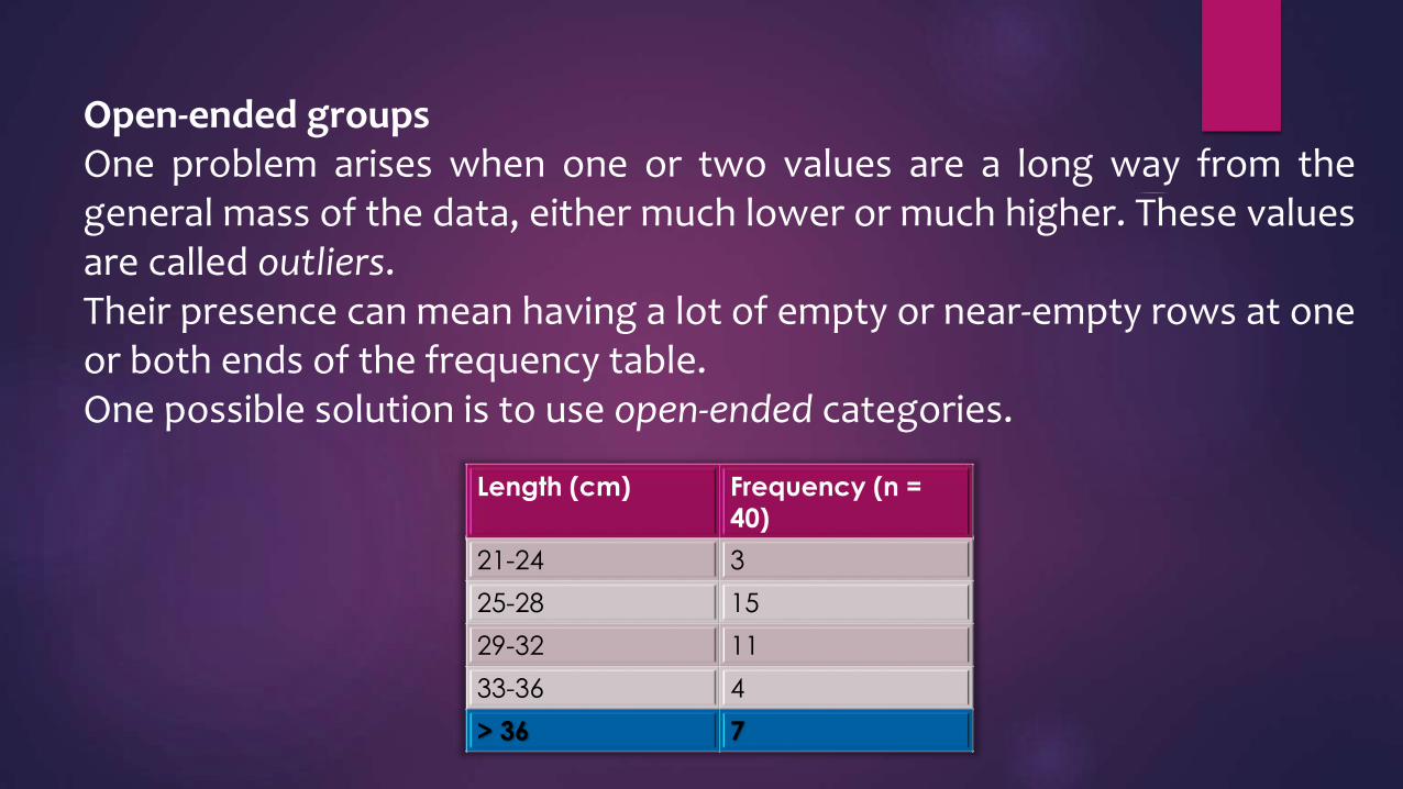
Open-ended groupsOne problem arises when one or two values are a long way from thegeneral mass of the data, either much lower or much higher. These valuesare called outliers.Their presence can mean having a lot of empty or near-empty rows at oneor both ends of the frequency table.One possible solution is to use open-ended categories.

Length (cm) Frequency (n =

40)

21-24 3

25-28 15

29-32 11

33-36 4

> 36 7

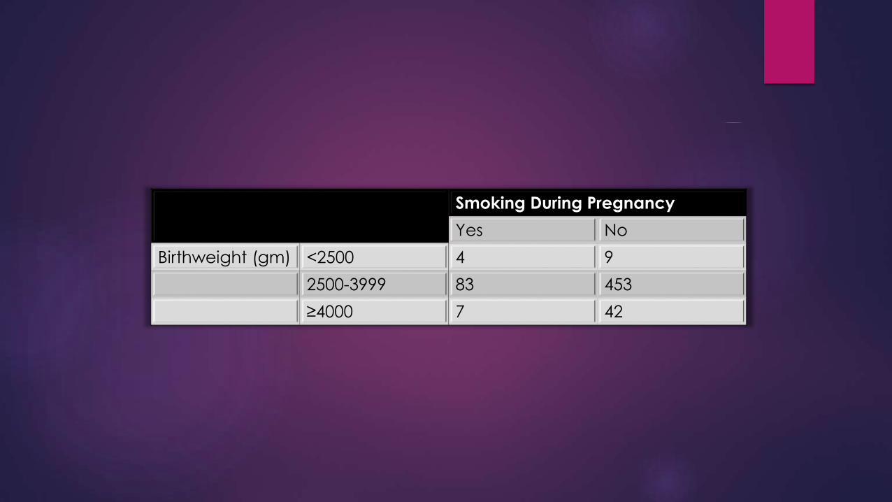
Cross-tabulation – contingency tables

• Sometimes, however, you will want to examine the associationbetween two variables, within a single group of individuals.

• It can be done by putting the data into a contingency table, also calleda table of cross-tabulations.

• In these tables, the rows represent the categories of one variable,usually an ‘outcome’ of some sort (e.g. a diagnosis of lung cancer –Yes or No), and the columns represent the groups within a secondvariable (e.g. smokers and non-smokers)

Smoking During Pregnancy

Yes No

Birthweight (gm) <2500 4 9

2500-3999 83 453

≥4000 7 42

Thank You