Electronic copy available at: http://ssrn.com/abstract=2698157

VOTER PREFERENCES AND POLITICAL CHANGE:

EVIDENCE FROM THE POLITICAL ECONOMY OF SHALE BOOMS

Viktar Fedaseyeu, Bocconi University

Erik Gilje, The Wharton School

&

Philip E. Strahan, Boston College and NBER

November 2015

ABSTRACT

Local interests change sharply after the energy booms that began in 2003, when hydraulic fracturing spurred extraction of formerly uneconomic oil and gas reserves. Support for conservative interests rises and Republican political candidates gain votes after booms, leading to a near doubling in the probability of a change in incumbency. All of this change occurs at the expense of Democrats. Voting records of U.S. House members from boom districts become sharply more conservative across a wide range of issues, including issues unrelated to energy policy. At the level of the individual, marginal candidates skew their voting behavior somewhat toward more conservative causes, but generally not enough to maintain power. Thus, even when the stakes are high and politicians risk losing power, ideology trumps ambition.

Electronic copy available at: http://ssrn.com/abstract=2698157

1. INTRODUCTION

How do changes in electoral preferences translate into changes in political outcomes?

Political theory has contrasted two ways in which a democratic political system might respond to

sharp shifts in voter preferences. At one extreme, electoral competition may force politicians

themselves to alter their voting behavior toward the new median voter’s preferred outcomes

(Downs, 1957; Calvert, 1985). This view implies large changes in the voting behavior of

individual politicians but small changes in election outcomes. At the other extreme, politicians

may hold fast to their ideology, either because of principle or because their past votes make it

hard to credibly commit to voters that they would support different policies (Alesina, 1988).

This alternative would imply large changes in election outcomes but small changes in the voting

behavior of individual politicians. In this paper we design a series of tests to identify how

changes in electoral preferences affect political outcomes.

Identifying the effect of changes in electoral preferences on political outcomes is

empirically challenging, because electoral preferences are not randomly assigned. Any number

of omitted variables could be correlated with both electoral preferences and political outcomes

(e.g. wealth). To make progress towards addressing these endogeneity issues, we focus our

analysis on events that have caused among the largest electoral preference shifts in the last

decade in the American political system: shale discoveries. We use this large and exogenous

shock to voter interests from the shale discoveries of the 2000s to trace out empirically how the

political equilibrium responds. These shocks provide significant variation in electoral

preferences across congressional districts and over time. The booms stem from hydraulic

fracturing (“fracking”), a new technology that allowed energy companies to exploit previously

uneconomic shale oil and gas reserves. Following these shale booms, support for local

1

politicians shifts toward Republican candidates, and the voting behavior of elected politicians

becomes sharply more conservative across a wide range of issues. However, almost all changes

in this voting behavior result from voters electing new politicians: politicians who face sharp

changes in the preferences of their electorate lose their jobs rather than change their votes.

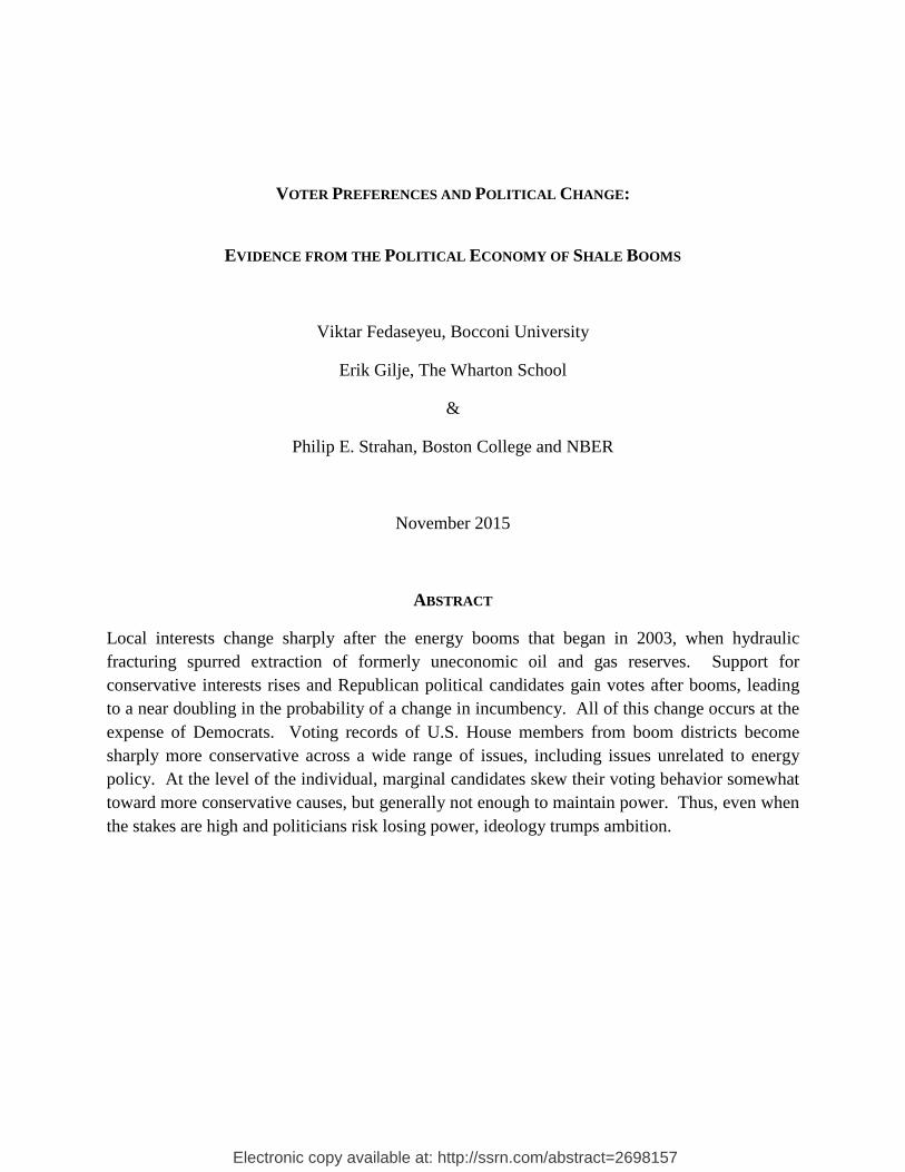
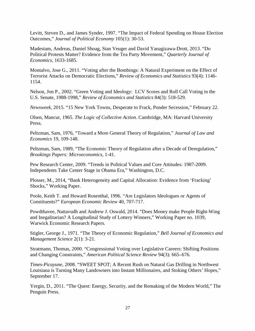
Figure 1 illustrates the magnitude of the electoral shift. We plot over time the share of

Republican House members for Congressional districts that had shale booms, compared with

those never experiencing such booms. The contrast is stark: shale drilling started in 2003, and by

2012 over 80% of House seats were filled by Republicans in boom areas, up from less than 50%

in 1996. In non-shale districts from the same states, however, there is no trend: Republicans

hold about half of the seats across the whole period. On balance, political change associated

with shale development represents among the most significant changes in the U.S. political

system in the last decade. Specifically, shale development is associated with 17 congressional

seats changing control from Democrats to Republicans, accounting for nearly half of the

Republican majority in congress as of 2015.

Our empirical analysis has two components. First, we demonstrate that local support for

Republican candidates increases following shale booms. Focusing on the seven states that have

had large booms, we estimate that the Republican vote share increases in U.S. House elections,

U.S. Senate elections, U.S. Presidential elections, and state gubernatorial elections. In all four

election types, we find conditioning on party matters: the effect is driven by situations in which

the incumbent local office holder is a Democrat, meaning that voters support a switch from a

Democrat to a Republican after booms. And, consistent with these voting patterns, we find that

the probability of a change in incumbency increases sharply following shale booms. The

magnitude of the effect is large economically: overall, when a county moves from its pre-boom

2

to post-boom years, the probability of a change in incumbency rises by 13 percentage points, a

near doubling relative to the unconditional rate of change in incumbency (16 percent). Even

more striking, this result is driven by losses for Democrat incumbents, whose probability of

losing incumbency increases by almost 23 percentage points. We find no effect of shale booms

on incumbency when Republicans hold office.

Second, we analyze interest group ratings at the level of the individual office holder. We

consider the ratings coming from three conservative groups and four liberal groups. The

conservative groups represent business interests (the U.S. Chamber of Commerce), low tax/small

government (the National Taxpayers Union), and conservative causes generally (the American

Conservative Union). The liberal groups represent the interests of labor unions (the Committee

on the Political Education of the AFL-CIO), civil rights (the American Civil Liberties Union),

the environment (the League of Conservation Voters), and liberal causes generally (the

Americans for Democratic Action). Following shale booms, ratings for Congressional office

holders increase from the three conservative groups and decrease from the four liberal ones.

These changes suggest not only that the political interests of the median voter have shifted, but

also that the changes in political attitudes stemming from one kind of shock (energy

development) may spill over into other arenas (civil rights, labor policies, tax policies).

This second approach, which exploits individual rather than geographical data, allows us

to contrast variation at the extensive margin (between office holders) with variation at the

intensive margin (within office holders). The comparison is striking in that almost all of the

changes come at the extensive margin. For example, when we control for individual fixed

effects in our regressions (rather than just geographical effects) there is almost no change in the

voting patterns on either conservative or liberal issues. It is worth emphasizing that this non-

3

result is based not on a lack of statistical power but on big declines in coefficient estimates.

Thus, at least in our setting, ideology trumps ambition.

We also test whether politicians’ voting response to shale booms depends on seniority, on

political party, or on the closeness of prior elections, and find little evidence that it does. One

explanation for a politician’s lack of flexibility stems from reputational lock-in. Having staked

out a certain position, it may be hard or even impossible to signal credibly a change to voters

(Stratmann, 2000). The power of such reputational lock-in ought to grow with seniority. We

report some evidence consistent with this idea, although the estimated interaction between the

advent of booms and seniority on within-individual voting patterns is not robust across

reasonable ways to measure seniority. Neither do we find compelling evidence that Democrats

who survive the shale booms alter their voting behavior. Finally, we find some evidence that

marginal candidates alter their behavior, using the closeness of past elections to isolate

politicians with the greatest incentive to cater to shifting local interests, but again this evidence is

not robust.

Our paper contributes to the debate over the importance of interest groups, institutional

factors and ideology in shaping political outcomes. The interest-group approach emphasizes that

long-run changes in political outcomes depend on the relative strength and bargaining power of

underlying interest groups (e.g., Olsen, 1965; Stigler, 1971; Peltzman 1976, 1989; Irwin and

Kroszner, 1998; Kroszner and Strahan, 1999). Consistent with this view, we find large increases

in the strength of conservative and business interests after the shale booms and a big increase in

support for Republicans, which leads to large changes in incumbency. Thus, changes in the

economic interests of the median voter affect political outcomes because winners of elections

change (the extensive margin).

4

But we also show the importance at the individual level of a fixed ideology that seems to

dominate the voting behavior of politicians. Rather than chase the median voter, they do not

seem to be affected much by changes in the views of their constituencies. At this level, our

results are consistent with Poole and Rosenthal (1996), who emphasize the importance of

ideology, arguing that U.S. Senators from the same state and party often end up on opposite sides

of the same vote. This pattern emerges consistently throughout the history of the U.S. Senate but

is hard to explain based on interest-group factors, since such factors are common for Senators

from the same state and party. Consistent with this view, Levitt (1996) shows that more than

60% of explained variation in Senate roll-call votes can be explained by a persistent, individual

effect (“ideology”). Nelson (2002) applies a similar approach and finds that that ideology is

even more important in explaining the Senate votes on environmental issues. Lee, Moretti, and

Butler (2004) find that a shift in the electoral strength for one of the parties in a Congressional

district does not affect policy choices of the nominees in that district: voters elect policies by

supporting politicians who share their ideology, rather than affecting politicians’ choices. Our

results go further: we show that ideology is important even when the stakes are at their highest –

when incumbent politicians risk losing power.

Our results also identify an important factor that can influence broad-based political

change: positive economic shocks linked to energy development. This relates to a large

literature which has sought to identify the drivers of political change. Montalvo (2011)

documents that terrorist attacks influence political outcomes, while Madestam, Shoag, Veuger,

and Yanagizawa-Drott (2013) document that protests affect elections. DellaVinga and Kaplan

(2007) find that media bias has an important effect on election outcomes. Levitt and Snyder

(1997) show that federal spending in congressional districts has a significant effect on election

5

outcomes. Several studies use voting on California ballot initiatives to infer what drives political

change. Consistent with our results, Kahn and Matsusaka (1997), for example, find that support

for environmental initiatives depends strongly on the industrial composition of the local area.

Brunner, Ross, and Washington (2011) find that positive economic shocks in general reduce

support for redistributive policies. We extend this literature by documenting that an exogenous

economic shock stemming from a technological innovation significantly influences elections and

political change. Perhaps more important, we show that political change caused by one

particular issue (e.g. energy) can lead to large spillovers on unrelated issues (e.g. civil rights).

The next section briefly describes the shale booms and explains why they offer an ideal

setting to test how changes in voter preferences affect political outcomes. In Section 3 we

describe our data and empirical models. Section 4 reports the results and Section 5 contains a

brief conclusion.

2. SHALE BOOMS AS A SHOCK TO VOTER PREFERENCES

The advent of shale development is one of the single biggest changes in the U.S.

economy in the last 20 years. Technological breakthroughs began with natural gas, and then

were adapted for oil. Shale development has resulted in rapid increases in both natural gas and

oil production. According to the U.S. Energy Information Agency, shale gas production has

increased from less than 1% of U.S. production to 39% by 2013. Similarly, shale oil production

has increased from 4% of U.S. production to 47%. Shale development is capital intensive, with

many wells being required to extract oil and gas reserves. For example, exploration and

6

production companies may spend up to $128 million of capital on land, labor, and equipment to

develop a single square mile of a shale formation.

A significant portion of the capital investment on shale directly affects local

communities, both as royalty payments to mineral owners and by stimulating job growth. Prior

to initiating drilling, a firm must first negotiate with a mineral owner to lease the right to develop

their land. Typically these contracts have a large upfront bonus, paid whether or not the well is

productive, plus a royalty paid contingent on the value of the oil or gas produced over time.

Across the U.S., communities have experienced significant fast-paced mineral booms. For

example, the New Orleans’ Times-Picayune (2008) reports that in a matter of a single year bonus

payments in the Haynesville Shale increased from a few hundred dollars an acre to $10,000 to

$30,000 an acre (plus a 25% royalty). An individual with one square mile (640 acres) leased out

at $30,000/acre would receive an upfront payment of $19.2 million, plus a monthly payment

equal to 25% of the value of all the gas produced on his lease. The size and scale of these

payments distinguish these events from other types of economic growth, as well as other types of

natural resource extraction (Glaeser, Kerr, and Kerr (2015), for example). The media has dubbed

those lucky enough to sign these lucrative contracts as “shalionaires.”

Shale development also stimulates local job creation and economic activity. Gilje (2014)

and Plosser (2014) show that shale booms generate liquidity windfalls for local banks.

Expansion of credit from the booms also stimulates new lending and investment (Gilje, 2014;

Gilje, Loutskina, and Strahan, 2015). As an example, Pennsylvania’s Bradford County, in the

heart of the Marcellus shale, has had 956 shale wells drilled in it. Personal income has risen 25%

since the advent of the shale discovery, while business income has increased by 72%. This

experience is not unique to Bradford County. The average shale county in Pennsylvania has

7

experienced a 9% increase in personal income and a 24% increase in business income relative to

non-shale counties. The intensity of shale development activity in Pennsylvania is similar to the

other major shale formations we focus on in our study: the Woodford (OK), Fayetteville (AR),

Haynesville (LA + TX), Marcellus (PA + WV), Bakken (Oil ND), and Eagle Ford (TX) reserves.

Anecdotal evidence suggests that shale booms have had a major impact on politics. For

example, in 2014 Governor Andrew Cuomo of New York banned fracking over concerns about

health and environmental risks. This decision was popular in New York City but not in many

rural areas, particularly depressed communities in the south-western portion of the state. These

towns share a common border as well as common access to shale resources with similar towns in

Pennsylvania. The Pennsylvania communities, however, have boomed, while those across the

border have remained poor. Cuomo announced this highly controversial decision six weeks after

his re-election. In response, a number of affected towns have threatened to secede from New

York and join Pennsylvania.1

Focusing on shale development provides a powerful laboratory to test how politics

responds to shifts in voter preferences. First, shale development occurred due to an unexpected

technology innovation, which is exogenous to the underlying characteristics of our counties. The

Barnett Shale in northeast Texas was first drilled by Mitchell Energy in the early 1980s (Yergin,

2011). Mitchell encountered natural gas shale, which while holding vast reserves, is highly

nonporous and thus difficult to extract. After 20 years of experimentation, in 2003 Mitchell

Energy found that ‘fracking’ could break apart shale and free natural gas for collection at the

surface. This new idea, which combines horizontal drilling with hydraulic fracturing, spread

quickly by making extraction of large reserves from shale economically profitable for the first

1 See, for example, Newsweek (February 22, 2015) “15 New York Towns, Desperate to Frack, Ponder Secession.”

8

time. Thus, unlike most change, the shale booms occurred suddenly and unexpectedly.

Therefore, we can draw a bright line between the pre-boom and post-boom years; the sharpness

of the change increases the power of our empirical tests and allows us to fully absorb unobserved

heterogeneity with geographical fixed effects yet still have sufficient within-county variation to

get empirical traction.

Second, the effects of the booms are local, as they depend on the presence of

economically viable shale resources. Even in Oklahoma, where energy interests would seem to

be pervasive, some communities attempted to ban fracking over earthquake concerns. The

Oklahoma legislature responded by passing legislation preventing cities and counties from

banning drilling activities (Oklahoma Senate Bill 809).

Third, the booms have large effects on political interests, not only because they stimulate

investment in the energy sector, but also because they lead to large and persistent wealth

windfalls. Landowners in shale-boom areas receive big inflows of wealth, tantamount to

thousands of local residents ‘winning the lottery,’ which earlier studies have shown leads voters

to increase support for conservative, low-tax policies (Powdthavee and Oswald, 2014). That

shale booms result in more conservative political attitudes of the electorate is consistent with

Brunner, Ross, and Washington (2011), who find that positive economic shocks in general

reduce support for redistributive policies. It is also consistent with empirical evidence that

income is a strong predictor of party affiliation (Pew Research Center, 2009) and that future

income prospects are an important determinant of individual preferences for redistributive

policies (e.g., Alesina and La Ferrara, 2005).

9

3. DATA AND RESEARCH METHODS

3.1 Data

We use data for the seven states that have experienced shale booms to date: Arkansas,

Louisiana, North Dakota, Oklahoma, Pennsylvania, Texas, and West Virginia. Our data on

political outcomes span the years from 1996 to 2012. These years surround the advent of the

first use of fracking in 2003, which means that our models compare pre-boom elections

outcomes (1996-2002) with those happening after the booms (2003-2012). Because each state

contains both counties affected and not affected by shale booms, our estimates are of the

‘difference-in-differences’ form, with non-booming areas acting as the ‘control’ group.

We analyze three types of outcomes. First, we look at voting results for elections to the

U.S. House of Representatives, the U.S. Senate, the Governorship, and the Presidency. Voting

results for House elections are measured at the Congressional district level. In the other three

cases, voting is measured at county level. Second, we model the probability of a change in

incumbency. Third, we explore ratings of members of Congress from seven lobbying

organizations representing various interest groups.

3.1.1 Voting records

Data for voting at county and district levels come from the Congressional Quarterly Press

Library. Voting data are only available at district level for elections to the House, but are

available by county for the other three kinds of elections. We exclude uncontested elections,

since in such elections the winning vote share is constrained to 100%.2 In some models we also

control for the share of labor in the energy sector as well as a broader measure of economic

2 We obtain similar and sometimes stronger results if we retain uncontested elections in the sample.

10

outcomes (employment growth). These data are available for county-years from the U.S. Census

Bureau’s County Business Patterns. A Congressional district may span several counties, and a

county may be part of several Congressional districts. To measure employment at district level,

we divide county employment between all of the districts in which that county lies. For example,

if a given county lies in two (three, four, …) Congressional districts, each of those districts will

receive ½ (⅓, ¼, …) of that county’s employment in a given year.

In all our models, we control for aggregate time effects and unobserved geographical

heterogeneity. In our models for Senate, gubernatorial and Presidential elections, we remove

geographical variation with county fixed effects (since votes are measured by county). In House

elections, where measurement occurs by Congressional district, absorbing geographical effects is

somewhat more complicated because district boundaries change after redistricting.3 To do so,

we introduce county-level ‘synthetic’ fixed effects. As with standard fixed effects, we include a

distinct variable for each county. These county effects ‘turn on’ whenever a given county is part

of the Congressional district in question. For example, if a given county is covered entirely by

just one district, we would set that county’s synthetic fixed effect to one in that district and to

zero in all other districts, just like standard fixed effects. If, in contrast, a county is part of two

(three, four, …) districts, each of these districts will have this county’s fixed effect set to ½ (⅓,

¼, …).4 This procedure allows us to treat unobserved geographical heterogeneity in a consistent

manner despite shifting Congressional district boundaries, which would not be possible if we

instead used district-level fixed effects.

3.1.2 Individual Roll Call Votes and Interest group ratings

3 During our sample period, nationwide redistricting took place after the Censuses in 2000 and 2010. Texas, additionally, redistricted in 2003 and then (by court order) in 2006. 4 This ensures that each county’s fixed effect, when summed up across all districts that cover it, is equal to one.

11

Interest group ratings (other than the ADA score) come from the Congressional Quarterly

Press Library. We were provided the ADA scores directly from a representative of the

Americans for Democratic Action.5

To assess how individual members of Congress respond to shale booms, we focus first on

an overall summary of their roll-call votes. The lobbying organization Americans for

Democratic Action (ADA) has rated members of Congress along a liberal-to-conservative

continuum since 1947. The ADA determines a set of votes to cover a variety of issues, such as

judicial, social, economic, and foreign policy.6 For each of these votes, ADA then determines

which side (yea or nay) reflects the liberal view, and constructs an ADA score for each

Congressional member representing the percentage of times the individual member votes for the

liberal side. Thus, the score ranges from 0 to 100, with 100 being most liberal.7

Other interest group ratings also rely on roll-call voting data but focus on narrower

causes. Thus, the specific interest group ratings allow us to assess whether shale booms

potentially spill over into areas not directly affected by energy policies, such as civil rights or

labor issues. We use the ratings of six interest groups: The American Conservative Union

(ACU), which reflects the broad interests of conservatives; the U.S. Chamber of Commerce

(CCUS), which reflects business interests; and the National Taxpayers Union (NTU), which

supports low taxes and small government. Each score varies from 0 to 100, with 100

representing the maximum support; hence, an increase in these scores reflects greater support for

5 Not all ratings are available for all members of Congress in all years, which explains slight variations in the sample sizes. 6 According to the Congressional Quarterly, the ADA chooses “Votes selected (to) display sharp liberal/conservative divisions un-blurred by extraneous matters. ADA therefore often chooses procedural votes, since votes on rules for debate, on procedures for amending legislation, or on amendments themselves may reveal basic attitudes obscured in a final vote of passage or defeat.” 7 ADA treats absences in the final voting analysis as votes against the liberal side. Hence, a failure to vote lowers a member’s score.

12

these three conservative causes. On the liberal side, we consider three additional groups: The

American Civil Liberties Union (ACLU), which supports civil rights and individual liberties; the

Committee on the Political Education of the AFL-CIO (COPE), which reflects the interests of

labor and labor unions; and, the League of Conservation Voters (LCV), which reflects the

interests of environmental protection. Each liberal score also varies from 0 to 100, with 100

representing the maximum support; hence, a decrease in these scores reflects greater support for

conservative causes.

3.1.3 Shale data

Information on shale development comes from Smith International Inc. These data

provide details on the time (year), place (county), and type (horizontal or vertical) of all well

drilling activity in the United States. We use horizontal wells drilled after the shale

technological breakthrough as the key measure of shale development activity, because the

majority of horizontal wells in the U.S. drilled after 2002 target shale or other unconventional

formations (Gilje, 2014). To estimate a given district’s exposure to shale development, we sum

up the total number of shale wells which have been drilled in the counties that are part of a

district, and then take the logarithm of the total. For counties that span multiple districts, we

allocate wells to congressional districts in the same manner in which we allocate county-level

employment to congressional districts (described previously). In Figure 2, we plot how shale

development changes for the average district that experienced shale activity.

3.2 Empirical Models

3.21 Share of Votes to Republican

13

For elections to the U.S. Senate, the Governorship, and the Presidency, we estimate

voting models of the following form:

Republican-Sharei,t = αt + βLog (1+Wells)i,t + Economic Controls +

County Fixed Effects + εi,t , (1)

where i represents county and t represents each unique election cycle. Republican-Share equals

the percentage of votes cast for the Republican candidate.8

We consistently include the αt (time effects), which allow unconstrained aggregate

changes in the strength of Republican support over time, such as that associated with a

Presidential candidate’s so-called ‘coat tails’. We also include county fixed effects, which

account for time invariant differences in support for Republicans. Standard errors are clustered

at county level. In addition, we estimate our models with and without two economic control

variables; these capture overall economic growth (using employment growth) as well as the

importance of the energy sector (using the share of employment in the energy sector). In some

models, we also introduce a Republican-Incumbent indicator, along with its interaction with Log

(1+Wells). This specification allows us to test whether changes in economic interests that follow

shale booms affect the two major parties differently. In the case of Presidential elections, we use

the party of the incumbent Governor, since this will provide some cross sectional variation in

party strength across the seven states in our sample. 9

For the U.S. House elections, the models are structured similarly but with two

differences. First, we replace the county fixed effects with the synthetic county effects described

8 We have also estimated similar models counting only votes to the two major parties. These results are very similar to those reported here. 9 In any given year, there is no cross-sectional variation in the identity of the incumbent President.

14

above. Second, we cluster at the Congressional district level (since this is the level at which we

measure votes). In both case, Log (1+Wells) is mapped to the outcome based on the relevant

geographical unit of analysis.

Defining incumbency needs some elaboration. We switch Republican-Incumbent to one

in either of two cases: 1) the incumbent ran for re-election and was Republican; or, 2) the

incumbent was Republican but chose not to run. The reason for the second condition is that the

decision to run itself may be shaped by political realities that affect an incumbent’s likelihood of

winning. Special attention also needs to be paid to redistricting. After redistricting, districts

sometimes have an incumbent and sometimes don’t. Generally, each of the redistricted areas

will have at least one of the incumbent Congress members residing in the district. In fact,

districts are often gerrymandered to put vulnerable Congress members from the opposition party

into unwinnable districts. Generally, Congress members that reside in a district are then assigned

as incumbents in those districts (sometimes incumbents can choose in which district they will

run). In three cases in our sample, two incumbents were assigned to the same district. If one of

these assigned Congress members is Republican, we set Republican-Incumbent to 1. If a district

has no incumbent assigned to it after redistricting (we have five of these cases), we set

Republican-Incumbent to 0.10

3.22 Probability of Change in Incumbency

To assess whether shale booms affect election winners, we model the probability of a

change in incumbency for U.S. House elections with a linear probability model, as follows: 11

Indicator-for-Incumbency-Changei,t = αt + βLog (1+Wells)i,t + Economic Controls

10 Our results are robust to also dropping these observations. 11 We estimate equation (2) with a linear probability model due to the high number of fixed effects.

15

+ Synthetic-County Fixed Effects + εi,t (2)

We focus only on House elections in estimating (2) because the other offices change too

infrequently.12 As above, we also augment this model with Republican-Incumbent and its

interaction with Log (1+Wells).

3.23 Roll-Call Votes and Interest Group Rating

As noted, we use the ADA score and scores from interest groups to assess individual

behavior of House members. These models have the following structure:

Scorei,t = αt + βLog (1+Wells)i,t + Economic Controls + Synthetic County Fixed Effects

Individual Fixed Effect + εi,t (3)

In these models we continue to control consistently for both time effects as well as geographical

effects to remove time-invariant heterogeneity in local interests. But with these data we can also

assess how the results depend on the inclusion or exclusion of individual fixed effects. Including

these effects removes all variation at the extensive margin (i.e. variation stemming from changes

in election winners) because all of the variation that remains reflects within-individual changes

in outcomes. Thus, by comparing results with and without individual fixed effects, we can

assess the degree to which politicians themselves change their behavior when local interests

shift. We also test whether the effects of Log (1+Wells) depends on the seniority of a given

member of Congress or on the closeness of the previous election.

4. RESULTS

12 Note that, unlike vote shares, the outcome of Presidential elections varies only at the national level and is therefore entirely absorbed by time fixed effects, thus making equation (2) inestimable for Presidential elections. We have estimated equation (2) for Senate and Gubernatorial elections. However, these models have very little power since the outcomes for election transitions in these elections do not vary by district or county.

16

4.1 Summary Statistics

Table 1 reports summary statistics for county-level election variables (Panel A), district-

level election variables (Panel B) and individual-level interest group rating variables (Panel C).

The table reports total shale wells and Log(1 + Wells), our main explanatory variable of

interest. We also report the distribution of each of these both with and without the zero

observations, since we intentionally include data before 2003 to generate meaningful within-

county (within-district) variation. During our sample, shale drilling occurs in about 24% of the

county-year observations (1,165/4,866). In the booming county-years, the average number of

wells drilled is 59.7 (7 at the median). The data are heavily skewed in levels, however, even

without the zero observations. In contrast, the log transformation alleviates this problem, with

mean and median values close to each other. In assessing statistical significance, a useful

benchmark is to consider the effect on political outcomes when we move Log (1+ Wells) from no

drilling (its pre-boom value) to its post-boom mean (i.e. when drilling is non-zero), a change of

2.5 at county level (Panel A). The average share of votes to Republicans exceeds 50% in all

election types. This comes as no surprise as the states that we study are so-called ‘red states’, in

which Republicans win the majority of votes in all election types (and they also hold the majority

of seats).

In our models of vote shares and incumbency for U.S. House elections, we analyze data

at district rather than county level (Panel B). Since these are larger geographical areas, the share

of non-zero shale districts rises to more than 40% (200/498). At this larger level of geographical

aggregation, a move from zero to the post-boom average of Log (1+Wells) equals 3.7. Panel B

17

of Table 1 also shows that the probability of a change in incumbency is quite low, at just 16% of

the House elections in our sample.

Panel C provides further support that these seven states are ‘red’. The average scores

from the liberal interest groups are all below 50: 35.7 for ACLU, 34.1 for LCV, and 46.7 for

COPE. Conversely, these scores are high for the conservative interest groups: 58.1 for ACU,

72.3 for CCUS. The one exception is the NTU, where the average is below 50. The ADA score,

which attempts to cover all issues, averages 37.2; thus, the majority of roll-call votes represent

the conservative side of the issues. These scores, however, have quite wide distributions, with

standard deviations of 25 to 40 points. Much of this variation is explained by fixed effects,

however, because some areas are consistently more conservative than others. To assess

statistical significance of shale booms on voting patterns, we thus use the variation that remains

after removing time and geographical effects, which reduces these by about half (to 15 to 20

points).

4.2 Voting and Shale Booms

Table 2 reports estimates of equation (1). We estimate the model for legislative elections

to the U.S. House and Senate (Panel A), and executive branch elections for Governor and

President (Panel B). Each panel reports four specifications: 1) a simple model that includes just

Log (1+Wells) plus fixed effects; 2) a model that adds economic controls (column 2). We then

augment each of these two specifications with the Republican-Incumbent indicator and its

interaction with Log (1+Wells). In the models for the Presidency, we use the party of the sitting

Governor to define Republican-Incumbent to capture variation in both time-series and cross-state

18

dimensions. All standard errors are clustered at the level of analysis in the panel, meaning either

at county level for Senate, Governor and President or at district level for House elections.

In all elections, support for Republican candidates rises after shale booms. The increase

is not affected much by inclusion or exclusion of economic control variables. For House

elections, we can assess magnitudes by multiplying the coefficient by 3.7, the change in Log

(1+Wells) from 0 (pre-boom) to its mean level for post-boom district-years. From column (1),

this change equals 3.2 percent of the total votes (=0.865*3.7). This change is very large relative

to the variation in the Republican Share after removing the time and synthetic county effects, a

change of about 9 percentage points. Even more striking: all of the increase comes when

Democrats held the seat. Specifically, the sum of Log (1+Wells) and its interaction with

Republican-Incumbent (1.222 – 1.289) is not statistically significantly different from zero. In

contrast, the economic magnitude in cases of Democrat incumbency rises to 4.5 percentage

points (=1.222*3.7). We observe even larger effects in the elections for the Senate.

In Panel B, we see very similar patterns for elections to Governor or President.

Specifically, support for Republicans increases with shale booms, but only when the incumbent

in power is Democrat. As in Panel A, economic magnitudes are large. For example, when the

incumbent is Democrat, the advent of a shale boom increases votes for Republicans by 3.9

percentage points in gubernatorial elections (=1.574*2.5). The change is very large relative to

the variation in Republican-Share after removing time and geographical effects (8 percentage

points for gubernatorial elections). We see similar effects of shale booms on elections for the

President.

4.2.1 Pre-Boom Trends in Voting Patterns

19

We argue that shale booms change voting preferences, leading to big wins for

Republicans. However, one might object that the reverse could explain some of our results: if

Republican candidates support pro-energy policy changes, this might stimulate investments in

shale and lead to energy booms. To rule out this interpretation, we test whether voting shares for

Republicans are systematically higher just before the beginning of the shale booms. That is, we

test whether trends in voting appear to be parallel for booming and non-booming counties just

prior to the advent of booms.

Figure 3 uses data from House elections to show graphically that pre-boom trends are

parallel. Here, we plot the coefficients on a sequence of ‘event time’ indicator variables (along

with standard error bands), after controlling for time and geographical fixed effects. Event-year

zero is set to one in the year that a given district’s shale boom begins, based on having drilled a

district’s first shale well. The graph shows no significant difference (or trend), comparing shale

and non-shale counties in years just prior to booms. And, consistent with the regressions,

support for Republicans increases after shale booms.

Panel C of Table 2 offers similar evidence to that of Figure 3 using the regression set-up

of equation (1). Now, we add indicators set to one in the two election cycles leading up to the

first shale well development. The indicators are set to zero for all other observations. It is

important to note that shale discoveries occur at different points in time, so the pre-boom

indicators are set to one in different years depending on the exact timing of a shale discovery.

We find that these indicators are never significant, either individually or jointly. Moreover, we

find that adding these has almost no impact on the point estimate for Log (1 + Wells) and its

interaction with Republican-Incumbent. Overall, these results provide no evidence of reverse

20

causality: that is, shale booms lead to increased support for Republicans, but the reverse does not

hold.

4.3 Incumbency and Shale Booms

Table 3 reports estimates of the probability of a change in incumbency (equation 2). As

in Table 2, we report four specifications: with and without economic control variables and with

and without the Republican Incumbent and Republican Incumbent * Log (1 + Wells). We report

these models only for House elections because, as noted previously, there is not sufficient

variation for the other, less frequent, elections.

The results suggest that the shift in voting patterns translates into a large change in

incumbency, and that the effect is driven by changes from a Democrat incumbent to a

Republican election winner. In the simple model (column 1), the coefficient on Log (1 + Wells)

suggests that the overall probability of a change increases by 13 percentage points (=0.035*3.7).

This almost doubles the unconditional transition probability of 16 percentage points (recall Table

1). Moreover, as with the voting data, the effect is dominated by transitions from Democrats to

Republicans (columns 3 & 4). When a Democrat holds the incumbency, the probability of

transition rises by 23 percentage points (=0.061*3.7). 13

In Panel B, we de-construct the dependent variable into four mutually exclusive

outcomes for election transitions: (1) from Republican to Republican (columns 1 & 2); (2) from

Republican to Democrat (columns 3 & 4); (3) from Democrat to Republican (columns 5 & 6);

and, (4) from Democrat to Democrat (columns 7 & 8). In columns 1-4, we include only

elections in which the incumbent is Republican (N=267), and in columns 5-8 we include only

13 For robustness, we also estimated equation (2) after dropping all transitions in which the incumbent attempted a run for higher office (Senate, Governorship, or Presidency) and obtained similar results.

21

Democrat incumbent elections (N=231). Consistent with Panel A, we only find an increase in

switches from Democrat to Republican. In fact, the point estimate signs negatively in transitions

from Republican to Democrat (although magnitudes are small).

4.4 Interest Group Ratings and Shale Booms

Tables 4A and 4B report estimates of changes in voting behavior by individual House

members. We report models for the ADA score (Table 4A), which captures overall voting

behavior on a conservative (most conservative ADA = 0) to liberal scale (most liberal ADA =

100). We then report similar models for three liberal and three conservative interest groups

(Table 4B). These latter results allow us to assess whether shifts in preferences stemming from

one kind of shock – shale booms – spill over into other policy decisions.

Table 4A reports eight specifications for the ADA score. The first two (with and without

economic controls) control only for fixed time and geographical heterogeneity. Thus, these

models leave variation coming from the extensive margin (transitions) in the model. The last six

specifications take out variation at the extensive margin by adding individual fixed effects. In

these models we also introduce the seniority of each House member, along with its interaction

with Log (1+Wells). Adding this variable allows us to test whether a House member’s

reputation – based on the number of years spent voting on various issues – constrains his or her

ability to adjust to changing voter preferences. We model seniority either with a linear

specification or by taking the log of the number of terms in Congress.

We find, consistent with the election results, very strong evidence that shale booms

reduce support for liberal causes and increase support for conservative ones. As a summary, the

ADA score falls by almost 10 points (= -2.641 *3.7) when a county moves from pre-boom to the

22

average value of Log (1+Wells) in the post-boom years. This change is meaningful relative to

the overall variation in ADA (standard deviation = 38 points), but a better benchmark is to

compare this 10-point change with the amount of variation in ADA scores after removing the

time and geographical fixed effects (root mean square error = 20 points).

From Table 4B, we find that support for liberal causes falls, even those that would seem

to have little to do with energy policies, such as civil rights. For example, the ACLU score drops

by 15 points (= -3.997 * 3.7), a very large drop relative to its root mean squared error of 18

points. Conversely, support for conservative causes increases consistently.

Once we control for individual fixed effects, all of the coefficients on Log (1 + Wells)

fall, and most fall very substantially. For example, the effect of shale booms on the ADA score

fall from -2.641 to -0.427 (compare column 1 with column 3 in Table 4A). Notice that the

coefficient with individual effects is measured quite precisely – the standard error equals 0.684.

So, lack of power is not the reason for the decline in statistical significance. The only exception

across the other measures is the CCUS score (Table 4B, column 5), which continues to be

affected significantly by shale booms, even after stripping out individual fixed effects (although

its magnitudes drops by 30%). In columns (5)-(8) of Table 4A, we test whether seniority affects

politicians’ responses to shale booms. In the model with linear specification, we find no

interaction between seniority and shale booms. In the model with Log (Seniority), we find that

less senior politicians are more prone to change their views in the advent of shale booms than

more senior politicians, consistent with the idea that it is difficult to credibly commit to new

policy after having staked out positions in the past.

4.4.1 Do Marginal Candidates change their behavior?

23

We have shown that election outcomes change dramatically following shale booms

toward Republican (and conservative) candidates, leading to large election losses among

Democrats. Within individual, however, we find little effect of shale booms on voting records.

These results together suggest that most politicians hold fast to their ideology and as a result

many lose power. But some Democrats do not lose power. Do these survivors change their

voting behavior? Panel A of Table 5 addresses this question by conditioning the sample on

political party and re-estimating the within-individual models for the ADA voting score. This

analysis shows no evidence that marginal candidates alter their voting records toward more

conservative positions.

To avoid a possible selection bias, Panel B of Table 5 considers the ADA scores for

marginal candidates without conditioning on party. Instead, we introduce an interaction of Log

(1 + Wells) with measures of the closeness of the previous election. If the past election was

close, we would expect a greater response within individual politicians to changes in voter

preferences elicited by shale booms. Following Lee, Moretti, and Butler (2004), we define close

elections as those in which the winner received strictly less than 52% of the vote. To investigate

how politicians’ behavior changes in the vicinity of the 52% threshold, we additionally build an

indicator variable for elections in which the winner received between 52% and 54% of the vote.

The evidence we find is mixed. In the specification that conditions only on elections in which the

winner received less than 52% of the vote, closeness does not significantly interact with Log (1 +

Wells). This interaction does become significant, however, in the specification that also includes

the indicator for elections in which the winner received between 52% and 54% of the vote.

Overall, there is little evidence that politicians change their voting behavior in response to shale

booms, even when those politicians risk losing power.

24

5. CONCLUSIONS

In 2003 Mitchell oil demonstrated the economic utility of hydraulic fracturing to extract

gas and oil from shale reserves. This new technology spurred an unexpected economic boom

that brought large wealth windfalls to local landowners. Consistent with past research, we find

that this positive wealth shock led voters to increase their support for conservative, Republican

candidates. We show that almost all of the adjustments to these exogenous changes in taste

occur at the extensive margin, as Democrats lose seats to Republicans. The effects are so large

that by 2012, 80% of House seats were held by Republicans, up from a little more than 50%

before the booms. In non-shale areas located nearby (same state), Republicans hold a little more

than half of the seats throughout the period. As a result, voting records of representatives elected

from boom districts become sharply more conservative on a variety of issues. A shock to

political preferences from one kind of shock (energy development) spills over into other arenas

(civil rights, labor policies, tax policies).

Despite these seismic changes in political outcomes, we find almost no evidence that

individual politicians alter their voting positions to cater to shifting local interests. This lock-in

may happen because past votes constrain a politician’s ability to commit to new policies in the

future. However, reputational lock-in would suggest that a politician’s flexibility – her ability to

change voting positions as circumstances change – ought to decline with seniority. We find

some evidence for this mechanism. At the same time, we find no robust evidence that politicians

in competitive elections change their positions. Thus, ideology matters. Politicians lose their

jobs rather than change their votes.

25

REFERENCES

Alesina, Alberto, 1998. “Credibility and policy convergence in a two-party system with rational voters,” American Economic Review 78(4): 796-805.

Alesina, Alberto, and Eliana La Ferrara, 2005. “Preferences for redistribution in the land of opportunities,” Journal of Public Economics 89(5): 897-931.

Brunner, Eric, Stephen L. Ross and Ebonya Washington, 2011. “Economic and Policy Preferences: Causal Evidence of the Impact of Economic Conditions on Support for Redistribution and other Ballot Proposals,” Review of Economics and Statistics 93(3): 888-906.

Calvert, Randall L., 1985. “Robustness of the Multidimensional Voting Model: Candidate Motivations, Uncertainty, and Convergence,” American Journal of Political Science 29(1): 69-95.

DellaVigna, Stefano and Kaplan, Ethan, 2007. “The Fox News Effect: Media Bias and Voting,” Quarterly Journal of Economics, 122(3): 1187-1234.

Downs, Anthony, 1957. “An Economic Theory of Political Action in a Democracy,” Journal of Political Economy 65(2): 135-150.

Gilje, Erik P., 2014. “Does Local Access to Finance Matter? Evidence from U.S. Oil and Natural Gas Shale Booms,” Working Paper.

Gilje, Erik P., Elena Loutskina, and Philip E. Strahan, 2015. “Exporting Liquidity: Branch Banking and Financial Integration,” forthcoming at the Journal of Finance.

Glaeser, Edward L., Sari P. Kerr, and William R. Kerr, 2015. “Entrepreneurship and Urban Growth: An Empirical Assessment with Historical Mines,” Review of Economics and Statistics 97(2): 498-520.

Irwin, Douglas and Randll Kroszner, 1998. “Interests, Institutions and Ideology in Securing Policy Change: The Republican Conversion to Trade Liberalization after Smoot Hawley,” Journal of Law and Economics, 42, 643-673.

Kahn, Matthew E., and John Matsusaka, 1997. “Demand for Environmental Goods: Evidence from Voting Patterns on California Ballot Initiatives,” Journal of Law and Economics 40(1), 137-174.

Kroszner, Randall S. and Philip E. Strahan, 1999, “What Drives Deregulation? Economics and Politics of the Relaxation of Bank Branching Restrictions,” Quarterly Journal of Economics 114(4): 1437-67.

Lee, David S., Enrico Moretti and Matthew J. Butler, 2004. “Do Voters Affect or Elect Policies? Evidence from the U.S. House,” Quarterly Journal of Economics 119(3): 807-859.

Levitt, Steven D., 1996. “How do Senators Vote? Disentangling the Role of Voter Preferences, Party Affiliation and Ideology,” American Economic Review 86(3): 425-441.

26

Levitt, Steven D., and James Synder, 1997. “The Impact of Federal Spending on House Election Outcomes,” Journal of Political Economy 105(1): 30-53.

Madestam, Andreas, Daniel Shoag, Stan Veuger and David Yanagizawa-Drott, 2013. “Do Political Protests Matter? Evidence from the Tea Party Movement,” Quarterly Journal of Economics, 1633-1685.

Montalvo, Jose G., 2011. “Voting after the Bombings: A Natural Experiment on the Effect of Terrorist Attacks on Democratic Elections,” Review of Economics and Statistics 93(4): 1146-1154.

Nelson, Jon P., 2002. “Green Voting and Ideology: LCV Scores and Roll Call Voting in the U.S. Senate, 1988-1998,” Review of Economics and Statistics 84(3): 518-529.

Newsweek, 2015. “15 New York Towns, Desperate to Frack, Ponder Secession,” February 22.

Olsen, Mancur, 1965. The Logic of Collective Action. Cambridge, MA: Harvard University Press.

Peltzman, Sam, 1976, “Toward a More General Theory of Regulation,” Journal of Law and Economics 19, 109-148.

Peltzman, Sam, 1989, “The Economic Theory of Regulation after a Decade of Deregulation,” Brookings Papers: Microeconomics, 1-41.

Pew Research Center, 2009. “Trends in Political Values and Core Attitudes: 1987-2009. Independents Take Center Stage in Obama Era,” Washington, D.C.

Plosser, M., 2014, “Bank Heterogeneity and Capital Allocation: Evidence from ‘Fracking’ Shocks,” Working Paper.

Poole, Keith T. and Howard Rosenthal, 1996. “Are Legislators Ideologues or Agents of Constituents?” European Economic Review 40, 707-717.

Powdthavee, Nattavudh and Andrew J. Oswald, 2014. “Does Money make People Right-Wing and Inegalitarian? A Longitudinal Study of Lottery Winners,” Working Paper no. 1039, Warwick Economic Research Papers.

Stigler, George J., 1971. “The Theory of Economic Regulation,” Bell Journal of Economics and Management Science 2(1): 3-21.

Stratmann, Thomas, 2000. “Congressional Voting over Legislative Careers: Shifting Positions and Changing Constraints,” American Political Science Review 94(3): 665–676.

Times-Picayune, 2008. “SWEET SPOT; A Recent Rush on Natural Gas Drilling in Northwest Louisiana is Turning Many Landowners into Instant Millionaires, and Stoking Others’ Hopes,” September 17.

Yergin, D., 2011. “The Quest: Energy, Security, and the Remaking of the Modern World,” The Penguin Press.

27

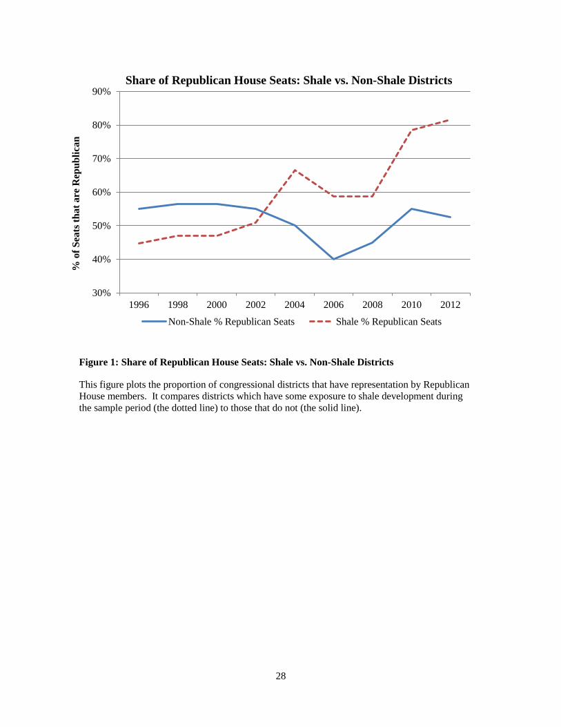
Figure 1: Share of Republican House Seats: Shale vs. Non-Shale Districts

This figure plots the proportion of congressional districts that have representation by Republican House members. It compares districts which have some exposure to shale development during the sample period (the dotted line) to those that do not (the solid line).

30%

40%

50%

60%

70%

80%

90%

1996 1998 2000 2002 2004 2006 2008 2010 2012

% o

f Sea

ts th

at a

re R

epub

lican

Share of Republican House Seats: Shale vs. Non-Shale Districts

Non-Shale % Republican Seats Shale % Republican Seats

28

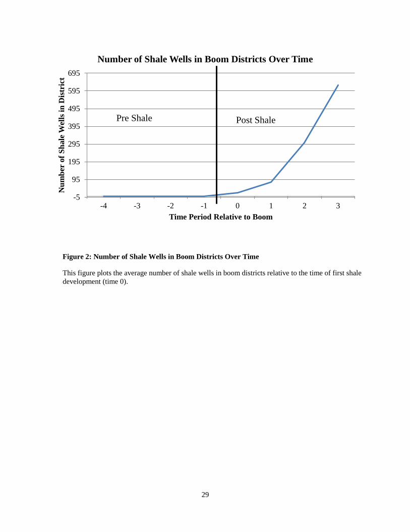
Figure 2: Number of Shale Wells in Boom Districts Over Time

This figure plots the average number of shale wells in boom districts relative to the time of first shale development (time 0).

-5

95

195

295

395

495

595

695

-4 -3 -2 -1 0 1 2 3

Num

ber

of S

hale

Wel

ls in

Dis

tric

t

Time Period Relative to Boom

Number of Shale Wells in Boom Districts Over Time

Pre Shale Post Shale

29

Figure 3: Effect of Boom on Republican Vote Share (House Districts)

This figure plots the relative percentage of votes received by republican house district candidates over time, based on when shale development first occurs in a district. Time 0 is the first election cycle that any shale development occurs in a district. The solid line represents the point estimates of Republican vote share relative to the initial period, while the dotted lines represent the 95% confidence interval.

-10

-5

0

5

10

15

20

-4 -3 -2 -1 0 1 2 3

% o

f Rep

ublic

an V

ote

Shar

e R

elat

ive

to

Aver

age

Effect of Boom on Republican Vote Share (House Districts)

30

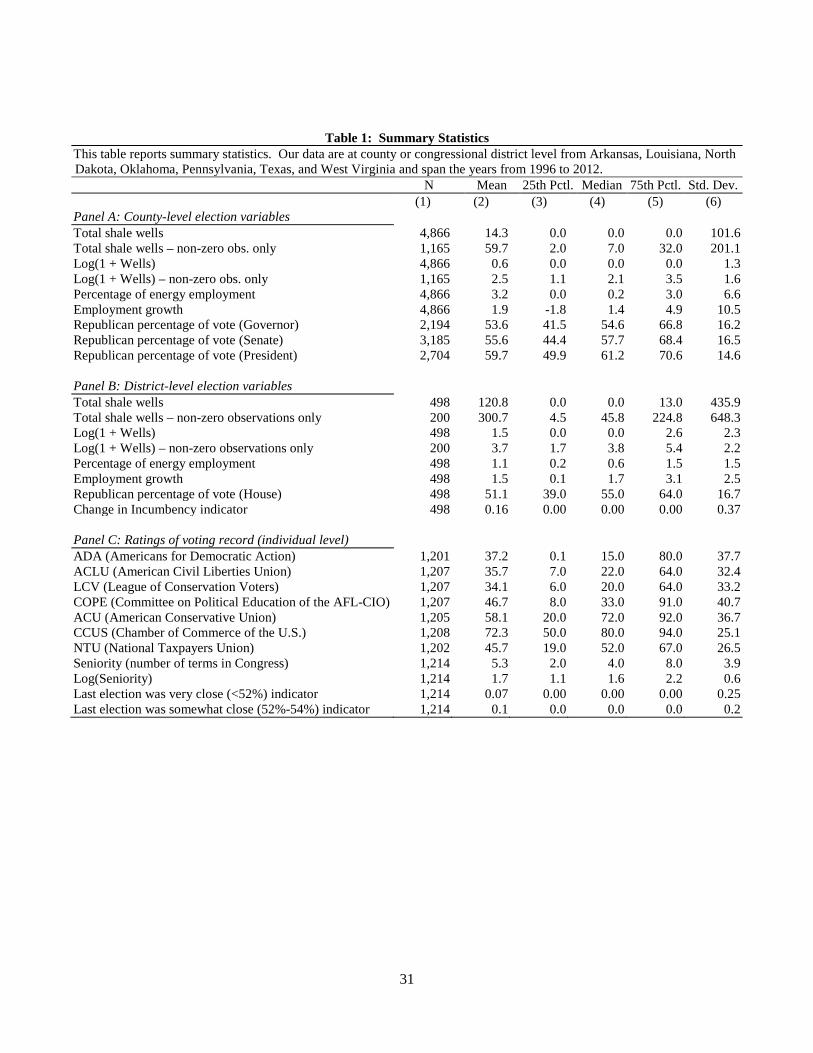
Table 1: Summary Statistics This table reports summary statistics. Our data are at county or congressional district level from Arkansas, Louisiana, North Dakota, Oklahoma, Pennsylvania, Texas, and West Virginia and span the years from 1996 to 2012.

N Mean 25th Pctl. Median 75th Pctl. Std. Dev. (1) (2) (3) (4) (5) (6)

Panel A: County-level election variables Total shale wells 4,866 14.3 0.0 0.0 0.0 101.6 Total shale wells – non-zero obs. only 1,165 59.7 2.0 7.0 32.0 201.1 Log(1 + Wells) 4,866 0.6 0.0 0.0 0.0 1.3 Log(1 + Wells) – non-zero obs. only 1,165 2.5 1.1 2.1 3.5 1.6 Percentage of energy employment 4,866 3.2 0.0 0.2 3.0 6.6 Employment growth 4,866 1.9 -1.8 1.4 4.9 10.5 Republican percentage of vote (Governor) 2,194 53.6 41.5 54.6 66.8 16.2 Republican percentage of vote (Senate) 3,185 55.6 44.4 57.7 68.4 16.5 Republican percentage of vote (President) 2,704 59.7 49.9 61.2 70.6 14.6

Panel B: District-level election variables Total shale wells 498 120.8 0.0 0.0 13.0 435.9 Total shale wells – non-zero observations only 200 300.7 4.5 45.8 224.8 648.3 Log(1 + Wells) 498 1.5 0.0 0.0 2.6 2.3 Log(1 + Wells) – non-zero observations only 200 3.7 1.7 3.8 5.4 2.2 Percentage of energy employment 498 1.1 0.2 0.6 1.5 1.5 Employment growth 498 1.5 0.1 1.7 3.1 2.5 Republican percentage of vote (House) 498 51.1 39.0 55.0 64.0 16.7 Change in Incumbency indicator 498 0.16 0.00 0.00 0.00 0.37

Panel C: Ratings of voting record (individual level) ADA (Americans for Democratic Action) 1,201 37.2 0.1 15.0 80.0 37.7 ACLU (American Civil Liberties Union) 1,207 35.7 7.0 22.0 64.0 32.4 LCV (League of Conservation Voters) 1,207 34.1 6.0 20.0 64.0 33.2 COPE (Committee on Political Education of the AFL-CIO) 1,207 46.7 8.0 33.0 91.0 40.7 ACU (American Conservative Union) 1,205 58.1 20.0 72.0 92.0 36.7 CCUS (Chamber of Commerce of the U.S.) 1,208 72.3 50.0 80.0 94.0 25.1 NTU (National Taxpayers Union) 1,202 45.7 19.0 52.0 67.0 26.5 Seniority (number of terms in Congress) 1,214 5.3 2.0 4.0 8.0 3.9 Log(Seniority) 1,214 1.7 1.1 1.6 2.2 0.6 Last election was very close (<52%) indicator 1,214 0.07 0.00 0.00 0.00 0.25 Last election was somewhat close (52%-54%) indicator 1,214 0.1 0.0 0.0 0.0 0.2

31

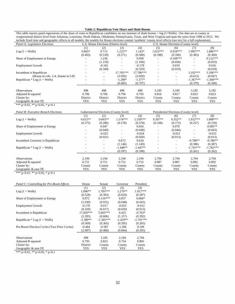
Table 2: Republican Vote Share and Shale Booms This table reports panel regressions of the share of votes to Republican candidates on our measure of shale booms = log (1+Wells). Our data are at county or congressional district level from Arkansas, Louisiana, North Dakota, Oklahoma, Pennsylvania, Texas, and West Virginia and span the years from 1996 to 2012. We include fixed time and geographic effects in all models; the models for House elections contain 'synthetic' county-level effects (see text for a full explanation). Panel A: Legislative Elections U.S. House Elections (District level) U.S. Senate Elections (County level) (1) (2) (3) (4) (5) (6) (7) (8) Log (1 + Wells) 0.865* 0.713 1.222** 1.143* 1.023*** 0.918*** 1.995*** 1.886*** (0.493) (0.539) (0.571) (0.580) (0.188) (0.180) (0.383) (0.369) Share of Employment in Energy - 1.236 - 0.958 - 0.108*** - 0.112*** - (1.218) - (1.184) - (0.036) - (0.035) Employment Growth - -0.165 - -0.178 - 0.019 - 0.016 - (0.349) - (0.329) - (0.019) - (0.018) Incumbent is Republican - - 17.765*** 17.786*** - - 5.102*** 5.106***

(House in cols. 1-4, Senate in 5-8) - - (3.926) (3.920) - - (0.613) (0.607) Republican * Log (1 + Wells) - - -1.289* -1.377* - - -1.367*** -1.360*** - - (0.685) (0.707) - - (0.379) (0.368) Observations 498 498 498 498 3,185 3,185 3,185 3,185 Adjusted R-squared 0.706 0.706 0.794 0.793 0.816 0.817 0.823 0.823 Cluster by: District District District District County County County County Geographic & year FE YES YES YES YES YES YES YES YES *** p<0.01, ** p<0.05, * p<0.1

Panel B: Executive Branch Elections Gubernatorial Elections (County level) Presidential Elections (County level) (1) (2) (3) (4) (5) (6) (7) (8) Log (1 + Wells) 0.615** 0.603** 1.574*** 1.558*** 0.397** 0.352** 1.912*** 1.888*** (0.275) (0.280) (0.578) (0.578) (0.168) (0.172) (0.257) (0.259) Share of Employment in Energy - 0.047 - 0.054 - 0.070 - 0.085** - (0.049) - (0.048) - (0.044) - (0.043) Employment Growth - -0.025 - -0.024 - -0.013 - -0.012 - (0.021) - (0.020) - (0.013) - (0.013) Incumbent Governor is Republican - - 0.673 0.634 - - -0.788** -0.780** - - (1.146) (1.149) - - (0.386) (0.387) Republican * Log (1 + Wells) - - -1.448** -1.447** - - -1.741*** -1.782***

- - (0.597) (0.598) - - (0.261) (0.262)

Observations 2,194 2,194 2,194 2,194 2,704 2,704 2,704 2,704 Adjusted R-squared 0.751 0.751 0.753 0.753 0.887 0.887 0.892 0.892 Cluster by: County County County County County County County County Geographic & year FE YES YES YES YES YES YES YES YES *** p<0.01, ** p<0.05, * p<0.1

Panel C: Controlling for Pre-Boom Effects House Senate Governor President (1) (2) (3) (4) Log (1 + Wells) 1.096** 1.783*** 1.270** 1.917*** (0.528) (0.393) (0.629) (0.287) Share of Employment in Energy 0.972 0.116*** 0.057 0.084* (1.030) (0.035) (0.048) (0.043) Employment Growth -0.179 0.017 -0.023 -0.012 (0.329) (0.017) (0.020) (0.013) Incumbent is Republican 17.820*** 5.065*** 0.425 -0.763* (2.295) (0.606) (1.157) (0.392) Republican * Log (1 + Wells) -1.380** -1.365*** -1.419** -1.791***

(0.569) (0.365) (0.595) (0.265) Pre-Boom Election Cycles (Two Prior Cycles) -0.464 -0.587 -1.206 0.109

(2.087) (0.468) (0.844) (0.305)

Observations 498 3,185 2,194 2,704 Adjusted R-squared 0.793 0.823 0.754 0.892 Cluster by: District County County County Geographic & year FE YES YES YES YES *** p<0.01, ** p<0.05, * p<0.1

32

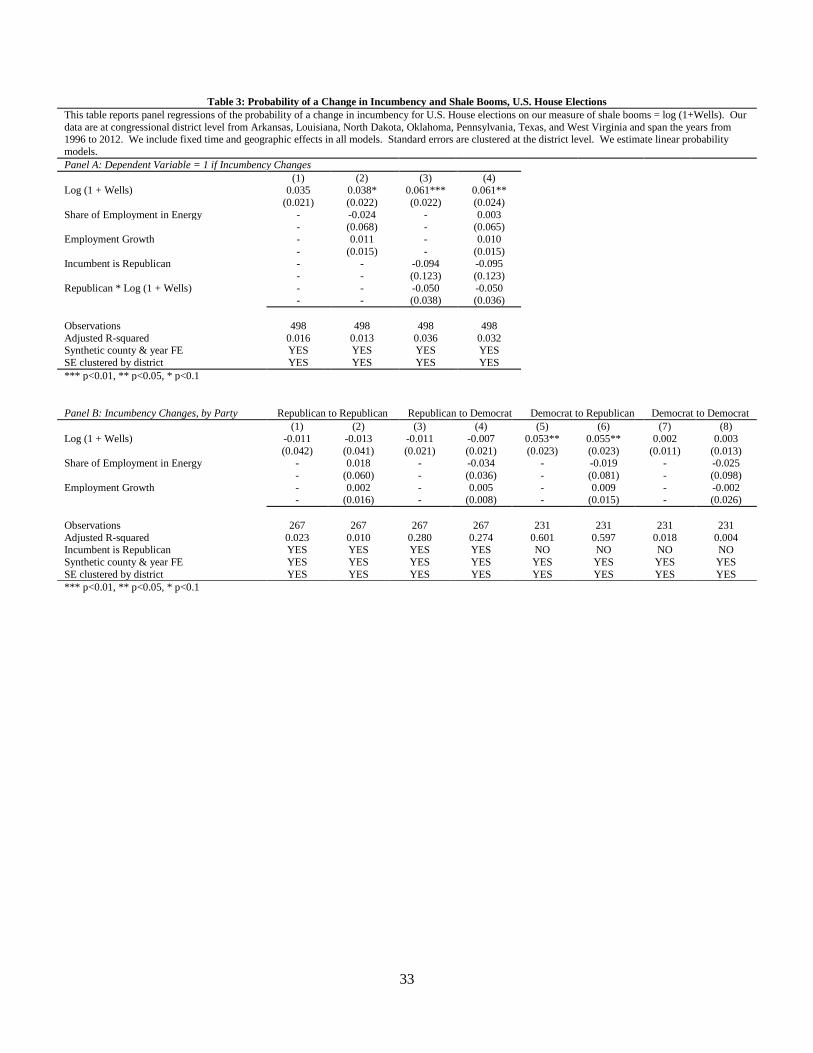
Table 3: Probability of a Change in Incumbency and Shale Booms, U.S. House Elections This table reports panel regressions of the probability of a change in incumbency for U.S. House elections on our measure of shale booms = log (1+Wells). Our data are at congressional district level from Arkansas, Louisiana, North Dakota, Oklahoma, Pennsylvania, Texas, and West Virginia and span the years from 1996 to 2012. We include fixed time and geographic effects in all models. Standard errors are clustered at the district level. We estimate linear probability models. Panel A: Dependent Variable = 1 if Incumbency Changes (1) (2) (3) (4) Log (1 + Wells) 0.035 0.038* 0.061*** 0.061** (0.021) (0.022) (0.022) (0.024) Share of Employment in Energy - -0.024 - 0.003 - (0.068) - (0.065) Employment Growth - 0.011 - 0.010 - (0.015) - (0.015) Incumbent is Republican - - -0.094 -0.095 - - (0.123) (0.123) Republican * Log (1 + Wells) - - -0.050 -0.050 - - (0.038) (0.036) Observations 498 498 498 498 Adjusted R-squared 0.016 0.013 0.036 0.032 Synthetic county & year FE YES YES YES YES SE clustered by district YES YES YES YES *** p<0.01, ** p<0.05, * p<0.1

Panel B: Incumbency Changes, by Party Republican to Republican Republican to Democrat Democrat to Republican Democrat to Democrat (1) (2) (3) (4) (5) (6) (7) (8) Log (1 + Wells) -0.011 -0.013 -0.011 -0.007 0.053** 0.055** 0.002 0.003 (0.042) (0.041) (0.021) (0.021) (0.023) (0.023) (0.011) (0.013) Share of Employment in Energy - 0.018 - -0.034 - -0.019 - -0.025 - (0.060) - (0.036) - (0.081) - (0.098) Employment Growth - 0.002 - 0.005 - 0.009 - -0.002 - (0.016) - (0.008) - (0.015) - (0.026) Observations 267 267 267 267 231 231 231 231 Adjusted R-squared 0.023 0.010 0.280 0.274 0.601 0.597 0.018 0.004 Incumbent is Republican YES YES YES YES NO NO NO NO Synthetic county & year FE YES YES YES YES YES YES YES YES SE clustered by district YES YES YES YES YES YES YES YES *** p<0.01, ** p<0.05, * p<0.1

33

Table 4A: ADA Roll-Call Voting Score and Shale Booms, U.S. House Members This table reports panel regressions of the ADA (Americans for Democratic Action) scores based on roll-call votes of U.S. House members on our measure of shale booms = log (1+Wells). The scores range from 0 to 100, with 100 meaning most liberal. Data are measured at the individual Congress member level from Arkansas, Louisiana, North Dakota, Oklahoma, Pennsylvania, Texas, and West Virginia, spanning the years from 1996 to 2012. We include fixed time and geographic effects in all models. Standard errors are clustered at the district level.

Without Congress Member Fixed Effects With Congress Member Fixed Effects

(1) (2) (3) (4) (5) (6) (7) (8)

Log (1 + Wells) -2.641*** -2.629*** 0.427 0.248 -1.429 -1.318 -7.401*** -7.193***

(0.798) (0.840) (0.684) (0.652) (1.461) (1.500) (2.386) (2.383)

Share of Employment in Energy - -0.082 - 1.770 - 1.283 - 0.841

- (2.069) - (1.351) - (1.382) - (1.276)

Employment Growth - -0.040 - 0.093 - 0.109 - 0.151

- (0.238) - (0.219) - (0.218) - (0.214)

Seniority - - - - -0.097 -0.008 - -

- - - - (0.608) (0.568) - -

Seniority * Log (1 + Wells) - - - - 0.237 0.206 - -

- - - - (0.199) (0.208) - -

Log of Seniority - - - - - - 6.153 6.345

- - - - - - (4.036) (4.083)

Log of Seniority * Log (1 + Wells) - - - - - - 3.657*** 3.520***

- - - - - - (1.197) (1.201)

Observations 1,201 1,201 1,201 1,201 1,201 1,201 1,201 1,201 Adjusted R-squared 0.712 0.711 0.906 0.906 0.906 0.906 0.908 0.908 Synthetic county & year FE YES YES YES YES YES YES YES YES SE clustered by district YES YES YES YES YES YES YES YES *** p<0.01, ** p<0.05, * p<0.1

34

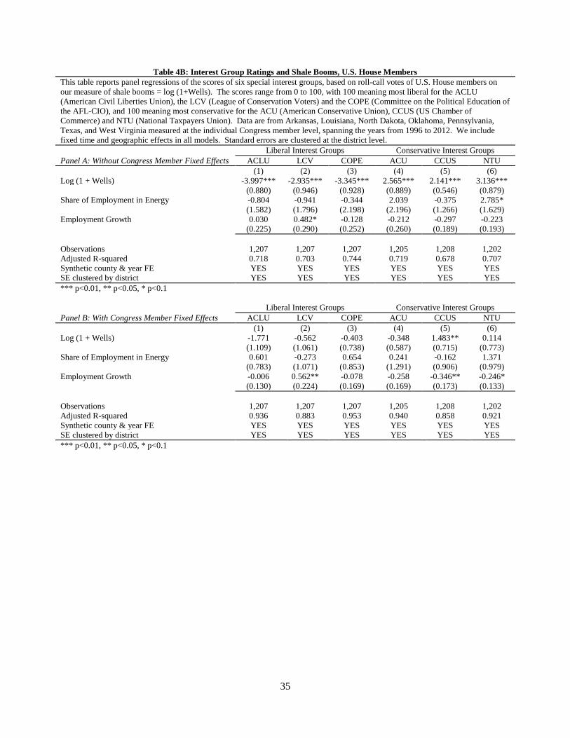
Table 4B: Interest Group Ratings and Shale Booms, U.S. House Members This table reports panel regressions of the scores of six special interest groups, based on roll-call votes of U.S. House members on our measure of shale booms = log (1+Wells). The scores range from 0 to 100, with 100 meaning most liberal for the ACLU (American Civil Liberties Union), the LCV (League of Conservation Voters) and the COPE (Committee on the Political Education of the AFL-CIO), and 100 meaning most conservative for the ACU (American Conservative Union), CCUS (US Chamber of Commerce) and NTU (National Taxpayers Union). Data are from Arkansas, Louisiana, North Dakota, Oklahoma, Pennsylvania, Texas, and West Virginia measured at the individual Congress member level, spanning the years from 1996 to 2012. We include fixed time and geographic effects in all models. Standard errors are clustered at the district level. Liberal Interest Groups Conservative Interest Groups Panel A: Without Congress Member Fixed Effects ACLU LCV COPE ACU CCUS NTU (1) (2) (3) (4) (5) (6) Log (1 + Wells) -3.997*** -2.935*** -3.345*** 2.565*** 2.141*** 3.136*** (0.880) (0.946) (0.928) (0.889) (0.546) (0.879) Share of Employment in Energy -0.804 -0.941 -0.344 2.039 -0.375 2.785* (1.582) (1.796) (2.198) (2.196) (1.266) (1.629) Employment Growth 0.030 0.482* -0.128 -0.212 -0.297 -0.223 (0.225) (0.290) (0.252) (0.260) (0.189) (0.193) Observations 1,207 1,207 1,207 1,205 1,208 1,202 Adjusted R-squared 0.718 0.703 0.744 0.719 0.678 0.707 Synthetic county & year FE YES YES YES YES YES YES SE clustered by district YES YES YES YES YES YES *** p<0.01, ** p<0.05, * p<0.1

Liberal Interest Groups Conservative Interest Groups

Panel B: With Congress Member Fixed Effects ACLU LCV COPE ACU CCUS NTU (1) (2) (3) (4) (5) (6) Log (1 + Wells) -1.771 -0.562 -0.403 -0.348 1.483** 0.114 (1.109) (1.061) (0.738) (0.587) (0.715) (0.773) Share of Employment in Energy 0.601 -0.273 0.654 0.241 -0.162 1.371 (0.783) (1.071) (0.853) (1.291) (0.906) (0.979) Employment Growth -0.006 0.562** -0.078 -0.258 -0.346** -0.246* (0.130) (0.224) (0.169) (0.169) (0.173) (0.133) Observations 1,207 1,207 1,207 1,205 1,208 1,202 Adjusted R-squared 0.936 0.883 0.953 0.940 0.858 0.921 Synthetic county & year FE YES YES YES YES YES YES SE clustered by district YES YES YES YES YES YES *** p<0.01, ** p<0.05, * p<0.1

35

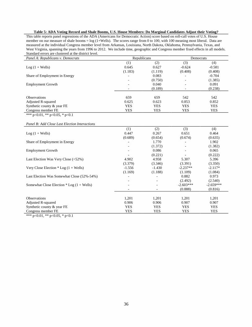
Table 5: ADA Voting Record and Shale Booms, U.S. House Members: Do Marginal Candidates Adjust their Voting? This table reports panel regressions of the ADA (Americans for Democratic Action) score based on roll-call votes of U.S. House member on our measure of shale booms = log (1+Wells). The scores range from 0 to 100, with 100 meaning most liberal. Data are measured at the individual Congress member level from Arkansas, Louisiana, North Dakota, Oklahoma, Pennsylvania, Texas, and West Virginia, spanning the years from 1996 to 2012. We include time, geographic and Congress member fixed effects in all models. Standard errors are clustered at the district level. Panel A: Republicans v. Democrats Republicans Democrats

(1) (2) (3) (4) Log (1 + Wells) 0.645 0.627 -0.624 -0.581 (1.183) (1.119) (0.408) (0.408) Share of Employment in Energy - 0.083 - -0.704 - (0.750) - (1.385) Employment Growth - 0.040 - 0.091 - (0.189) - (0.238) Observations 659 659 542 542 Adjusted R-squared 0.625 0.623 0.853 0.852 Synthetic county & year FE YES YES YES YES Congress member FE YES YES YES YES *** p<0.01, ** p<0.05, * p<0.1

Panel B: Add Close Last Election Interactions

(1) (2) (3) (4) Log (1 + Wells) 0.447 0.267 0.651 0.464 (0.689) (0.654) (0.674) (0.635) Share of Employment in Energy - 1.770 - 1.902 - (1.372) - (1.382) Employment Growth - 0.086 - 0.065

- (0.221) - (0.222) Last Election Was Very Close (<52%) 4.902 4.958 5.307 5.396 (3.379) (3.346) (3.391) (3.350) Very Close Election * Log (1 + Wells) -1.556 -1.430 -2.237** -2.117* (1.169) (1.188) (1.109) (1.084) Last Election Was Somewhat Close (52%-54%) - - 0.882 0.973 - - (2.492) (2.540) Somewhat Close Election * Log (1 + Wells) - - -2.603*** -2.659***

- - (0.888) (0.816)

Observations 1,201 1,201 1,201 1,201 Adjusted R-squared 0.906 0.906 0.907 0.907 Synthetic county & year FE YES YES YES YES Congress member FE YES YES YES YES *** p<0.01, ** p<0.05, * p<0.1

36