AMathematicallyDerivedNumberofResamplings forNoisyOptimization

Jialin Liu, David L. Saint-Pierre, Olivier Teytaudliu@lri.fr,davidls@lri.fr,teytaud@lri.fr

Team TAO, INRIA Saclay-CNRS-LRI, Univ. Paris-Sud, France

Noisy Black-box OptimizationObjective function f : Rd → ROptimum x∗ = argmin

x∈Rd

f(x)

Recommendation at iteration n xnRecommendation after #eval x#eval

Resampling rulesFor a sphere function,

√dσn ∼ O(||x − x∗||)

and σNoise ∼ O(1/√rn). To keep the standard

deviation of same order as the differences be-tween fitness values, which is dσn2, we shouldhave rn ∼ σn

−4d−2. Using a log-linear conver-gence log(σn) ' −Cn, we suggest C decreasingas Θ(1/d) in

rn ∼ exp(Cn)/d2. (1)

We use

Notation rnlinear n

quadratic n2

cubic n3

2exp 2n

exp/10 dexp( n10 )e

math1 dexp( 4n5d )/d2e

math2 dexp( n10 )/d2e

math3 dexp( n√d)/d2e

Conclusion• 2exp performs badly in large dimension;

• Polynomial rules perform badly in smalldimension;

• math2 has the best of both worlds andperforms nearly optimally among our non-adaptive rules in the considered setting,i.e. σNoise ∼ O(f).

Notationsf : fitness functiond: search space dimensionx: search point ∈ Rd

ω: random processn: generation indexrn: resampling number at generation n#eval: total number of evaluationsσn: step-size at generation nN : standard Gaussian random variable

Some References[1] Sandra Astete-Morales, Jialin Liu, and Olivier Tey-

taud. log-log convergence for noisy optimization. InProceedings of EA 2013, LLNCS. Springer, 2013.

[2] Anne Auger. Convergence results for the (1, λ)-sa-es using the theory of φ-irreducible markov chains.Theoretical Computer Science, 334(1):35–69, 2005.

[3] Olivier Teytaud, Jérémie Decock, et al. Noisy opti-mization complexity. In FOGA-Foundations of Ge-netic Algorithms XII-2013, 2013.

[4] Hervé Fournier and Olivier Teytaud. Lower boundsfor comparison based evolution strategies usingvc-dimension and sign patterns. Algorithmica,59(3):387–408, 2011.

Abstract• Resampling = classical tool for adapting evolution strategies (ES) to noisy optimization.

• Goal of this work: a conclusive answer for parameter-free resampling rules in simple settings.

• We work with Self-Adaptive (µ/µ,λ)-ES.

• Here, local noisy optimization (no local minima involved).

Convergence RateNoise-free case: log-linear convergence[2]

log ||xn||n

∼ A′ < 0 (2)

Noisy case: [1] proves that using exponential rules with ad hoc parameters can lead to this log-logconvergence.[3]

log ||x#eval||log(#eval)

∼ A′′ < 0 (3)

Simple Regret (SR) and slope(SR):

SR = Ef(x#eval)− Ef(x∗) (4)

slope(SR) = lim sup#eval

log (SR)

log(#eval)(5)

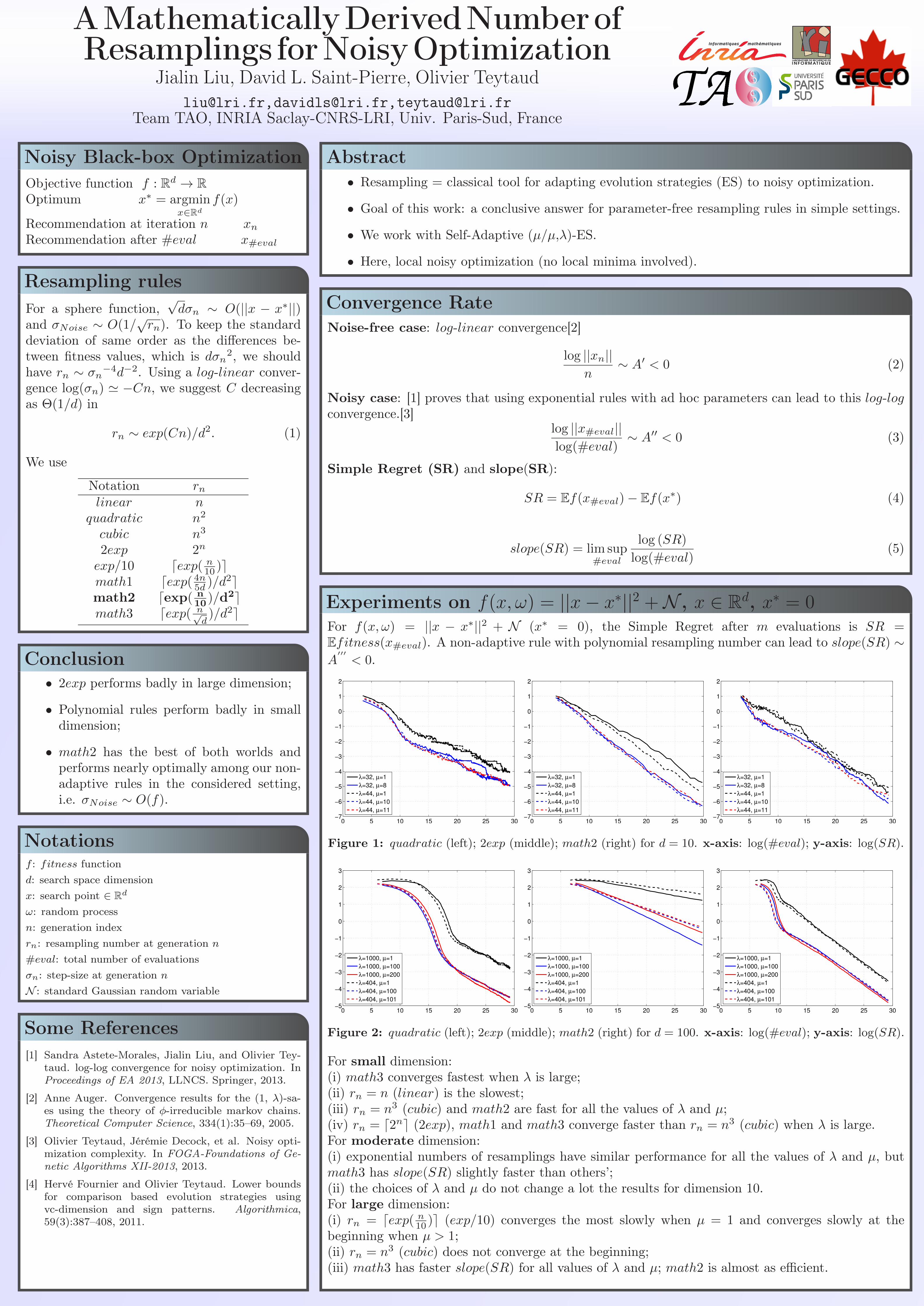
Experiments on f(x, ω) = ||x− x∗||2 +N , x ∈ Rd, x∗ = 0For f(x, ω) = ||x − x∗||2 + N (x∗ = 0), the Simple Regret after m evaluations is SR =Efitness(x#eval). A non-adaptive rule with polynomial resampling number can lead to slope(SR) ∼A

′′′< 0.

0 5 10 15 20 25 30−7

−6

−5

−4

−3

−2

−1

0

1

2

λ=32, µ=1

λ=32, µ=8

λ=44, µ=1

λ=44, µ=10

λ=44, µ=11

0 5 10 15 20 25 30−7

−6

−5

−4

−3

−2

−1

0

1

2

λ=32, µ=1

λ=32, µ=8

λ=44, µ=1

λ=44, µ=10

λ=44, µ=11

0 5 10 15 20 25 30−7

−6

−5

−4

−3

−2

−1

0

1

2

λ=32, µ=1

λ=32, µ=8

λ=44, µ=1

λ=44, µ=10

λ=44, µ=11

Figure 1: quadratic (left); 2exp (middle); math2 (right) for d = 10. x-axis: log(#eval); y-axis: log(SR).

0 5 10 15 20 25 30−5

−4

−3

−2

−1

0

1

2

3

λ=1000, µ=1

λ=1000, µ=100

λ=1000, µ=200

λ=404, µ=1

λ=404, µ=100

λ=404, µ=101

0 5 10 15 20 25 30−5

−4

−3

−2

−1

0

1

2

3

λ=1000, µ=1

λ=1000, µ=100

λ=1000, µ=200

λ=404, µ=1

λ=404, µ=100

λ=404, µ=101

0 5 10 15 20 25 30−5

−4

−3

−2

−1

0

1

2

3

λ=1000, µ=1

λ=1000, µ=100

λ=1000, µ=200

λ=404, µ=1

λ=404, µ=100

λ=404, µ=101

Figure 2: quadratic (left); 2exp (middle); math2 (right) for d = 100. x-axis: log(#eval); y-axis: log(SR).

For small dimension:(i) math3 converges fastest when λ is large;(ii) rn = n (linear) is the slowest;(iii) rn = n3 (cubic) and math2 are fast for all the values of λ and µ;(iv) rn = d2ne (2exp), math1 and math3 converge faster than rn = n3 (cubic) when λ is large.For moderate dimension:(i) exponential numbers of resamplings have similar performance for all the values of λ and µ, butmath3 has slope(SR) slightly faster than others’;(ii) the choices of λ and µ do not change a lot the results for dimension 10.For large dimension:(i) rn = dexp( n

10 )e (exp/10) converges the most slowly when µ = 1 and converges slowly at thebeginning when µ > 1;(ii) rn = n3 (cubic) does not converge at the beginning;(iii) math3 has faster slope(SR) for all values of λ and µ; math2 is almost as efficient.