Embed Size (px)
Citation preview

MigBSP:A New Approach for Processes Rescheduling
Management on Bulk Synchronous Parallel Applications
Candidate: Rodrigo da Rosa [email protected]
Advisor: Prof. Dr. Philippe Olivier Alexandre NavauxSandwich Advisor: Prof. Dr. Hans-Ulrich Heiβ
Thesis Defense - October, 2009 - Porto Alegre - Brazil
1 / 85

Outline
1 IntroductionContextMotivationRelated WorkOpportunities and ChallengesObjectiveHypothesis
2 Model of Processes Rescheduling
3 Evaluation Methodology
4 Model Evaluation
5 Final Considerations
2 / 85

Introduction: Context
Intensive applications still need more and more resourcesResources in network to compose a Grid infrastructure
Application models and programming interfaces to turn Grid usage a realityApplications in phases with points of synchronism
BSP (Bulk Synchronous Parallel) programming modelApplications (sorting, all sums, broadcast, data mining, computation fluid dynamics,molecular dynamics, minimum spanning tree, dense matrix multiplication)Composition of superstepsProgramming facilities and idea of execution costBSP processes can be mapped arbitrarily
BSP Processes
Global Communications
Local
Computations
Barrier Synchronization
3 / 85

Introduction: Motivation
1 ContextHow can we improve performance on BSP applications?Processes location management, since the synchronization barrier always wait forthe slowest processLoad balancing on processes management
2 Motivation: Approaches to offer load balancing on processes scheduling
Processes Scheduling
Programmer can adjust the processes-resources mapping by hand
Close coupling between the application and the load balancing mechanism
Other set of resources and/or another application requires a new effort for processes scheduling
Automatic load-balancing when BSP application is launched
Indicated mapping may become not effective during application execution
Dynamic behavior (both processes and infrastrucutre levels) can influence application execution
4 / 85

Introduction: Alternative
3 Alternative: BSP Processes Rescheduling
When to launch processes migration?Which processes are candidates formigration?Where to put an elected process amongthe candidates?How is the influence of migration costs ontransferring viability?How can we analyze the dynamicity issuein order to take better decisions onprocesses rescheduling treatment?
SourceResource
DestinationResource
TimeMigrationcosts
Processes Rescheduling
5 / 85

Introduction: Related Work
4 Some existing solutions: Analysis of the features
Hierarchical and cooperative scheduling LI:LAN:2005, YEUNG:2006, JACOBSEN:2007
Use of multiple metrics to compute the loadBHANDARKAR:2003, VOZMEDIANO:2005, DU:2007, HEISS:SCHIMITZ:1995
Use of multiple clusters and local networksKRIVOKAPIC:2000, YAGOUBI:2007, ZHANG:2009
Performance prediction KRIVOKAPIC:2000, YOUNG:2003, DONGARRA:2005
Migrations directives inside the application BHANDARKAR:2003
Use of fixed parameters for migration costs DONGARRA:2005 , processes
rescheduling interval UTRERA:2005, HERNANDEZ:2007 and application workload
SPOONDER:2003, KARP:2006
BSP model is attractive for dynamic and heterogeneous environments SONG:2006
Load balancing in BSP applications BONORDEN:2005, BONORDEN:2007
6 / 85

Introduction: Related Work
4 Some existing solutions: Analysis of the features
Hierarchical and cooperative scheduling LI:LAN:2005, YEUNG:2006, JACOBSEN:2007
Use of multiple metrics to compute the loadBHANDARKAR:2003, VOZMEDIANO:2005, DU:2007, HEISS:SCHIMITZ:1995
Use of multiple clusters and local networksKRIVOKAPIC:2000, YAGOUBI:2007, ZHANG:2009
Performance prediction KRIVOKAPIC:2000, YOUNG:2003, DONGARRA:2005
Migrations directives inside the application BHANDARKAR:2003
Use of fixed parameters for migration costs DONGARRA:2005 , processes
rescheduling interval UTRERA:2005, HERNANDEZ:2007 and application workload
SPOONDER:2003, KARP:2006
BSP model is attractive for dynamic and heterogeneous environments SONG:2006
Load balancing in BSP applications BONORDEN:2005, BONORDEN:2007
7 / 85

Introduction: Related Work
4 Some existing solutions: Analysis of the features
Hierarchical and cooperative scheduling LI:LAN:2005, YEUNG:2006, JACOBSEN:2007
Use of multiple metrics to compute the loadBHANDARKAR:2003, VOZMEDIANO:2005, DU:2007, HEISS:SCHIMITZ:1995
Use of multiple clusters and local networksKRIVOKAPIC:2000, YAGOUBI:2007, ZHANG:2009
Performance prediction KRIVOKAPIC:2000, YOUNG:2003, DONGARRA:2005
Migrations directives inside the application BHANDARKAR:2003
Use of fixed parameters for migration costs DONGARRA:2005 , processes
rescheduling interval UTRERA:2005, HERNANDEZ:2007 and application workload
SPOONDER:2003, KARP:2006
BSP model is attractive for dynamic and heterogeneous environments SONG:2006
Load balancing in BSP applications BONORDEN:2005, BONORDEN:2007
8 / 85

Introduction: Related Work
4 Some existing solutions: Analysis of the features
Hierarchical and cooperative scheduling LI:LAN:2005, YEUNG:2006, JACOBSEN:2007
Use of multiple metrics to compute the loadBHANDARKAR:2003, VOZMEDIANO:2005, DU:2007, HEISS:SCHIMITZ:1995
Use of multiple clusters and local networksKRIVOKAPIC:2000, YAGOUBI:2007, ZHANG:2009
Performance prediction KRIVOKAPIC:2000, YOUNG:2003, DONGARRA:2005
Migrations directives inside the application BHANDARKAR:2003
Use of fixed parameters for migration costs DONGARRA:2005 , processes
rescheduling interval UTRERA:2005, HERNANDEZ:2007 and application workload
SPOONDER:2003, KARP:2006
BSP model is attractive for dynamic and heterogeneous environments SONG:2006
Load balancing in BSP applications BONORDEN:2005, BONORDEN:2007
9 / 85

Introduction: Related Work
4 Some existing solutions: Analysis of the features
Hierarchical and cooperative scheduling LI:LAN:2005, YEUNG:2006, JACOBSEN:2007
Use of multiple metrics to compute the loadBHANDARKAR:2003, VOZMEDIANO:2005, DU:2007, HEISS:SCHIMITZ:1995
Use of multiple clusters and local networksKRIVOKAPIC:2000, YAGOUBI:2007, ZHANG:2009
Performance prediction KRIVOKAPIC:2000, YOUNG:2003, DONGARRA:2005
Migrations directives inside the application BHANDARKAR:2003
Use of fixed parameters for migration costs DONGARRA:2005 , processes
rescheduling interval UTRERA:2005, HERNANDEZ:2007 and application workload
SPOONDER:2003, KARP:2006
BSP model is attractive for dynamic and heterogeneous environments SONG:2006
Load balancing in BSP applications BONORDEN:2005, BONORDEN:2007
10 / 85

Introduction: Related Work
4 Some existing solutions: Analysis of the features
Hierarchical and cooperative scheduling LI:LAN:2005, YEUNG:2006, JACOBSEN:2007
Use of multiple metrics to compute the loadBHANDARKAR:2003, VOZMEDIANO:2005, DU:2007, HEISS:SCHIMITZ:1995
Use of multiple clusters and local networksKRIVOKAPIC:2000, YAGOUBI:2007, ZHANG:2009
Performance prediction KRIVOKAPIC:2000, YOUNG:2003, DONGARRA:2005
Migrations directives inside the application BHANDARKAR:2003
Use of fixed parameters for migration costs DONGARRA:2005 , processes
rescheduling interval UTRERA:2005, HERNANDEZ:2007 and application workload
SPOONDER:2003, KARP:2006
BSP model is attractive for dynamic and heterogeneous environments SONG:2006
Load balancing in BSP applications BONORDEN:2005, BONORDEN:2007
11 / 85

Introduction: Related Work
4 Some existing solutions: Analysis of the features
Hierarchical and cooperative scheduling LI:LAN:2005, YEUNG:2006, JACOBSEN:2007
Use of multiple metrics to compute the loadBHANDARKAR:2003, VOZMEDIANO:2005, DU:2007, HEISS:SCHIMITZ:1995
Use of multiple clusters and local networksKRIVOKAPIC:2000, YAGOUBI:2007, ZHANG:2009
Performance prediction KRIVOKAPIC:2000, YOUNG:2003, DONGARRA:2005
Migrations directives inside the application BHANDARKAR:2003
Use of fixed parameters for migration costs DONGARRA:2005 , processes
rescheduling interval UTRERA:2005, HERNANDEZ:2007 and application workload
SPOONDER:2003, KARP:2006
BSP model is attractive for dynamic and heterogeneous environments SONG:2006
Load balancing in BSP applications BONORDEN:2005, BONORDEN:2007
12 / 85

Introduction: Related Work
4 Some existing solutions: Analysis of the features
Hierarchical and cooperative scheduling LI:LAN:2005, YEUNG:2006, JACOBSEN:2007
Use of multiple metrics to compute the loadBHANDARKAR:2003, VOZMEDIANO:2005, DU:2007, HEISS:SCHIMITZ:1995
Use of multiple clusters and local networksKRIVOKAPIC:2000, YAGOUBI:2007, ZHANG:2009
Performance prediction KRIVOKAPIC:2000, YOUNG:2003, DONGARRA:2005
Migrations directives inside the application BHANDARKAR:2003
Use of fixed parameters for migration costs DONGARRA:2005 , processes
rescheduling interval UTRERA:2005, HERNANDEZ:2007 and application workload
SPOONDER:2003, KARP:2006
BSP model is attractive for dynamic and heterogeneous environments SONG:2006
Load balancing in BSP applications BONORDEN:2005, BONORDEN:2007
13 / 85

Introduction: Opportunities and Challenges
5 Opportunities of Work and Challenges
Analysis of processes stability consideringtheir computation and communication phases
Combination of multiple metrics in order tocontrol load rebalancing in BSP applications
Verification of the migration viability of eachcandidate process
Use of hierarchy to reduce the schedulingoverhead
Self-organizing in BSP processesrescheduling
14 / 85

Introduction: Objectives
6 ObjectiveKeywords: time, performance, BSP, load balancing, processes reschedulingModel for BSP processes reschedulingWithout changing the application code (middleware level)
BSP ProcessesBSP Processes
Before processes rescheduling
After processes rescheduling
Problem Statement: Given a BSP application and a set of processors on which BSP processes may be executed, our main objective is to control processes-processors remapping in order to reduce the supersteps' times
15 / 85

Introduction: Hypothesis
7 Hypothesis
How can we improve application’s performance?Our hypothesis is based on the following suppositions
Approximation of processes that establish a high degreeof communication can improve application’s performance
Migration of slow processes to faster processors canimprove performance
Avoid unproductive migrations can prevent possible lossof performance
Observation of the dynamicity issue can collaborate totake better decisions for performance improvement
Is our hypothesis true or false?
16 / 85

Outline
1 Introduction
2 Model of Processes ReschedulingDesign DecisionsScheduling ClassificationParallel Machine OrganizationDecision about the Moment for MigrationsDecision about Which Processes May MigrateDecision about Where to Put Migratable Processes
3 Evaluation Methodology
4 Model Evaluation
5 Final Considerations
17 / 85

Model: Design Decisions
MigBSP: Dynamic rescheduling model of BSP processes
BSP applications
MigBSP answers the following issues:
(i) “When” to launch the mechanism for processes migration(ii) “Which” processes are candidates for migration(iii) “Where” to put selected processes from the candidates ones
Main Issues on
Processes Migration
Controlling processes migration to different resources
Cover two from three possibilities to obtain better performance on BSPapplications SKILLICORN:1999
Computation balancingCommunication balancing
18 / 85

Model: Design Decisions
Without modifications in the application codeWithout prior knowledge about the applicationMiddleware levelEffortless way for attempting gains of performance
B Application
Programming Library + Rescheduling
Model
Implementation of the Rescheduling
Model
BSP Programming Library
Binary: BSP Application + Model
Execution in the Distributed System
together with Rescheduling Middleware
Compilation
and Linking
Submission
19 / 85

Model: Design Decisions
Dynamic scheduling
Avoid unproductive migrations
Use the notion of hierarchy
Grain of work: process
Main ideas
Observation of data that boostmigrations as well as informationsthat act in opposite direction
AdaptationsMinimization of model’s impact(overhead) on applicationexecution
Selection of good candidates formigration by analyzing thebehavior of each BSP process
20 / 85

Model: Design Decisions
Dynamic scheduling
Avoid unproductive migrations
Use the notion of hierarchy
Grain of work: process
Main ideas
Observation of data that boostmigrations as well as informationsthat act in opposite direction
AdaptationsMinimization of model’s impact(overhead) on applicationexecution
Selection of good candidates formigration by analyzing thebehavior of each BSP process
Processes
Migration Costs
21 / 85

Model: Design Decisions
Dynamic scheduling
Avoid unproductive migrations
Use the notion of hierarchy
Grain of work: process
Main ideas
Observation of data that boostmigrations as well as informationsthat act in opposite direction
AdaptationsMinimization of model’s impact(overhead) on applicationexecution
Selection of good candidates formigration by analyzing thebehavior of each BSP process
Processes'
state
BalancedUnbalanced
PostponedMore quickly
Rescheduling frequency
22 / 85

Model: Design Decisions
Dynamic scheduling
Avoid unproductive migrations
Use the notion of hierarchy
Grain of work: process
Main ideas
Observation of data that boostmigrations as well as informationsthat act in opposite direction
AdaptationsMinimization of model’s impact(overhead) on applicationexecution
Selection of good candidates formigration by analyzing thebehavior of each BSP process
Processes
23 / 85

Model: Scheduling Classification
MigBSP classification according to scheduling taxonomy from Casavant and KuhlCASAVANT:KUHL:1988
24 / 85

Model: Parallel Machine Organization
Communication Network
SMP Machine
Computer
LAN Network
Cluster
Node
ProcessorBSP process
Local networks, SMP machines e clusters
BSP processes can be viewed as virtual processors which are mapped to real(physical) processors
Asynchronous Communication: non-blocking sending and blocking receiving
25 / 85

Model: Parallel Machine Organization
Scheduling representation
Sk =
p0 p1 · · · pn−2 pn−1
P0 M0,0 M0,1 · · · M0,n−2 M0,n−1
P1 M1,0 M1,1 · · · M1,n−2 M1,n−1
......
......
...Pm−2 Mm−2,0 Mm−2,1 · · · Mm−2,n−2 Mm−2,n−1
Pm−1 Mm−1,0 Mm−1,1 · · · Mm−1,n−2 Mm−1,n−1
Sk means the mapping of processes(p) to processors P during the superstep k
Processors can receive more than one processes
Snapshot of the execution during a specific superstep
26 / 85

Model: Parallel Machine Organization
Set A
Set D
Set C
Set B
Set Manager
BSP Process -
Virtual Processor
Set E
Physical Processor
Scheduling message
Notion of Hierarchy: idea of Sets and Set Managers
Set Managers exchange scheduling data and act in order to choose a targetprocessor for migration
Scheduling code: linked to BSP processes and on each Set Manager
27 / 85

Model: Decision about the Moment for Migrations
Global Communication
Local
Computation
Barrier Synchronization
Processes Rescheduling
Barrier Synchronization
Collecting Information
for Processes MigrationSuperstep n
Superstep n+1
Answer the question “When”Use of an index called α which informs the interval for the next invocation ofprocesses reschedulingUse of two adaptations that act on rescheduling frequency
28 / 85

Model: Decision about the Moment for Migrations
First Adaptation: management of αThe Idea is to postpone the rescheduling call if the system is stable (processesare balanced) or turn it more frequent, otherwise.
time of the fastest process > average time . (1 - D)
time of the slowest process < average time . (1 + D)
�verage (A) of
the superstep
time of all processes
A . (1-D) A . (1+D)
execution time
BalancingUnbalancing Unbalancing
29 / 85

Model: Decision about the Moment for Migrations
First Adaptation: management of αThe Idea is to postpone the rescheduling call if the system is stable (processesare balanced) or turn it more frequent, otherwise.
time of the fastest process > average time . (1 - D)
time of the slowest process < average time . (1 + D)
Computation of the interval of supersteps for the next processes rescheduling
Do From superstep k to superstep k +α−1If Both Inequalities above are true
Increase α ’ by 1Else α ′ > α
Decrease α ’ by 1EndIf
EndDoCall for BSP processes reschedulingα = α ’
30 / 85

Model: Decision about the Moment for Migrations
Second Adaptation: management of D
The Idea is to delay the rescheduling call if a pattern without migrations in ω callsis observed
The larger the value of D, the higher the odds to increase α
Stability of the system according to D
γ ← Consecutive rescheduling calls without migrationsif γ ≥ ω
D← D + D2
Else if D > initial D and γ = 0D← D - D
2EndIf
31 / 85

Model: Decision about the Moment for Migrations
Processes Rescheduling
Processes Rescheduling
Superstep 1 Superstep alpha Superstep k Superstep k+alpha-1
Alpha' ComputationTime
Example of a BSP application execution with data from the model
Use of k , α e α ’
32 / 85

Model: Decision about Which Processes May Migrate
Answer the question “Which”
Employment of three metrics
(i) Computation
(ii) Communication
(iii) Memory
Idea:
To migrate a process with largeprocessing time, which presentshigh communication with otherprocess of a specific Set andpresents a low migration cost
Methodology:
Potential of Migration (PM) computation on each BSP process
PM(i, j) informs the viability to migrate process i to Set j
33 / 85

Model: Decision about Which Processes May Migrate
Computation Metric: CMP(i,j)
Computation Pattern - Indicates the stability, or regularity, of the process regardingthe amount of performed instructions at each superstepComputation time prediction (Aging concept)Performance degree of a Set
CMP(i, j) = Wcomp . Pcomp(i) . CTPk+α−1(i) . ISetk+α−1(j)
34 / 85
Model: Decision about Which Processes May Migrate
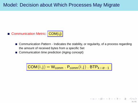
Communication Metric: COM(i,j)
Communication Pattern - Indicates the stability, or regularity, of a process regardingthe amount of received bytes from a specific SetCommunication time prediction (Aging concept)
COM(i, j) = Wcomm . Pcomm(i, j) . BTPk+α−1
35 / 85

Model: Decision about Which Processes May Migrate
Memory Metric: MEM(i,j)
Process’ memoryTime to transfer 1 byte between process i and Set jCosts related to migration operations (depending on both the operating system andthe used migration tool)
MEM(i, j) = Wmem . ( M(i) . T (i, j) + Mig(i, j) )
36 / 85

Model: Decision about Which Processes May Migrate
Potential of Migration: PM(i,j)
Analogy of Force from PhysicsMigration of process i to Set j
Computation Metric
BSP ProcessesMigration
Métrica Comunicação
Memory Metric
FavourOpposite
PM(i, j) = CMP(i, j)+COM(i, j)−MEM(i, j)
37 / 85

Model: Decision about Which Processes May Migrate
Idea of metrics’ weight: Change the actuation of a force
Set Managers exchange the highest PM(i, j) of each process
Two heuristics to choose the candidates for migration
(i) Processes with PM larger than Max(PM).x are candidates
(ii) Only the process with the highest PM is candidate
Main idea: MigBSP does not perform all processes-processors tests in the rescheduling moment
38 / 85

Model: Decision about Where to Put Migratable Processes
Answer to the question “Where”
Manager of the target Set selects a processor p based on BSP processesmapped to it, as well as on its theoretical capacity and load
Migration evaluation of process i : currently it executes on processor p′ and maymigrate to Set j that has the processor p
t1 = time(p) + bytes . Transfer(i,j) + migration costs
t2 = time(p’) + bytes . Transf(i,j)
Migration: t1 < t2
Process i can migrate to the same Set which it belongs currently
39 / 85

Outline
1 Introduction
2 Model of Processes Rescheduling
3 Evaluation MethodologyBasic DecisionsMigration CostsExecution ScenariosParallel Machine Organization
4 Model Evaluation
5 Final Considerations
40 / 85

Evaluation Methodology: Basic Decisions
Use of simulation GROEN:2009
Reproducibility of resultsOur focus is on the validation of MigBSP’s algorithmsEasier way for resource allocation (always available)
Simulator requirements - Criteria definition
Processes manipulation (creating and migrating)Message passing among the processesAsynchronous communication and barrier synchronizationPossibility to express the dynamism and heterogeneity
Analyzed simulators
MicroGridGridSimSimGridOptorSimNS2
41 / 85

Evaluation Methodology: Basic Decisions
SimGrid Simulator LEGRAND:CASANOVA:2003
XML files which describe both the application’s platform and deployment
Deterministic simulator
Special function for processes migration
Study of significant BSP applications
Lattice-Boltzmann - Computational Fluid Dynamics
Smith-Watermann - Sequence alignment based onDynamic Programming
LU Decomposition - Linear Equations
Regular
Irregular
Irregular
42 / 85

Evaluation Methodology: Basic Decisions
SimGrid Simulator LEGRAND:CASANOVA:2003
XML files which describe both the application’s platform and deployment
Deterministic simulator
Special function for processes migration
Study of significant BSP applications
Lattice-Boltzmann - Computational Fluid Dynamics
Smith-Watermann - Sequence alignment based onDynamic Programming
LU Decomposition - Linear Equations
Regular
Irregular
Irregular
43 / 85

Evaluation Methodology: Migration Costs
We need data to feed our model
Computation and Communication Metrics
Computation and Communication behaviors of each BSP processData from the nodes (load and theoretical capacity)Data from the network (available bandwidth)
How about migration costs (Memory Metric) ?
Tests with AMPI (Adaptive MPI)Preliminary tests were performed using a single cluster
Mapping of obtained migration costs to our Grid architecture
migration time grid = migration time cluster . bandwidth clusterbandwidth grid
Example: Considering 100Mbits/s and 0.2s as bandwidth and migration costs fora single cluster situation, the migration time on a multi-hop network when thebandwidth is 60Mbits/s will be 0.33s.
44 / 85

Evaluation Methodology: Execution Scenarios
Development of three execution scenarios
Scenarios Application execution MigBSP execution Enabling Migrations
Scenario i •Scenario ii • •Scenario iii • • •
Possible Comparisons
Scenarios i and ii - Model’s intrusiveness on application execution
Scenarios i and iii - Analyze the performance gain/loss with processes migrations
Scenarios ii and iii - Observe changes occurred on application execution takinginto account performed migrations
45 / 85
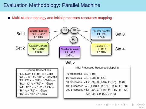
Evaluation Methodology: Parallel Machine
Multi-cluster topology and initial processes-resources mapping
R3
Cluster ICEI1...I1121.6 GHz
Cluster FrontalF1...F61 GHz
Cluster Corisco"C1...C16"1 GHz
Cluster AquarioA1...A202 GHz
R1 R2Cluster Labtec"L1 ... L20"1.5 GHz
"L1...L20" <-> "R1" = 1 Gbps"C1...C16" <-> "R1" = 100 Mbps
"F1...F6" <-> "R2" = 100 Mbps
"I1...I112" <-> "R2" = 1 Gbps
"A1...A20" <-> "R3" = 1 Gbps
"R1" <-> "R2" = 1 Gbps
"R2" <-> "R3" = 1 Gbps
Network Connections
Set 1
Set 2
Set 3
Set 4
Set 5
Initial Processes-Resources Mapping
200 processes = L {1-20}, C {1-16}, F {1-6}, I {1-112},
A {1-20}, L {1-20}, C {1-6}
25 processes = L {1-20}, C {1-5}
50 processes = L {1-20}, C {1-16}, F {1-6}, I {1-8}
100 processes = L {1-20}, C {1-16}, F {1-6}, I {1-58}
10 processes = L {1-10}
46 / 85

Outline
1 Introduction
2 Model of Processes Rescheduling
3 Evaluation Methodology
4 Model EvaluationLattice-Boltzmann ApplicationSmith-Watermann ApplicationLU Decomposition ApplicationResults Remarks
5 Final Considerations
47 / 85

Model Evaluation: Lattice Boltzmann
Lattice-Boltzmann ApplicationModeling
Regular applicationVertical domain decompositionProcess i passes data to its right-sided neighbor i +1Matrix requires the computation of 1010 instructions
Matrix partition will influence the workload of the processes
Amount of communication is independent of the partition scheme
p1 p2 pn p2np1 p2
(a) Decomposition among
n processes
(b) Decomposition among
2n processes
Parameters: α = 2, 4, 8 and 16. D = 0.5, ω = 3
Only the process with the highest PM is candidate for migration48 / 85

Model Evaluation: Lattice Boltzmann
Analyzing the gain with processes migration considering both scenarios i and iiiand 2000 supersteps
0
200
400
600
800
1000
1200
1400
Scenario i
Scenario iii with initial α = 4
Scenario iii with initial α = 8
Scenario iii with initial α = 16
10 processes 25 processes 50 processes 100 processes
Time in Seconds
200 processes
49 / 85

Model Evaluation: Lattice Boltzmann
Barrier times on two situations
Times captured when 2000 supersteps are crossed
Times captures in process p1
Processes Scenario i Scenario iii
10 0.005380s 0.005380s25 0.023943s 0.010765s50 0.033487s 0.025360s
100 0.036126s 0.028337s200 0.043247s 0.031440s
Conclusion: Processes reassignment can contribute for decreasing the time spent in barrier functions
50 / 85

Model Evaluation: Lattice Boltzmann
MigBSP overhead when executing Lattice Boltzmann method with α 4.Performance Function PF = time in scenario ii
time in scenario i
� !"# $ $"# % %"# &
%!!!'()*+,(-+*(
$!!!'()*+,(-+*(
#!!'()*+,(-+*(
$!!'()*+,(-+*(
#!'()*+,(-+*(
$!'()*+,(-+*(
.)/0-12/'3.
$"$45
$"$&6
$"5!7
$"$$&
$"%$8
$"776
$"!5#
$"$76
$"%48
$"!%%
$"!7&
$"!84
$"!$&
$"!%#
$"!#%
$"!!5
$"!$&
$"!%8
25
Processes
50
Processes
100
Processes
51 / 85

Model Evaluation: Smith-Watermann
p1 p2�� ��
s1
s2
s3
s4 s5 s6 s7
p1 p2 p3 p4
Computational load Supersteps and
communications
Smith-Watermann application - Dynamic Programming
Irregular application
The more intense the shading, the greater the computational load of the cell
Local sequence alignmentComputational density changes along the matrix’s cellsThe algorithms proceeds in series of wavefronts diagonally across the matrix
52 / 85

Model Evaluation: Smith-Watermann
p1 p2 p3 p4
s1
s2
s3
s4 s5 s6 s7
p1 p2 p3 p4
Computational load Supersteps and
communications
Initial scheduling: Column-based processes allocation
Square matrix with order n
2n−1 supersteps are crossed to compute the matrixEach process will be involved on n superstepsEach process p sends data to its neighbor p +1
Parameters: Percentage of processes are candidates (80% of the highest PMs);α = 2, 4 8 and 16; D = 0.5 and ω = 3
53 / 85

Model Evaluation: Smith-Watermann
Scenarios mat. 10×10 mat. 25×25 mat. 50×50 mat. 100×100 mat. 200×200
Scenario i 13.34s 40.74s 92.59s 162.66s 389.91s
Scen. ii
α = 2 14.15s 43.05s 95.70s 166.57s 394.68s
α = 4 14.71s 42.24s 94.84s 165.66s 393.75s
α = 8 13.78s 41.63s 94.03s 164.80s 392.85s
α = 16 13.42s 41.28s 93.36s 164.04s 392.01s
Scen. iii
α = 2 13.09s 35.97s 85.95s 150.57 374.62s
α = 4 11.94s 34.82s 84.65s 148.89s 375.53s
α = 8 13.82s 41.64s 83.00s 146.55s 374.38s
α = 16 12.40s 40.64s 85.21s 162.49s 374.40s
Application execution varying: matrix size, scenario and αSquare matrix with order n implies in 2n−1 supersteps
54 / 85

Model Evaluation: Smith-Watermann
Scenarios mat. 10×10 mat. 25×25 mat. 50×50 mat. 100×100 mat. 200×200
Scenario i 13.34s 40.74s 92.59s 162.66s 389.91s
Scen. ii
α = 2 14.15s 43.05s 95.70s 166.57s 394.68s
α = 4 14.71s 42.24s 94.84s 165.66s 393.75s
α = 8 13.78s 41.63s 94.03s 164.80s 392.85s
α = 16 13.42s 41.28s 93.36s 164.04s 392.01s
Scen. iii
α = 2 13.09s 35.97s 85.95s 150.57 374.62s
α = 4 11.94s 34.82s 84.65s 148.89s 375.53s
α = 8 13.82s 41.64s 83.00s 146.55s 374.38s
α = 16 12.40s 40.64s 85.21s 162.49s 374.40s
Comparison between scenarios i and ii
Low overhead≤ 5.6%
55 / 85

Model Evaluation: Smith-Watermann
Scenarios mat. 10×10 mat. 25×25 mat. 50×50 mat. 100×100 mat. 200×200
Scenario i 13.34s 40.74s 92.59s 162.66s 389.91s
Scen. ii
α = 2 14.15s 43.05s 95.70s 166.57s 394.68s
α = 4 14.71s 42.24s 94.84s 165.66s 393.75s
α = 8 13.78s 41.63s 94.03s 164.80s 392.85s
α = 16 13.42s 41.28s 93.36s 164.04s 392.01s
Scen. iii
α = 2 13.09s 35.97s 85.95s 150.57 374.62s
α = 4 11.94s 34.82s 84.65s 148.89s 375.53s
α = 8 13.82s 41.64s 83.00s 146.55s 374.38s
α = 16 12.40s 40.64s 85.21s 162.49s 374.40s
Comparison between scenarios i and iii
Maximum gain with migrations = 14.4 %
56 / 85

Model Evaluation: Smith-Watermann
0 10 20 30 40 50 60 99
0
2
4
6
8
10
α = 2
α = 4
α = 8
Number of Supersteps
Number of Migrations
. . .
Matrix 50x50
99 supersteps
System is stable and α always increase at each superstep
57 / 85

Model Evaluation: Smith-Watermann
0 10 20 30 40 50 60 99
0
2
4
6
8
10
α = 2
α = 4
α = 8
Number of Supersteps
Number of Migrations
. . .
p{37-42}
to Aquario
Rescheduling attemps
without migration
p{21-29} to Aquario
Scenario iii: α 2 = 85,95s, α 4 = 84,65s and α 8 = 83,00s
Scenario i: 92,59s
α 8 presents only one call without migration
58 / 85

Model Evaluation: Smith-Watermann
Graph of migrations with matrix 200x200
Observations
Before: L=40, C=22, F=6, I=112, A=20
After: L=34, C=2, I=112, A=52
Application: CPU-bound
Migrations from slower to faster clusters
Without knowledge of the application
Labtec Corisco
Frontal Ice
Aquario
Finishing
Starting
59 / 85

Model Evaluation: LU Decomposition
LU Decomposition
Decomposition: A = L . U
Usage
This method is used to solve linear equations easierIt is also employed for calculating the inverse of a matrix and its determinant
60 / 85

Model Evaluation: LU Decomposition
LU Decomposition
Decomposition: A = L . U
Usage
This method is used to solve linear equations easierIt is employed to calculate the inverse of a matrix and its determinant too
L
U
61 / 85

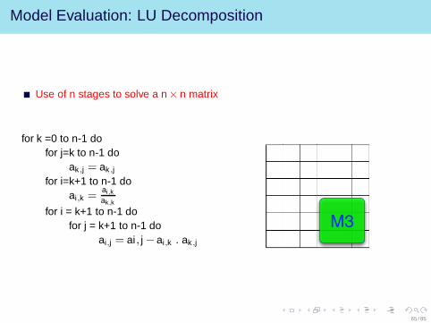
Model Evaluation: LU Decomposition
Use of n stages to solve a n×n matrix
for k =0 to n-1 dofor j=k to n-1 do
ak ,j = ak ,j
for i=k+1 to n-1 doai,k =
ai,kak,k
for i = k+1 to n-1 dofor j = k+1 to n-1 do
ai,j = ai, j−ai,k . ak ,j
M0
62 / 85

Model Evaluation: LU Decomposition
Use of n stages to solve a n×n matrix
for k =0 to n-1 dofor j=k to n-1 do
ak ,j = ak ,j
for i=k+1 to n-1 doai,k =
ai,kak,k
for i = k+1 to n-1 dofor j = k+1 to n-1 do
ai,j = ai, j−ai,k . ak ,j
M1
63 / 85

Model Evaluation: LU Decomposition
Use of n stages to solve a n×n matrix
for k =0 to n-1 dofor j=k to n-1 do
ak ,j = ak ,j
for i=k+1 to n-1 doai,k =
ai,kak,k
for i = k+1 to n-1 dofor j = k+1 to n-1 do
ai,j = ai, j−ai,k . ak ,j
M2
64 / 85
Model Evaluation: LU Decomposition
Use of n stages to solve a n×n matrix
for k =0 to n-1 dofor j=k to n-1 do
ak ,j = ak ,j
for i=k+1 to n-1 doai,k =
ai,kak,k
for i = k+1 to n-1 dofor j = k+1 to n-1 do
ai,j = ai, j−ai,k . ak ,j
M3
65 / 85
Model Evaluation: LU Decomposition
Use of n stages to solve a n×n matrix
for k =0 to n-1 dofor j=k to n-1 do
ak ,j = ak ,j
for i=k+1 to n-1 doai,k =
ai,kak,k
for i = k+1 to n-1 dofor j = k+1 to n-1 do
ai,j = ai, j−ai,k . ak ,jM4
66 / 85

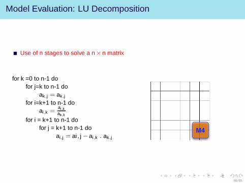
Model Evaluation: LU Decomposition
Use of n stages to solve a n×n matrix
for k =0 to n-1 dofor j=k to n-1 do
ak ,j = ak ,j
for i=k+1 to n-1 doai,k =
ai,kak,k
for i = k+1 to n-1 dofor j = k+1 to n-1 do
ai,j = ai, j−ai,k . ak ,jM5
67 / 85

Model Evaluation: LU Decomposition
Use of n stages to solve a n×n matrix
for k =0 to n-1 dofor j=k to n-1 do
ak ,j = ak ,j
for i=k+1 to n-1 doai,k =
ai,k
ak,k
for i = k+1 to n-1 dofor j = k+1 to n-1 do
ai,j = ai, j−ai,k . ak ,j
Cartesian distribution ofprocesses: SxP
Good utilization of processes ateach superstep
0 1 2 0 1 2
1
0
00 01 02 00 01 02
10 11 12 10 11 12
10 11 12 10 11 12
10 11 12 10 11 12
00 01 02 00 01 02
00 01 02 00 01 02
0
0
1
1
68 / 85

Model Evaluation: LU Decomposition
Use of n stages to solve a n×n matrix
for k =0 to n-1 dofor j=k to n-1 do
ak ,j = ak ,j
for i=k+1 to n-1 doai,k =
ai,k
ak,k
for i = k+1 to n-1 dofor j = k+1 to n-1 do
ai,j = ai, j−ai,k . ak ,j
Cartesian distribution ofprocesses: SxP
Good utilization of processes ateach superstep
00 01 02 00 01 02
0 1 2 0 1 2
1
0
00 01 02 00 01 02
10 11 12 10 11 12
10 11 12 10 11 12
10 11 12 10 11 12
00 01 02 00 01 02
0
0
1
1
69 / 85

Model Evaluation: LU Decomposition
Use of n stages to solve a n×n matrix
for k =0 to n-1 dofor j=k to n-1 do
ak ,j = ak ,j
for i=k+1 to n-1 doai,k =
ai,kak,k
for i = k+1 to n-1 dofor j = k+1 to n-1 do
ai,j = ai, j−ai,k . ak ,j
Cartesian distribution ofprocesses: SxP
Process ak ,j performs a multicastto the processes that belong to itssame column
00 01 02 00 01 02
0 1 2 0 1 2
1
0
00 01 02 00 01 02
10 11 12 10 11 12
10 11 12 10 11 12
10 11 12 10 11 12
00 01 02 00 01 02
0
0
1
1
70 / 85

Model Evaluation: LU Decomposition
Use of n stages to solve a n×n matrix
for k =0 to n-1 dofor j=k to n-1 do
ak ,j = ak ,j
for i=k+1 to n-1 doai,k =
ai,kak,k
for i = k+1 to n-1 dofor j = k+1 to n-1 do
ai,j = ai, j−ai,k . ak ,j
Cartesian distribution ofprocesses: SxP
Process ai,k performs a multicastto processes that belong to itssame line
00 01 02 00 01 02
0 1 2 0 1 2
1
0
00 01 02 00 01 02
10 11 12 10 11 12
10 11 12 10 11 12
10 11 12 10 11 12
00 01 02 00 01 02
0
0
1
1
71 / 85

Model Evaluation: LU Decomposition
Parameters: Percentage of processes are candidates (80% of the highest PMs);α = 2, 4 8 and 16; D = 0.5 and ω = 3Performance graph for 5000× 5000 matrix
400
600
800
1000
1200
1400Scenario i - LU application simply
Scenario ii - App. with MigBSP without migrations
Scenario iii - App. with MigBSP allowing migrations
Time in seconds
25processes
50processes
100processes
200processes
72 / 85

Model Evaluation: Results Remarks
Model’s overhead is lower than 8%
Avoiding unproductive migrations
Performance gains up to 19%
Performance gains without changing the application code
MigBSP does not work with prior knowledge about theapplication
73 / 85

Outline
1 Introduction
2 Model of Processes Rescheduling
3 Evaluation Methodology
4 Model Evaluation
5 Final ConsiderationsContributions and ResultsFuture WorksPublicationsAcknowledgments
74 / 85

Final Considerations: Contributions and Results
MigBSP solves the followingquestions about load balancingon processes level
Scientific Contributions
Hypothesis
Results Analysis
When to launch processesrescheduling
A sliding α that controls therescheduling frequency
Which processes arecandidates for migration
Analogy of force to describeprocesses migration
PM(i, j) = CMP(i, j)+COM(i, j)−MEM(i, j)
Where to put a selectedprocess
Consideration of migration costs
75 / 85

Final Considerations: Contributions and Results
MigBSP solves the followingquestions about load balancingon processes level
Scientific Contributions
Hypothesis
Results Analysis
MigBSP’s contributions on BSPprocesses rescheduling arethreefold
Combination of three metrics forcreating the Potential ofMigration (PM)
Adaptation on the reschedulingfrequency
Use of both Computation andCommunication Patterns
PhD Thesis
76 / 85

Final Considerations: Contributions and Results
MigBSP solves the followingquestions about load balancingon processes level
Scientific Contributions
Hypothesis
Results Analysis
Approximation of processes thatestablish a high degree ofcommunication can improveapplication’s performance
Migration of slow processes tofaster processors can improveperformance
Avoid unproductive migrations canprevent possible loss of performance
Observation of dynamicity issuecan collaborate to take better decisionsfor performance improvement
Is our hypothesis true or false? TRUE
77 / 85

Final Considerations: Contributions and Results
MigBSP solves the followingquestions about load balancingon processes level
Scientific Contributions
Hypothesis
Results Analysis
Performance gains up to 19%
User/programmer does not needto change her/his application
A large number of superstepscontribute to amortize theMigBSP’s overhead
The larger the size of theproblem, the higher the gain withprocesses migration
The key role of the MemoryMetric on PM calculus
78 / 85

Final Considerations: Future Work
Use of a new heuristic to choose the processes that will be migrated
Analysis of Computation and Communication patterns that act over a collection ofsupersteps instead of every superstep
Test MigBSP when changing the availability of the resources
Evaluate MigBSP with different migration costs techniques
79 / 85

Final Considerations: Publications
Publications during the period of the doctorate
Publications in local and regional conferences - WSPPD and ERAD
Next submissions
Journal of Communication and ComputerParallel Processing Letters
80 / 85

Final Considerations: Publications
81 / 85

Final Considerations
I
5 MIGBSP MODEL EVALUATION . . . . . . . . . . . . . . . . . . . . . . 97
5.1 Objectives . . . . . . . . . . . . . . . . . . . . . . . . . . . . . . . . . . . 97
5.2 Simulating MigBSP Model . . . . . . . . . . . . . . . . . . . . . . . . . . 98
5.2.1 Platform and Processes Deployment Definition . . . . . . . . . . . . . . 99
5.2.2 Writing BSP A pplication . . . . . . . . . . . . . . . . . . . . . . . . . . 101
5.2.3 M igBSP Development . . . . . . . . . . . . . . . . . . . . . . . . . . . . 101
5.3 Scientific Methodology . . . . . . . . . . . . . . . . . . . . . . . . . . . . 102
5.3.1 A nalyzing the M igration Costs . . . . . . . . . . . . . . . . . . . . . . . 102
5.3.2 Scenarios of Tests . . . . . . . . . . . . . . . . . . . . . . . . . . . . . . 103
5.3.3 Multi-C luster Testbed A rchitecture . . . . . . . . . . . . . . . . . . . . . 104
5.4 Lattice Boltzmann Method . . . . . . . . . . . . . . . . . . . . . . . . . 104
5.4.1 Modeling . . . . . . . . . . . . . . . . . . . . . . . . . . . . . . . . . . 104
5.4.2 Results . . . . . . . . . . . . . . . . . . . . . . . . . . . . . . . . . . . . 106
5.5 Smith-Watermann Application . . . . . . . . . . . . . . . . . . . . . . . 111
5.5.1 Modeling . . . . . . . . . . . . . . . . . . . . . . . . . . . . . . . . . . 111
5.5.2 Results . . . . . . . . . . . . . . . . . . . . . . . . . . . . . . . . . . . . 112
5.6 LU Decomposition Application . . . . . . . . . . . . . . . . . . . . . . . 117
5.6.1 Modeling . . . . . . . . . . . . . . . . . . . . . . . . . . . . . . . . . . 118
5.6.2 Results . . . . . . . . . . . . . . . . . . . . . . . . . . . . . . . . . . . . 120
5.7 Summary . . . . . . . . . . . . . . . . . . . . . . . . . . . . . . . . . . . 122
�������Under Evaluation
IPCCC 2009
82 / 85

Final Considerations: Acknowledgments
I would like to express my especial thanks toMy familyPhilippe Olivier Alexandre NavauxHans-Ulrich HeiβAlexandre da Silva CarissimiJorg SchneiderLaercio Lima PillaMembers of the juryGPPD group
Thanks to the following institutions
UFRGSTU-BerlinCAPESCNPqDAAD
83 / 85

MigBSP:A New Approach for Processes Rescheduling
Management on Bulk Synchronous Parallel Applications
Candidate: Rodrigo da Rosa [email protected]
Advisor: Prof. Dr. Philippe Olivier Alexandre NavauxSandwich Advisor: Prof. Dr. Hans-Ulrich Heiβ
Thesis Defense - October, 2009 - Porto Alegre - Brazil
84 / 85

Adaptations on Processes Rescheduling
(a) Scenario ii ( Rescheduling model + without migrations + both adaptations)
(b) Scenario iii (Rescheduling model + with migrations + both adaptations)
4 8 12 20 36 68
4 8 12 24 40 72
Legend
Rescheduling call with migration Rescheduling call where a migration is selected but not done
Rescheduling call where none migrations are done or selected
4 8 12 16 20 24 28 32 4036 44 48 52 56 60 64 100
(d) Scenario iii (Rescheduling model + with migrations + without adaptations)
16
85 / 85


![[curso, UFRGS],](https://img.pdfslide.net/doc/110x75/55cf98d7550346d03399f776/curso-ufrgs.jpg)