數值模擬與志願運算數值模擬與志願運算-- -- 輕鬆上手參加輕鬆上手參加 LHCLHC 實驗實驗

Yuan CHAO ( 趙元 )(National Taiwan University, Taipei, Taiwan)

COSCUP2016/08/20-21

我是誰？Yuan CHAO (John)

YChao...

研究員高能物理使用 OSS 做研究 ...

4

簡介簡介數值計算模擬數值計算模擬蒙地卡羅方法蒙地卡羅方法面積法計算面積法計算 ππ布豐投針問題布豐投針問題參與參與 LHCLHC 實驗實驗志願運算志願運算公開數據公開數據

數值計算與模擬

用 CPU 來描述真實的世界與做假想實驗

7

標準模型標準模型 Standard ModelStandard Model

~10-18 m宇宙的尺度 http://htwins.net/scale2/~10-1 m

膠子 光子 W/Z子 重力子

強作用力 電磁力 弱作用力 重力

夸克

輕子

奈米 =10-9 m

現今的處理器仍然無法處理原子分子O(1020 - 1030)

1PB = 1015 Byte

以巨觀統計的角度來看問題

統計 → 機率

碰撞 → 壓力

能量 → 溫度

蒙地卡羅法 ( 近似解 )拉斯維加斯法 ( 正解 )

蒙地卡羅法 ( 給定時間 )拉斯維加斯法 ( 未知時間 )

The first thoughts and attempts I made to practice [the Monte Carlo Method]were suggested by a question which occurred to me in 1946 as I was

convalescing from an illness and playing solitaires. The question was what arethe chances that a Canfield solitaire laid out with 52 cards will come outsuccessfully? After spending a lot of time trying to estimate them by pure

combinatorial calculations, I wondered whether a more practical method than"abstract thinking" might not be to lay it out say one hundred times and simply

observe and count the number of successful plays. This was already possible toenvisage with the beginning of the new era of fast computers, and I immediately

thought of problems of neutron diffusion and other questions of mathematicalphysics, and more generally how to change processes described by certain

differential equations into an equivalent form interpretable as a succession ofrandom operations. Later [in 1946], I described the idea to John von Neumann,

and we began to plan actual calculations.

–- Stanislaw Ulam

https://en.wikipedia.org/wiki/Monte_Carlo_method

蒙地卡羅法求 π

面積法

r

Pie are squared

r

Pie are square πr2

r

Pie are square πr2對稱r

Pie are square πr2對稱r

https://upload.wikimedia.org/wikipedia/commons/8/84/Pi_30K.gif

import randomimport numpyimport ROOT

m_total = 10**5m_radius = 1

def in_circle(point): x = point[0] y = point[1] return (x**2 + y**2) < m_radius**2

m_count = m_inside = 0

c1 = ROOT.TCanvas("pi", "#pi", 600, 600)m_x = numpy.linspace(0, 1.,101)m_y = (1.**2 - m_x**2)**0.5

c1.cd()

g = ROOT.TGraph(len(m_x), m_x, m_y)g.SetTitle("#pi")

g.GetXaxis().SetTitle("x")g.GetYaxis().SetTitle("y")

hist1 = ROOT.TH2F("hist1", "#pi outside", 100, 0, 1, 100, 0, 1)hist2 = ROOT.TH2F("hist2", "#pi inside", 100, 0, 1, 100, 0, 1)

for i in range(m_total): point = random.random()*m_radius, random.random()*m_radius if in_circle(point): hist2.Fill(point[0], point[1]) m_inside += 1 else: hist1.Fill(point[0], point[1]) m_count += 1

pi = (m_inside * 1.0 / m_count) * 4

print(pi)

hist1.SetMarkerColor(4)hist1.Draw("same")hist2.SetMarkerColor(2)hist2.Draw("same")

g.SetLineWidth(3)g.Draw("same")

c1.SaveAs("pi.png")

$ python pyroot_pi.py3.14108

git@github.com:yuanchao/MCnVC.git

布豐投針問題George Louis, Comte de Buffon in 18th

https://en.wikipedia.org/wiki/Georges-Louis_Leclerc,_Comte_de_Buffon

布豐投針問題對稱性

https://en.wikipedia.org/wiki/Buffon%27s_needle

al

b

t

布豐投針法求 πMario Lazzarini in 1901

https://en.wikipedia.org/wiki/Buffon%27s_needle

拋了3408次針，得到π的近似值為355/113。

布豐投針法求 π對稱性

考慮針的中心點 x 落在

的機率都相同，針的方向也是

與線條相交時的距離

所以相交的機率為

https://en.wikipedia.org/wiki/Buffon%27s_needle

al

b

t

http://blog.linux.org.tw/~jserv/archives/002004.html

數值模擬的軟體多半基於蒙地卡羅演算法ex. GEANT 模擬器

https://geant4.web.cern.ch/geant4/

越精確的結果→ 需要越多計算量 ( 時間 )

大型強子對撞型加速器也需要數值模擬

LHCLHC

WWWWWW的出生地的出生地 !!!!!!

SERN

志願運算？Volunteer computing

公民素人參與大實驗

現場有多少人參加過這個 FFT 分析的計算？

CMS 實驗組~3000 科學家

182 研究單位 來自 42 個國家~130 電算中心

200k – 250k jobs 同時執行使用 WLCG 運算網格

37

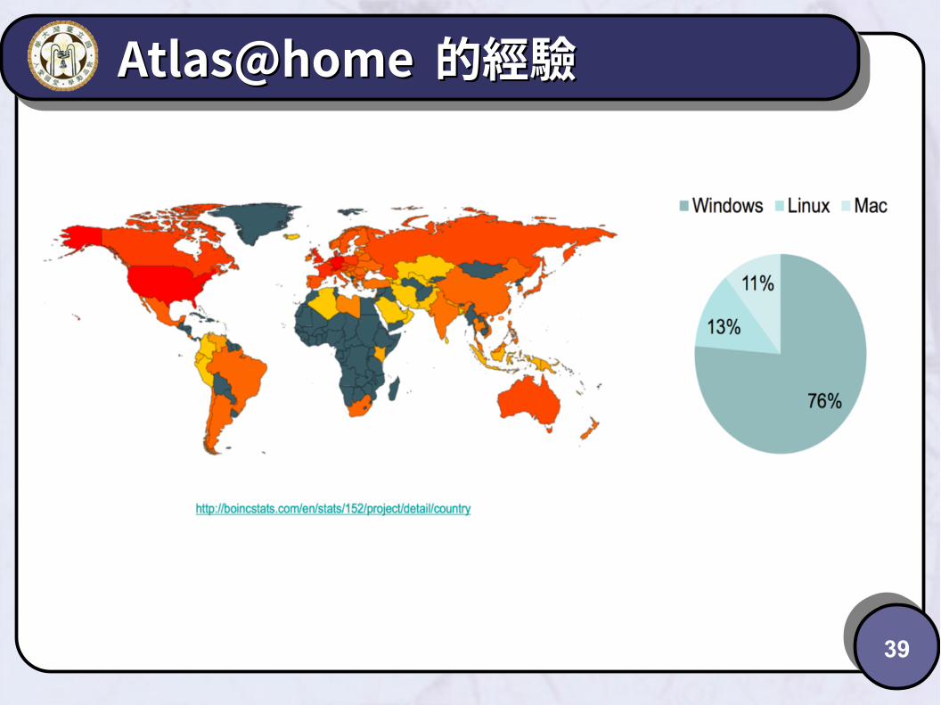
Atlas@home Atlas@home 的經驗的經驗也執行實際的模擬工作也執行實際的模擬工作

每個批次每個批次 2525 個事例 個事例 (( 正常為正常為 10001000 事例事例 ))執行時間執行時間 1 – 41 – 4 小時 小時 (( 正常為正常為 88 核心核心 1212 小時小時 ))虛擬環境映象檔虛擬環境映象檔 ~500 MB (~500 MB ( 展開約 展開約 1GB )1GB )下載數據下載數據 1 – 100 MB1 – 100 MB回傳數據回傳數據 ~100MB~100MB虛擬環境記憶體需求虛擬環境記憶體需求 2GB2GB

如何參與？如何參與？下載下載 BOINCBOINC 用戶端軟體用戶端軟體 (Mac, Linux, Windows)(Mac, Linux, Windows)選擇選擇 Atlas@homeAtlas@home 或或 CMS@homeCMS@home 並建立帳號並建立帳號開始計算！開始計算！BOINCBOINC 軟體可以排程，在閒置時執行軟體可以排程，在閒置時執行

http://boinc.berkeley.edu/

38

Atlas@home Atlas@home 的經驗的經驗

39

Atlas@home Atlas@home 的經驗的經驗

40

Atlas@home Atlas@home 的經驗的經驗

開放數據Open Data

CMS 今年又開放了新的實驗數據

http://opendata.cern.ch/https://home.cern/about/updates/2016/04/cms-releases-new-batch-lhc-open-data

總容量已經達到 300TB您的硬碟放得下嗎？ ;)

詳細使用請見 2013/4 年簡報

http://www.slideshare.net/yuanchao/ychao-20140720

http://www.slideshare.net/yuanchao/ychao-20130803

以上

謝謝