A combined approach for anomaly detection in production systemsusing machine learning techniques

Università degli Studi di TriesteDipartimento di Ingegneria e Architettura

Corso di Laurea Magistrale in Ingegneria Informatica

Laureando:David Fanjkutić

Relatore:prof. Eric Medvet

Correlatori:dott. Alexander Maierdott. Andreas Bunte

Anno accademico 2014/2015

Sessione straordinaria

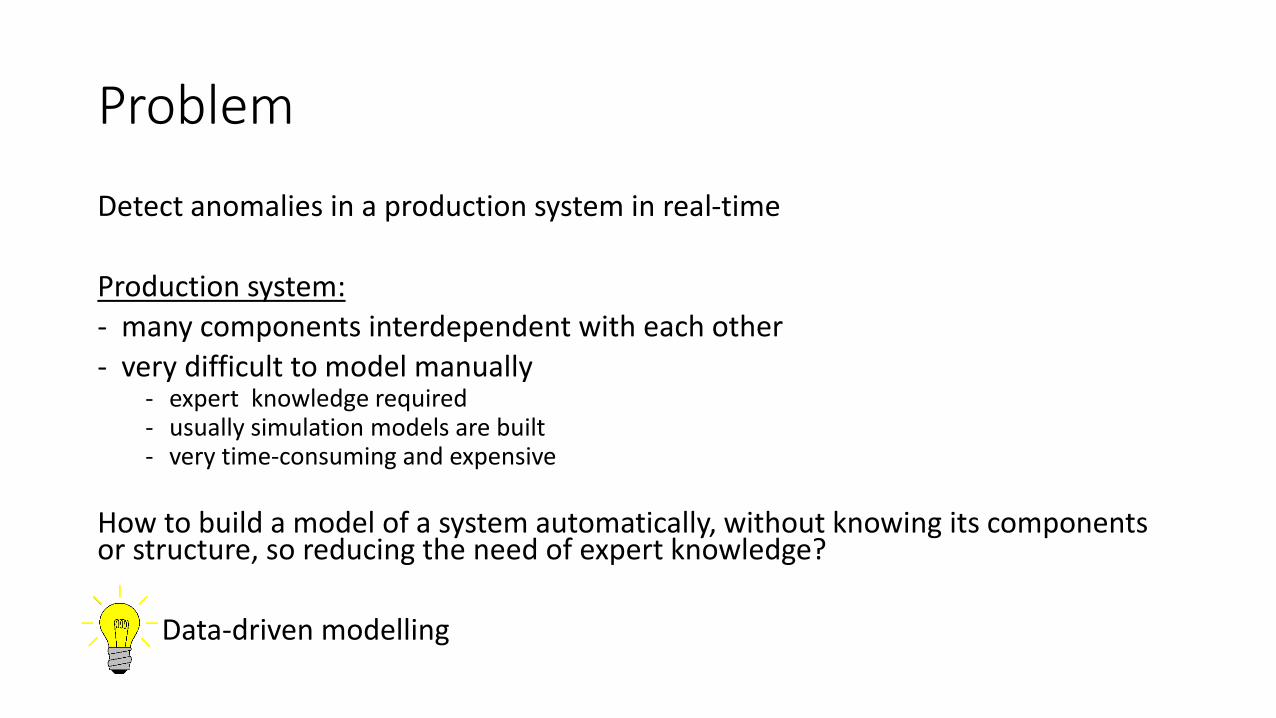
Problem

Detect anomalies in a production system in real-time

Production system:

- many components interdependent with each other

- very difficult to model manually- expert knowledge required- usually simulation models are built- very time-consuming and expensive

How to build a model of a system automatically, without knowing its components or structure, so reducing the need of expert knowledge?

Data-driven modelling

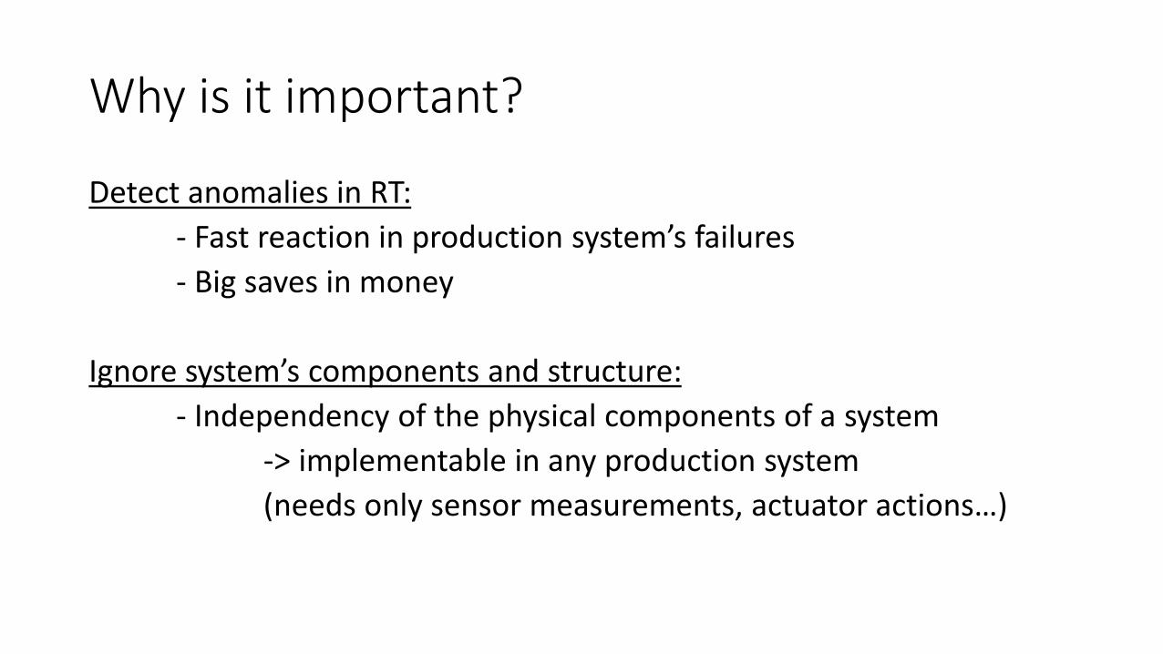
Why is it important?

Detect anomalies in RT:

- Fast reaction in production system’s failures

- Big saves in money

Ignore system’s components and structure:

- Independency of the physical components of a system

-> implementable in any production system

(needs only sensor measurements, actuator actions…)

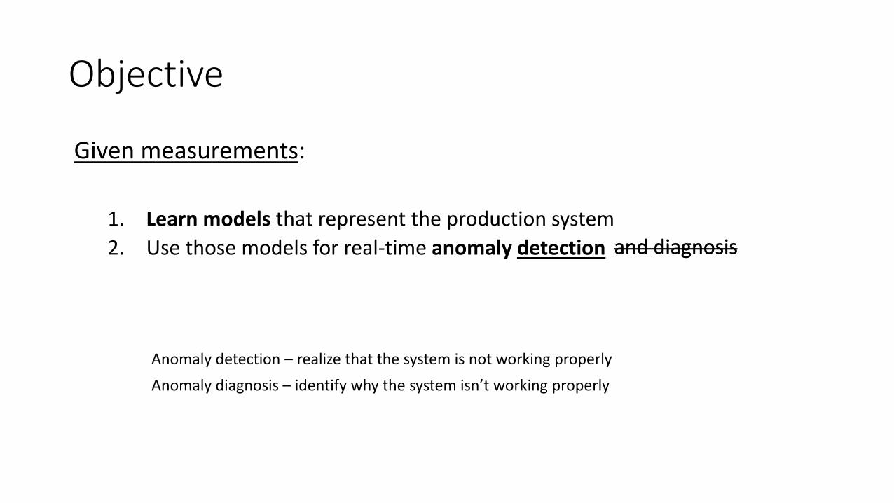
Objective

Given measurements:

1. Learn models that represent the production system

2. Use those models for real-time anomaly detection and diagnosisand diagnosis

Anomaly detection – realize that the system is not working properly

Anomaly diagnosis – identify why the system isn’t working properly

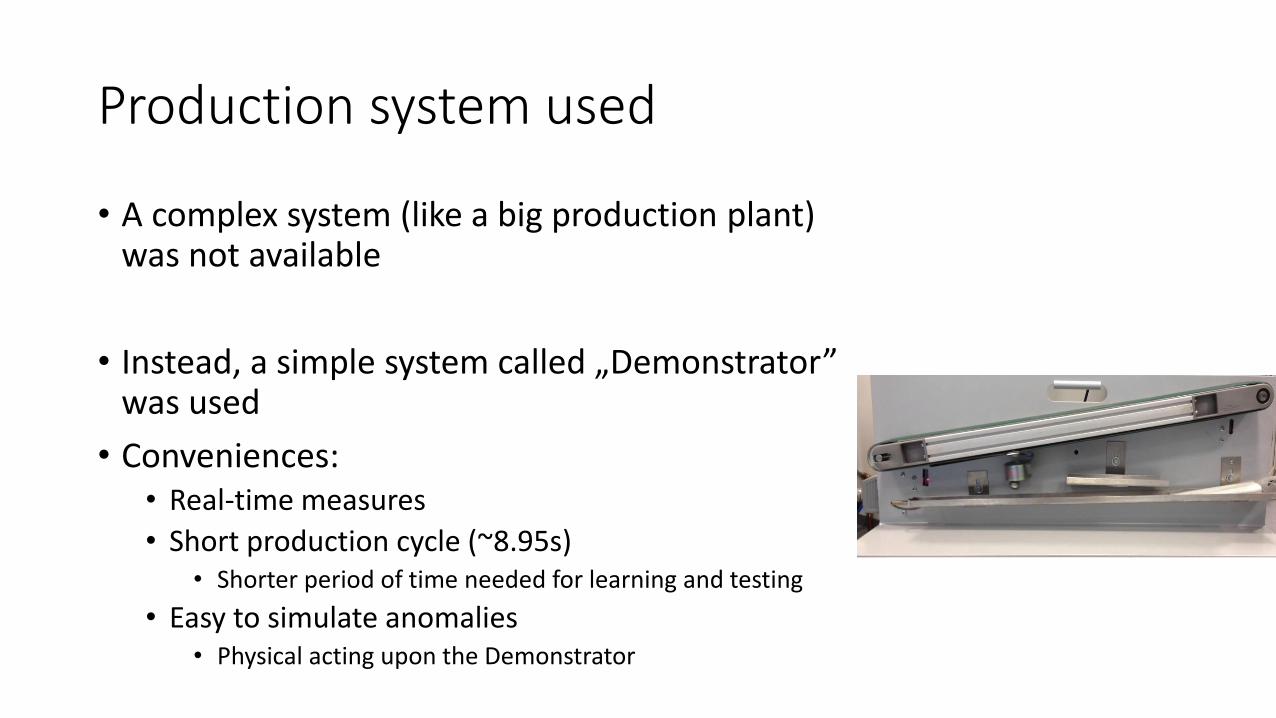
Production system used

• A complex system (like a big production plant) was not available

• Instead, a simple system called „Demonstrator” was used

• Conveniences:• Real-time measures

• Short production cycle (~8.95s)• Shorter period of time needed for learning and testing

• Easy to simulate anomalies• Physical acting upon the Demonstrator

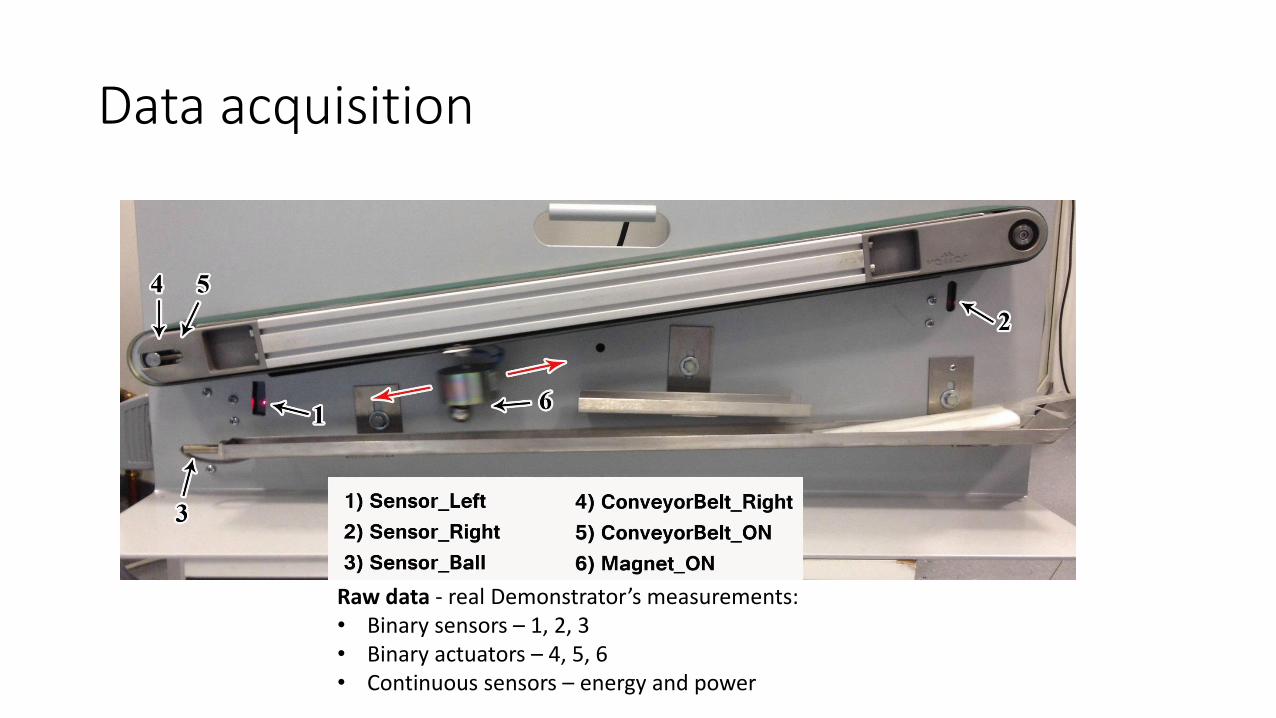
Data acquisition

Raw data - real Demonstrator’s measurements:• Binary sensors – 1, 2, 3• Binary actuators – 4, 5, 6• Continuous sensors – energy and power

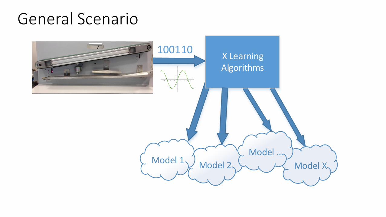
General Scenario

100110X LearningAlgorithms

Model XModel 2Model 1

Model …

Definitions

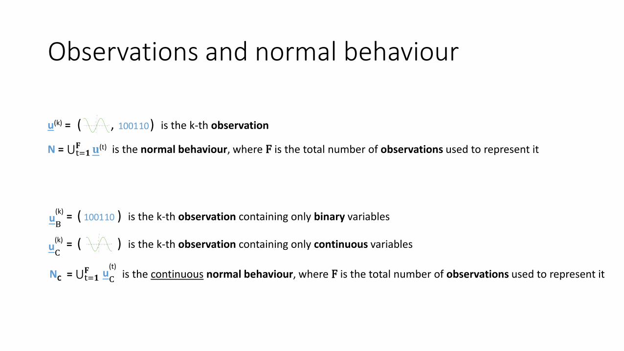
• OBSERVATION– a vector of system’s measurements at a point in time, contains discrete(binary) and continuous variables

• NORMAL BEHAVIOUR – an ordered set (by time) of observations that occurred while the system was functioning normally

• MODEL – an abstract representation of a system learned from normal behaviour

• ANOMALY – an observation which is not coherent with the learned models

What does „coherent with learned models” mean?? We’ll see in a few slides…

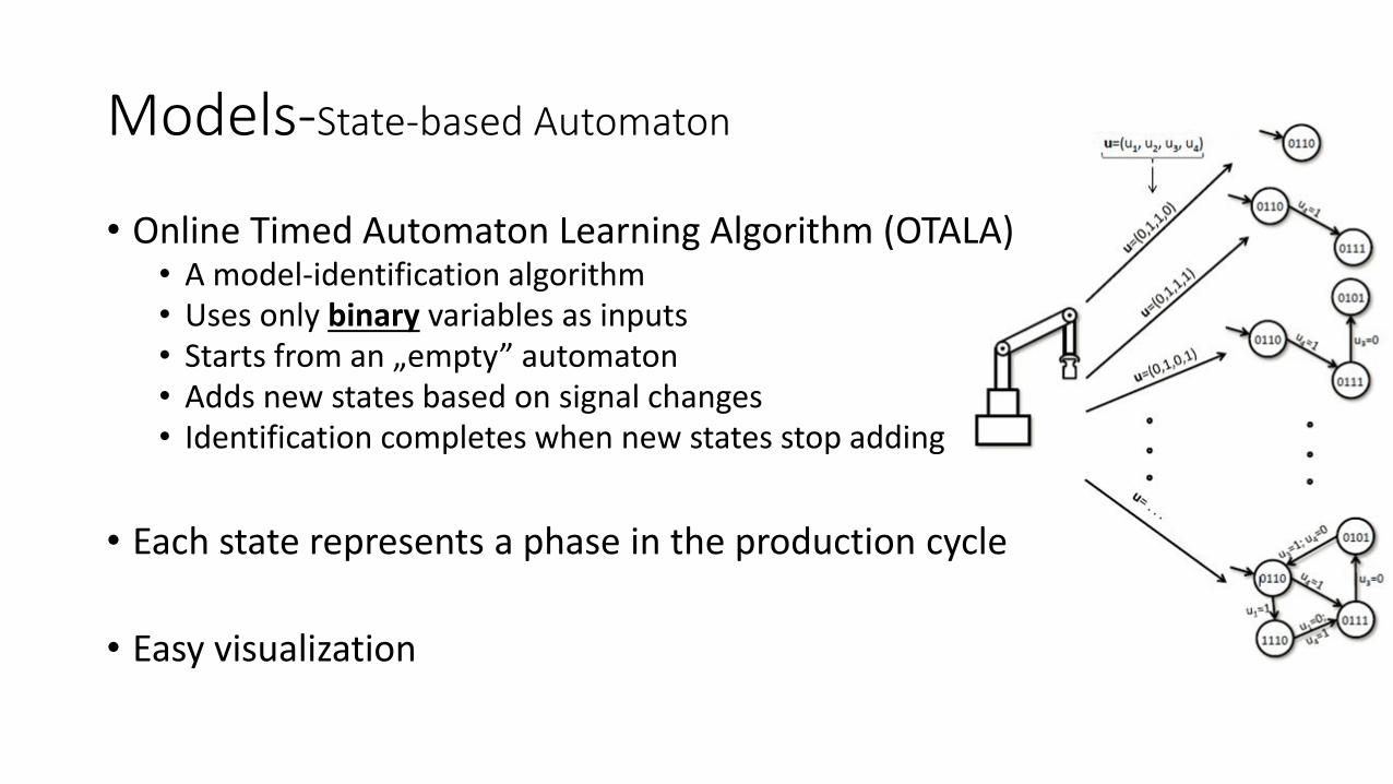
Models-State-based Automaton

• Online Timed Automaton Learning Algorithm (OTALA)• A model-identification algorithm• Uses only binary variables as inputs• Starts from an „empty” automaton• Adds new states based on signal changes• Identification completes when new states stop adding

• Each state represents a phase in the production cycle

• Easy visualization

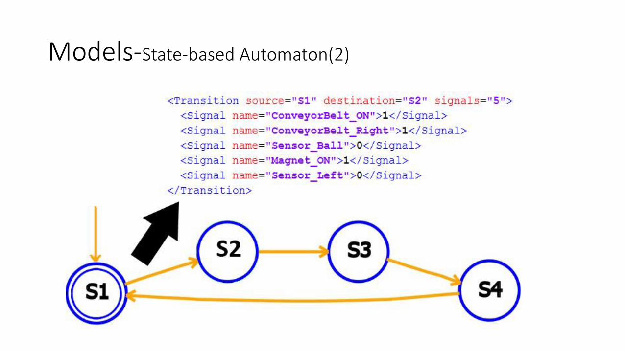
Models-State-based Automaton(2)

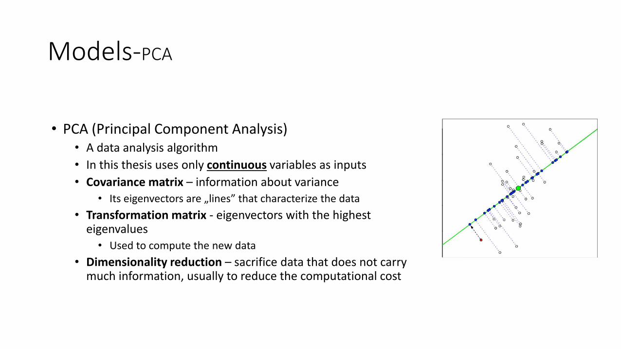
Models-PCA

• PCA (Principal Component Analysis)• A data analysis algorithm

• In this thesis uses only continuous variables as inputs

• Covariance matrix – information about variance• Its eigenvectors are „lines” that characterize the data

• Transformation matrix - eigenvectors with the highest eigenvalues• Used to compute the new data

• Dimensionality reduction – sacrifice data that does not carry much information, usually to reduce the computational cost

100110OTALA

PCA

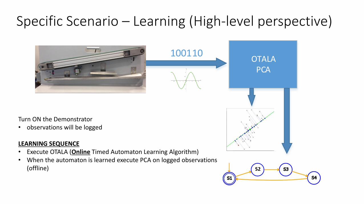
Specific Scenario – Learning (High-level perspective)

Turn ON the Demonstrator• observations will be logged

LEARNING SEQUENCE• Execute OTALA (Online Timed Automaton Learning Algorithm)• When the automaton is learned execute PCA on logged observations

(offline)

Observations and normal behaviour

( ) is the k-th observation containing only binary variables= 100110

NC = t=𝟏𝐅 is the continuous normal behaviour, where F is the total number of observations used to represent itu

C

(t)

( ) is the k-th observation containing only continuous variables=

uB

(k)

uC

(k)

( , ) is the k-th observationu(k) = 100110

N = t=𝟏𝐅 𝐮(t) is the normal behaviour, where F is the total number of observations used to represent it

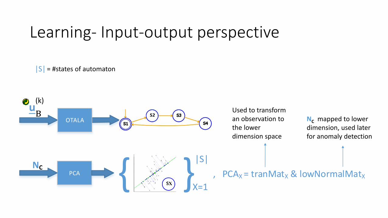
Learning- Input-output perspective

|S| = #states of automaton

Used to transforman observation to the lowerdimension space

NC mapped to lowerdimension, used laterfor anomaly detection

PCA

OTALA

NC { }X=1

|S|

, PCAX = tranMatX & lowNormalMatX

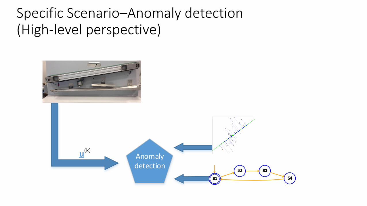
Specific Scenario–Anomaly detection(High-level perspective)

Anomalydetection

u(k)

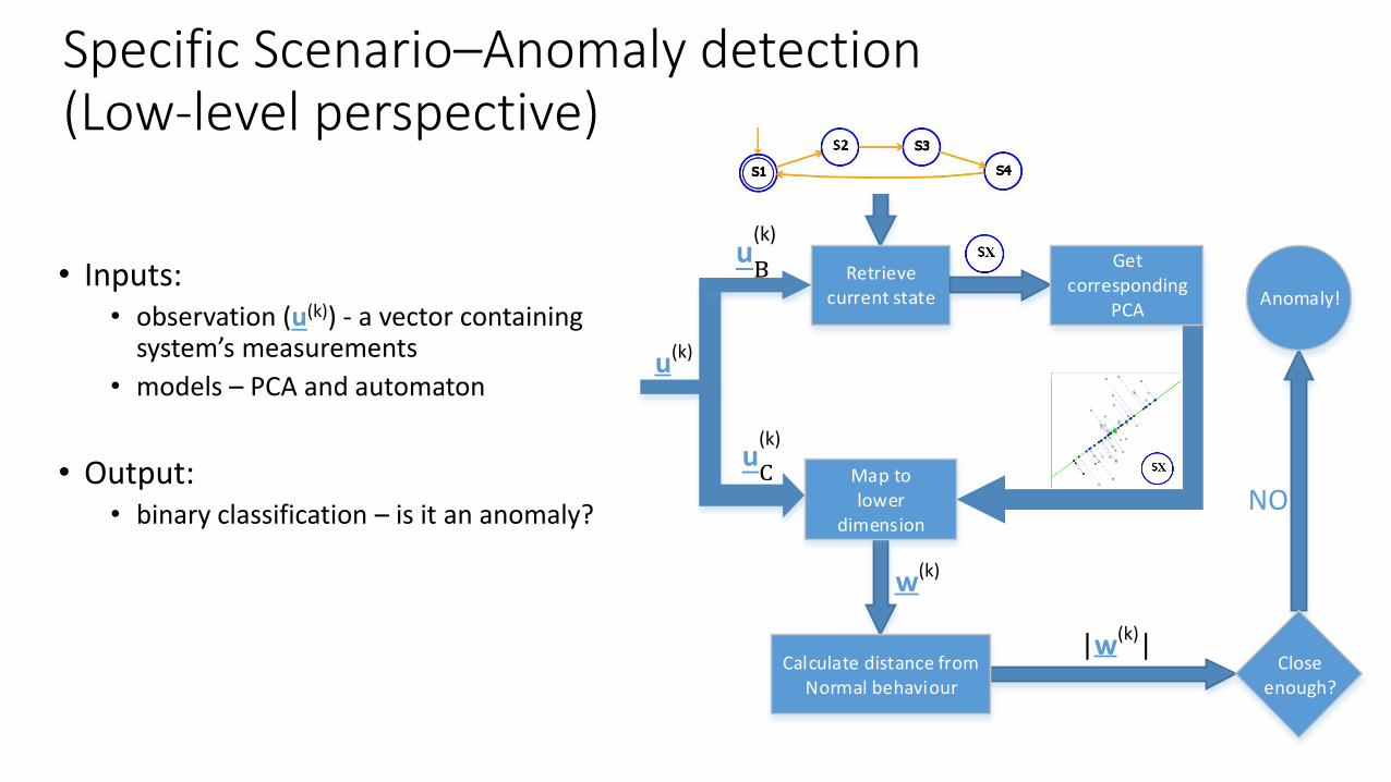
• Inputs: • observation (u(k)) - a vector containing

system’s measurements

• models – PCA and automaton

• Output:• binary classification – is it an anomaly?

Specific Scenario–Anomaly detection(Low-level perspective)

Retrieve current state

Map tolower

dimension

Calculate distance fromNormal behaviour

Close enough?

NO

Anomaly!

u(k)

Get corresponding

PCA

w(k)

|w(k)|

|𝒘| =

𝑖=1

𝑑

𝑤𝑖2

Classifier ( )

Euclideandistance from origin

Marrwaveletfunction

if (𝑓 𝒘 > 0)

then not anomaly

else anomaly Red – anomalyGreen – not anomaly

Close enough?

𝑓 𝒘 =2

3𝜎𝜋14

∗ 1 −|𝒘|

𝜎2∗ 𝑒−𝒘

2𝜎2

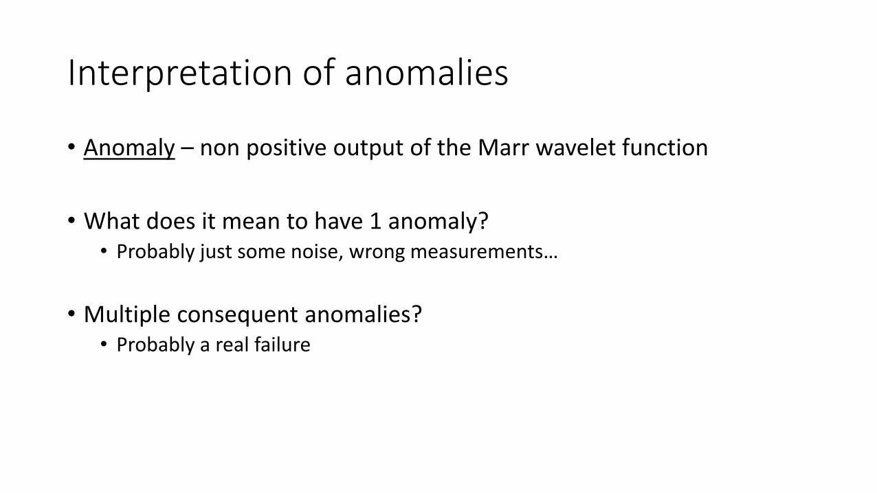
Interpretation of anomalies

• Anomaly – non positive output of the Marr wavelet function

• What does it mean to have 1 anomaly?• Probably just some noise, wrong measurements…

• Multiple consequent anomalies?• Probably a real failure

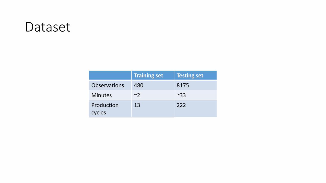
Dataset

Training set Testing set

Observations 480 8175

Minutes ~2 ~33

Productioncycles

13 222

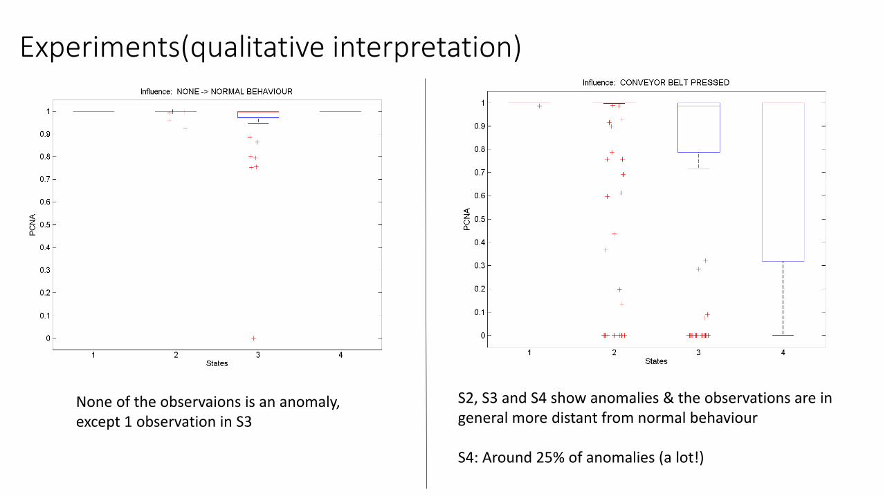
None of the observaions is an anomaly,except 1 observation in S3

S2, S3 and S4 show anomalies & the observations are ingeneral more distant from normal behaviour

S4: Around 25% of anomalies (a lot!)

Experiments(qualitative interpretation)

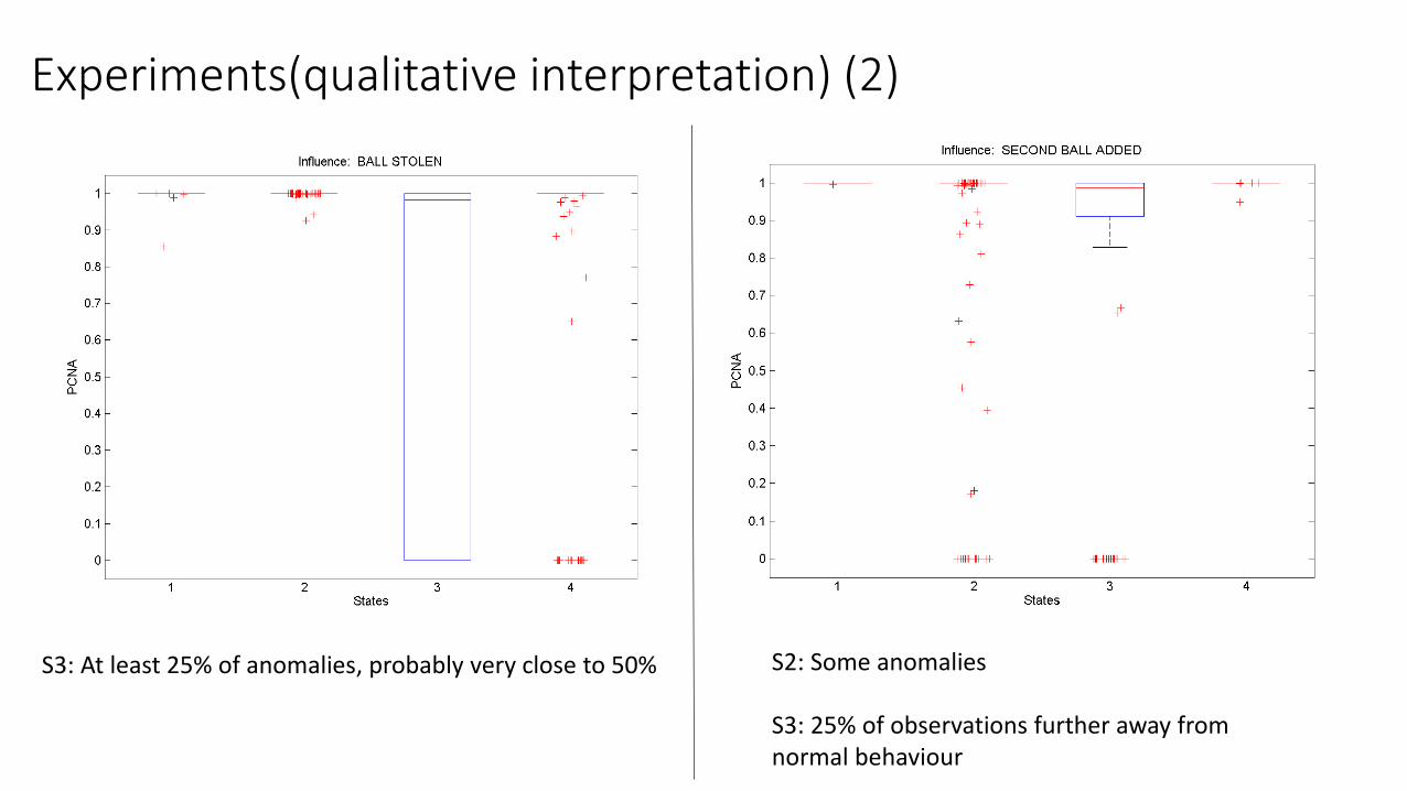
S3: At least 25% of anomalies, probably very close to 50% S2: Some anomalies

S3: 25% of observations further away fromnormal behaviour

Experiments(qualitative interpretation) (2)

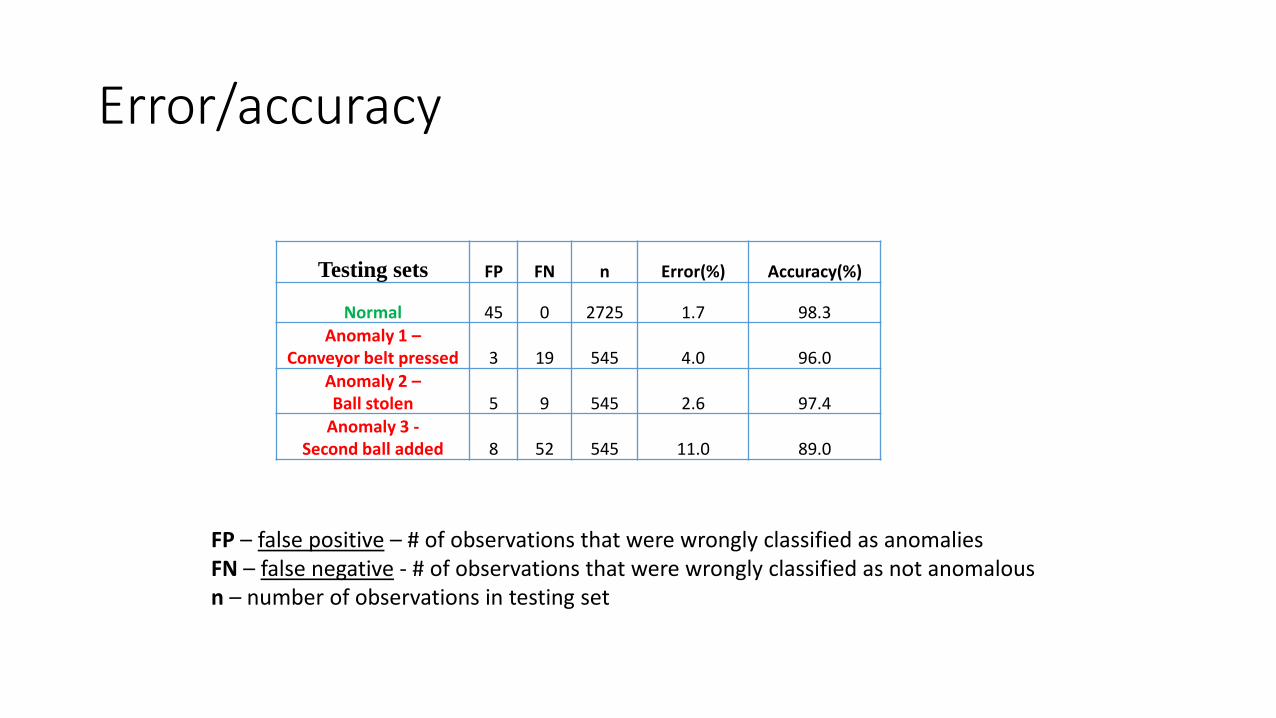
Error/accuracy

Testing sets FP FN n Error(%) Accuracy(%)

Normal 45 0 2725 1.7 98.3Anomaly 1 –

Conveyor belt pressed 3 19 545 4.0 96.0Anomaly 2 –Ball stolen 5 9 545 2.6 97.4

Anomaly 3 -Second ball added 8 52 545 11.0 89.0

FP – false positive – # of observations that were wrongly classified as anomaliesFN – false negative - # of observations that were wrongly classified as not anomalousn – number of observations in testing set

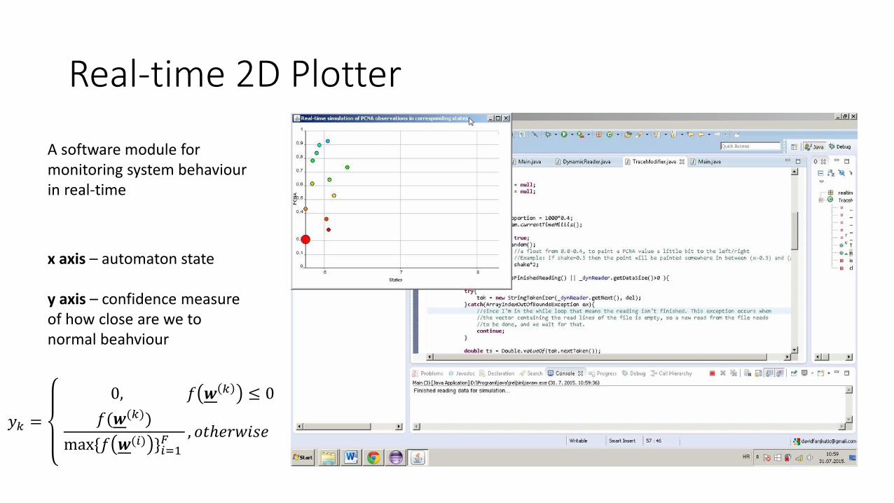
Real-time 2D Plotter

A software module for monitoring system behaviourin real-time

x axis – automaton state

y axis – confidence measureof how close are we to normal beahviour

𝑦𝑘 =

0, 𝑓 𝒘 𝑘 ≤ 0

𝑓(𝒘(𝑘))

max{𝑓 𝒘(𝑖) }𝑖=1𝐹, 𝑜𝑡ℎ𝑒𝑟𝑤𝑖𝑠𝑒

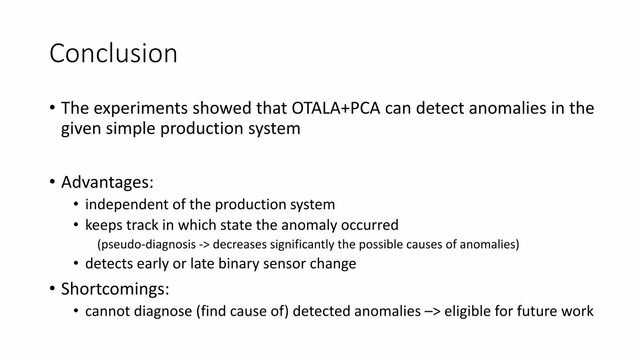
Conclusion

• The experiments showed that OTALA+PCA can detect anomalies in the given simple production system

• Advantages:• independent of the production system

• keeps track in which state the anomaly occurred(pseudo-diagnosis -> decreases significantly the possible causes of anomalies)

• detects early or late binary sensor change

• Shortcomings:• cannot diagnose (find cause of) detected anomalies –> eligible for future work

La presente tesi è prodotto dello scambio internazionale

presso la Hochschule-Ostwestfalen Lin a Lemgo, Germania

in collaborazione con

Infine

Grazie per l’attenzione