Embed Size (px)
Citation preview
European Finite Element Fair 4
ETH Zurich, 2-3 June 2006
A natural finite element for axisymmetric problem
Francois Dubois
CNAM Paris and University Paris South, Orsay
conjoint work with
Stefan Duprey
University Henri Poincare Nancy and EADS Suresnes.
A natural finite element for axisymmetric problem
1) Axi-symmetric model problem
2) Axi-Sobolev spaces
3) Discrete formulation
4) Numerical results for an analytic test case
5) About Clement’s interpolation
6) Numerical analysis
7) Conclusion
ETH Zurich, 2-3 June 2006
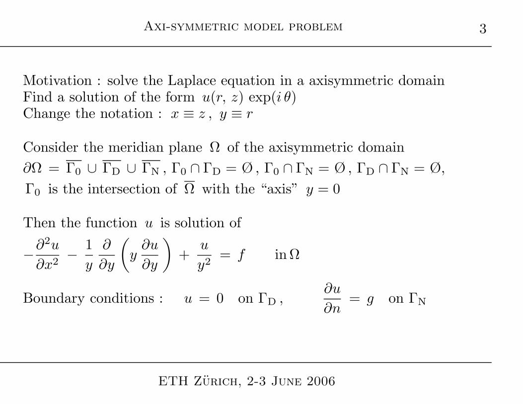
Axi-symmetric model problem
Motivation : solve the Laplace equation in a axisymmetric domainFind a solution of the form u(r, z) exp(i θ)Change the notation : x ≡ z , y ≡ r
Consider the meridian plane Ω of the axisymmetric domain
∂Ω = Γ0 ∪ ΓD ∪ ΓN , Γ0 ∩ ΓD = Ø , Γ0 ∩ ΓN = Ø , ΓD ∩ ΓN = Ø,
Γ0 is the intersection of Ω with the “axis” y = 0
Then the function u is solution of
−∂2u
∂x2− 1
y
∂
∂y
(y
∂u
∂y
)+
u
y2= f inΩ
Boundary conditions : u = 0 on ΓD ,∂u
∂n= g on ΓN
ETH Zurich, 2-3 June 2006
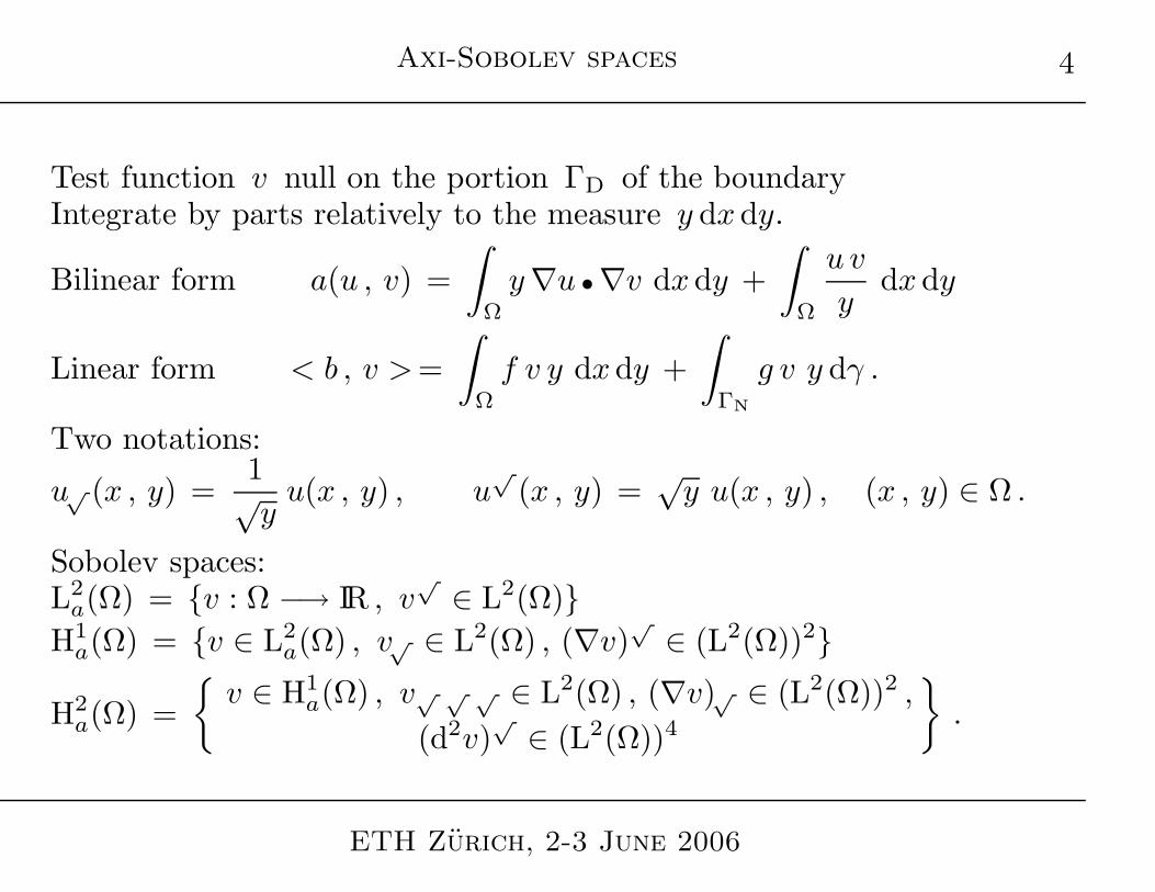
Axi-Sobolev spaces
Test function v null on the portion ΓD of the boundaryIntegrate by parts relatively to the measure y dxdy.
Bilinear form a(u , v) =
∫
Ω
y∇u •∇v dxdy +
∫
Ω
u v
ydxdy
Linear form < b , v >=
∫
Ω
f v y dxdy +
∫
ΓN
g v y dγ .
Two notations:
u√ (x , y) =1√y
u(x , y) , u√
(x , y) =√
y u(x , y) , (x , y) ∈ Ω .
Sobolev spaces:L2
a(Ω) = v : Ω −→ IR , v√
∈ L2(Ω)H1
a(Ω) = v ∈ L2a(Ω) , v√ ∈ L2(Ω) , (∇v)
√∈ (L2(Ω))2
H2a(Ω) =
v ∈ H1
a(Ω) , v√ √ √ ∈ L2(Ω) , (∇v)√ ∈ (L2(Ω))2 ,
(d2v)√
∈ (L2(Ω))4
.
ETH Zurich, 2-3 June 2006
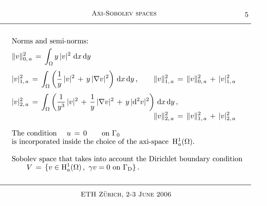
Axi-Sobolev spaces
Norms and semi-norms:
‖v‖20, a =
∫
Ω
y |v|2 dxdy
|v|21, a =
∫
Ω
(1
y|v|2 + y |∇v|2
)dxdy , ‖v‖2
1, a = ‖v‖20, a + |v|21, a
|v|22, a =
∫
Ω
(1
y3|v|2 +
1
y|∇v|2 + y |d2v|2
)dxdy ,
‖v‖22, a = ‖v‖2
1, a + |v|22, a
The condition u = 0 on Γ0
is incorporated inside the choice of the axi-space H1a(Ω).
Sobolev space that takes into account the Dirichlet boundary conditionV = v ∈ H1
a(Ω) , γv = 0 on ΓD .
ETH Zurich, 2-3 June 2006
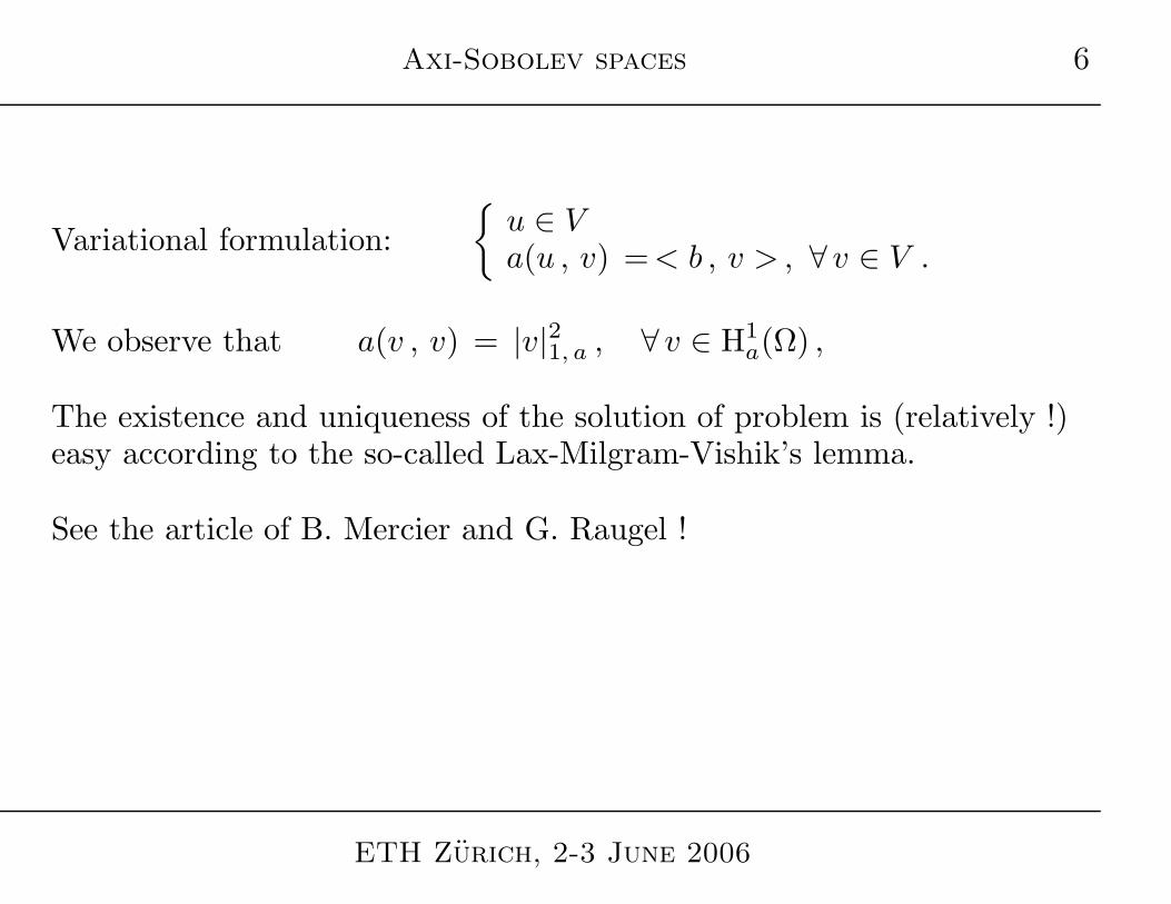
Axi-Sobolev spaces
Variational formulation:
u ∈ Va(u , v) =< b , v > , ∀ v ∈ V .
We observe that a(v , v) = |v|21, a , ∀ v ∈ H1a(Ω) ,
The existence and uniqueness of the solution of problem is (relatively !)easy according to the so-called Lax-Milgram-Vishik’s lemma.
See the article of B. Mercier and G. Raugel !
ETH Zurich, 2-3 June 2006
Discrete formulation
Very simple, but fundamental remark
Consider v(x , y) =√
y (a x + b y + c) , (x , y) ∈ K ∈ T 2 ,
Then we have√
y ∇v(x , y) =(a y ,
1
2(a x + 3b y + c)
).
P1 : the space of polynomials of total degree less or equal to 1
We have v√ ∈ P1 =⇒ (∇v)√
∈ (P1)2 .
A two-dimensional conforming mesh TT 0 set of vertices
T 1 set of edges
T 2 set of triangular elements.
ETH Zurich, 2-3 June 2006
Discrete formulation
Linear space P√
1 = v, v√ ∈ P1.
Degrees of freedom < δS , v > for v regular, S ∈ T 0 : < δS , v >= v√ (S)
Proposition 1. Unisolvance property.K ∈ T 2 be a triangle of the mesh T ,
Σ the set of linear forms < δS , • >, S ∈ T 0 ∩ ∂K
P√
1 defined above.
Then the triple (K , Σ , P√
1 ) is unisolvant.
Proposition 2. Conformity of the axi-finite element
The finite element (K , Σ , P√
1 ) is conforming in space C0(Ω).
Proposition 3. Conformity in the axi-space H1a(Ω).
The discrete space H√
T is included in the axi-space H1a(Ω) :H
√
T ⊂ H1a(Ω) .
ETH Zurich, 2-3 June 2006
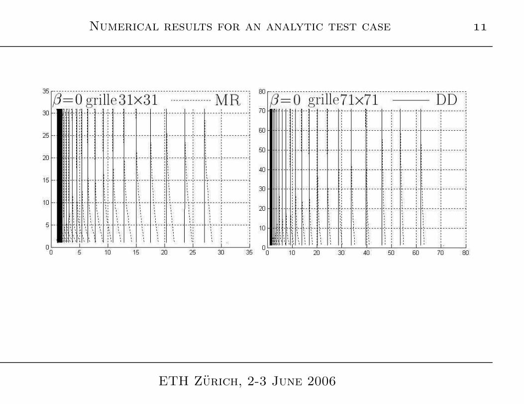
Numerical results for an analytic test case
Ω =]0, 1[2 , ΓD = Ø
Parameters α > 0, β > 0,
Right hand side: f (y, x) ≡ yα
[(α2 − 1
) xβ
y2+ β(β − 1)xβ−2
]
Neumann datum:g(x, y) = α if y = 1, −βyαxβ−1 if x = 0, βyα if x = 1.
Solution: u(x, y) ≡ yαxβ .
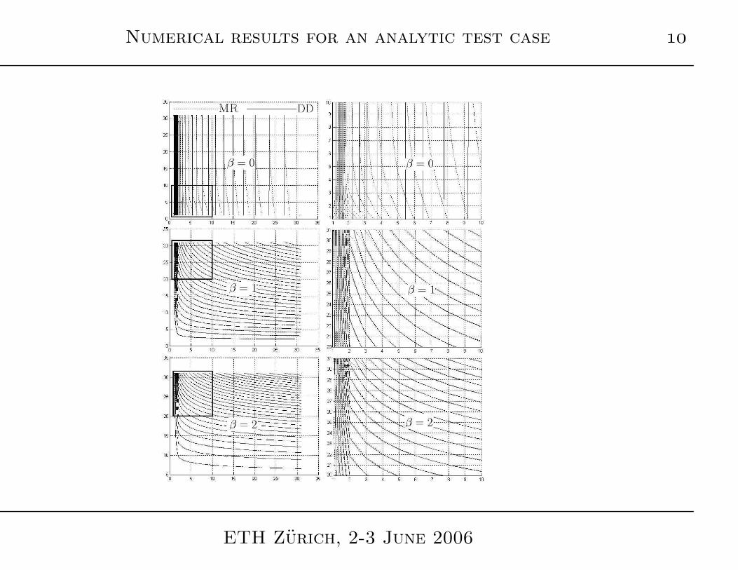
Comparison betweenthe present method (DD)the use of classical P1 finite elements (MR)
ETH Zurich, 2-3 June 2006
Numerical results for an analytic test case
ETH Zurich, 2-3 June 2006
Numerical results for an analytic test case
ETH Zurich, 2-3 June 2006
Numerical results for an analytic test case
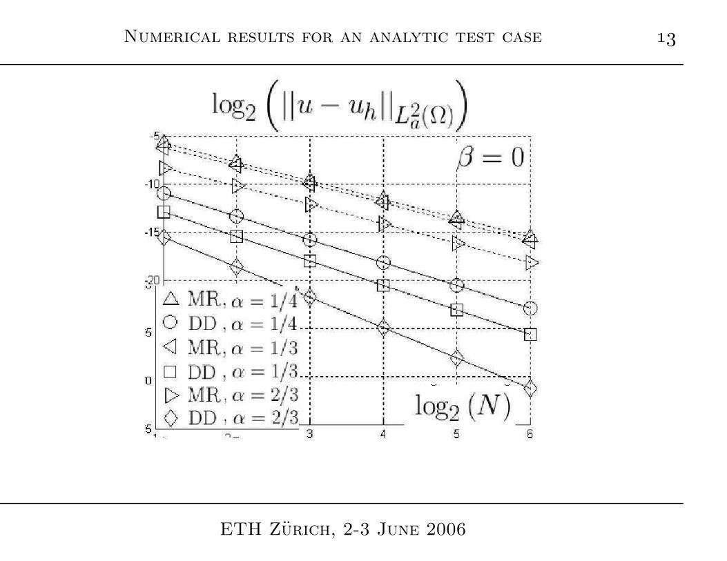
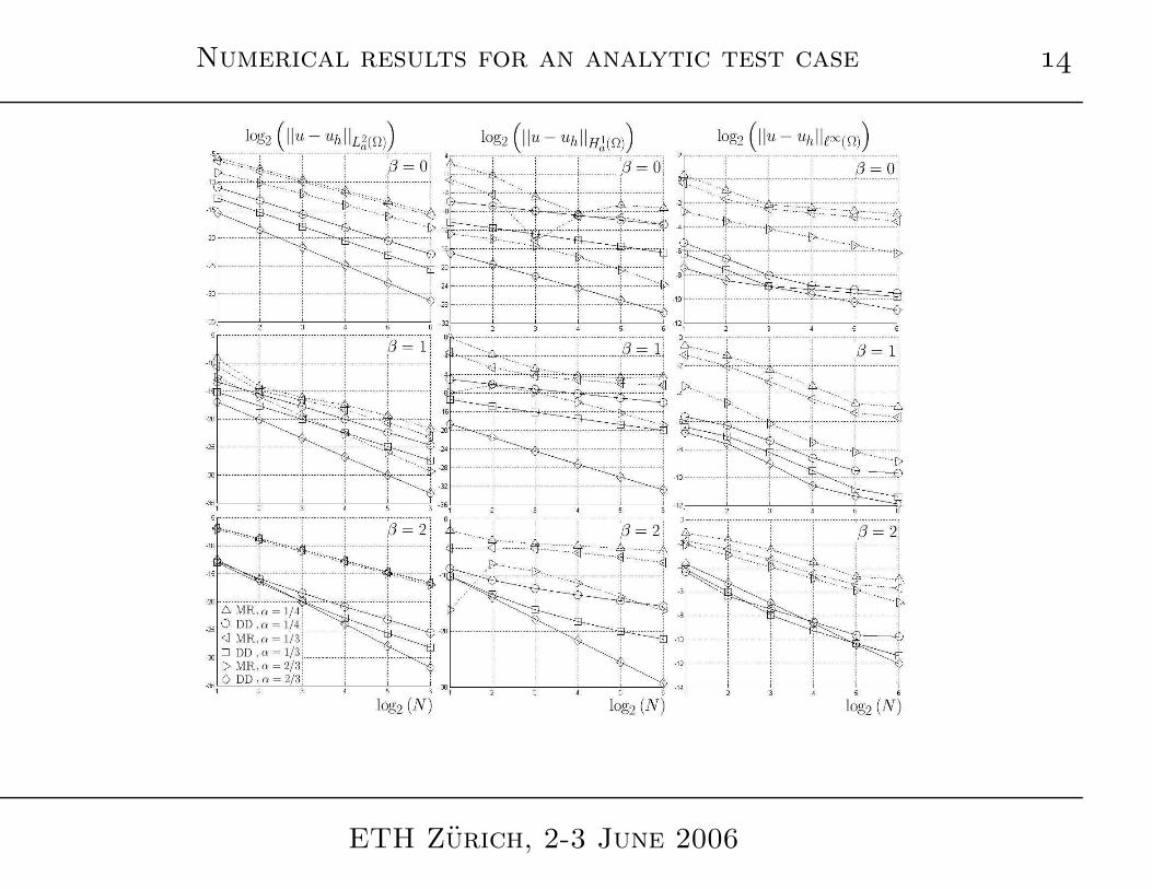
Numerical study of the convergence properties
Test cases :α = 1/4, α = 1/3, α = 2/3β = 0, β = 1, β = 2
Three norms: ‖v‖0, a |v|1, a ‖v‖ℓ∞
Order of convergence easy (?) to see.
Example : β = 0 and α = 2/3:our axi-finite element has a rate of convergence ≃ 3 for the ‖•‖0, a norm.
Synthesis of these experiments:
same order of convergence than with the classical approach
errors much more smaller!
ETH Zurich, 2-3 June 2006
Numerical results for an analytic test case
ETH Zurich, 2-3 June 2006
Numerical results for an analytic test case
ETH Zurich, 2-3 June 2006
Analysis ?
Discrete space for the approximation of the variational problem:
VT = H√
T ∩ V .
Discrete variational formulation:
uT ∈ VTa(uT , v) =< b , v > , ∀ v ∈ VT .
Estimate the error ‖u − uT ‖1, a
Study the interpolation error ‖u − ΠT u ‖1, a
What is the interpolate ΠT u ??
Proposition 4. Lack of regularity.Hypothesis: u ∈ H2
a(Ω).Then u√ belongs to the space H1(Ω) and ‖u√ ‖1, Ω ≤ C ‖u‖2, a
ETH Zurich, 2-3 June 2006
Analysis ?
Introduce v ≡ u√ . Small calculus: ∇v = − 1
2y√
yu∇y +
1√y∇u .
Then
∫
Ω
|v|2 dxdy ≤∫
Ω
1
y|u|2 dxdy ≤ C ‖u‖2
2, a
∫
Ω
|∇v|2 dxdy ≤ 2
∫
Ω
( 1
4y3|u|2 +
1
y|∇u|2
)dxdy ≤ C ‖u‖2
2, a .
Derive (formally !) two times:
d2v =3
4 y2√
yu∇y •∇y − 1
y√
y∇u •∇y +
1√y
d2u
Even if u is regular, v has no reason to be continuous.
ETH Zurich, 2-3 June 2006
About Clement’s interpolation
S
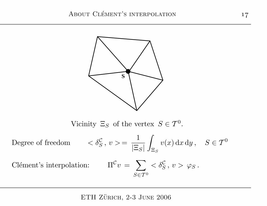
Vicinity ΞS of the vertex S ∈ T 0.
Degree of freedom < δCS , v >=1
|ΞS |
∫
ΞS
v(x) dxdy , S ∈ T 0
Clement’s interpolation: ΠCv =∑
S∈T 0
< δCS , v > ϕS .
ETH Zurich, 2-3 June 2006
About Clement’s interpolation
K
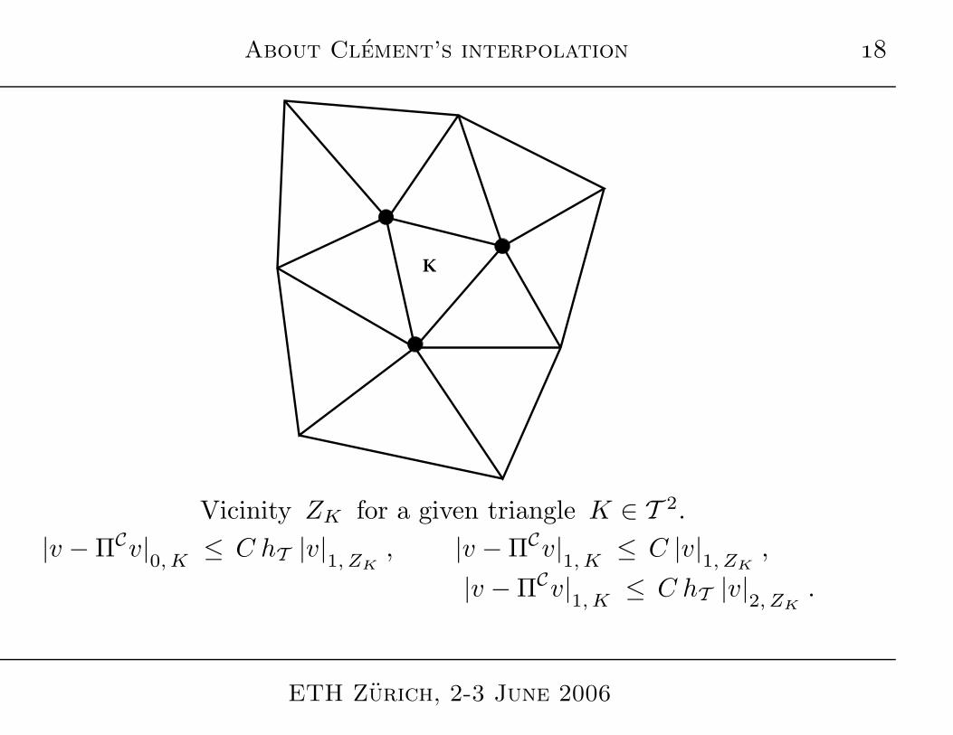
Vicinity ZK for a given triangle K ∈ T 2.
|v − ΠCv|0, K
≤ C hT |v|1, ZK
, |v − ΠCv|1, K
≤ C |v|1, ZK
,
|v − ΠCv|1, K
≤ C hT |v|2, ZK
.
ETH Zurich, 2-3 June 2006
Numerical analysis
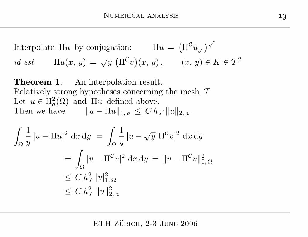
Interpolate Πu by conjugation: Πu =(ΠCu√
)√
id est Πu(x, y) =√
y(ΠCv
)(x, y) , (x, y) ∈ K ∈ T 2
Theorem 1. An interpolation result.Relatively strong hypotheses concerning the mesh TLet u ∈ H2
a(Ω) and Πu defined above.Then we have ‖u − Πu‖1, a ≤ C hT ‖u‖2, a .
∫
Ω
1
y|u − Πu|2 dxdy =
∫
Ω
1
y|u −√
y ΠCv|2 dxdy
=
∫
Ω
|v − ΠCv|2 dxdy = ‖v − ΠCv‖20, Ω
≤ C h2T |v|21, Ω
≤ C h2T ‖u‖2
2, a
ETH Zurich, 2-3 June 2006
Numerical analysis
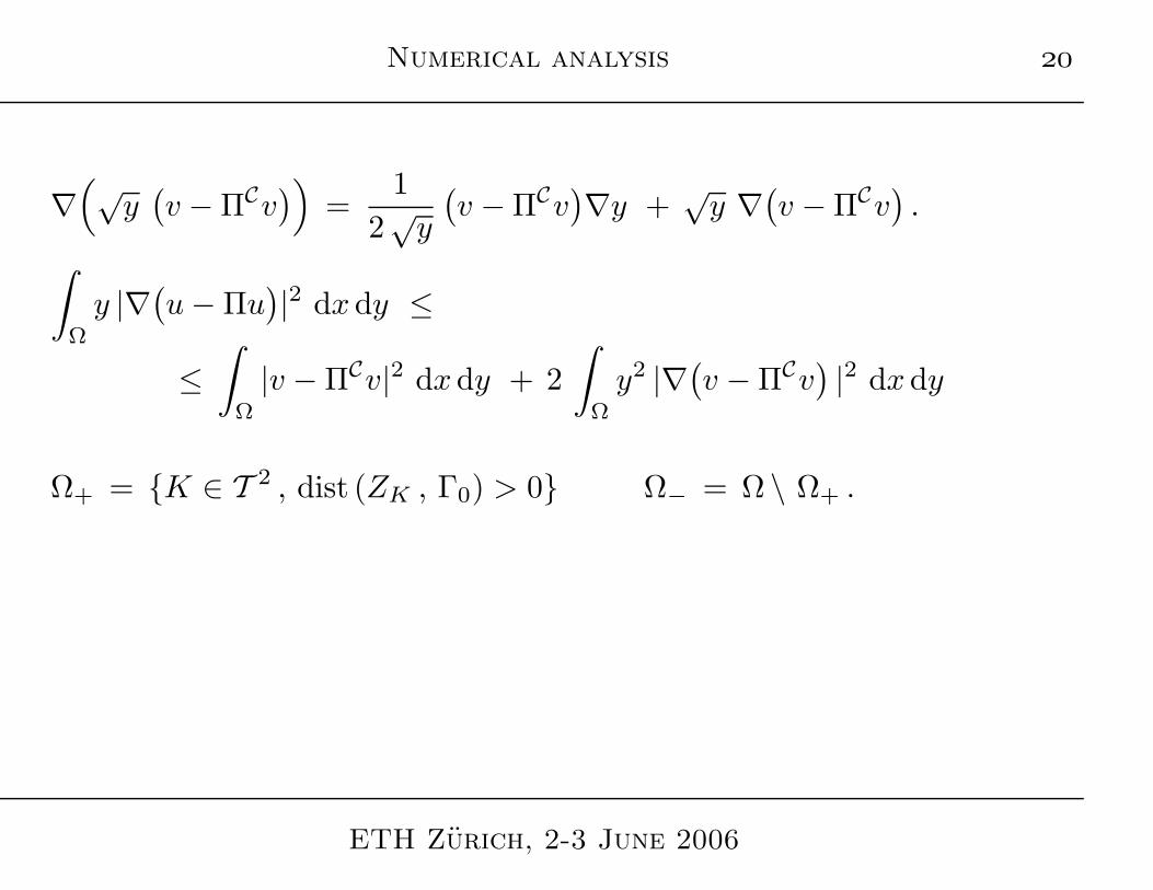
∇(√
y(v − ΠCv
))=
1
2√
y
(v − ΠCv
)∇y +
√y ∇
(v − ΠCv
).
∫
Ω
y |∇(u − Πu
)|2 dxdy ≤
≤∫
Ω
|v − ΠCv|2 dxdy + 2
∫
Ω
y2 |∇(v − ΠCv
)|2 dxdy
Ω+ = K ∈ T 2 , dist (ZK , Γ0) > 0 Ω− = Ω \ Ω+ .
ETH Zurich, 2-3 June 2006
Numerical analysis
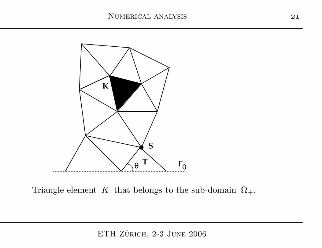
S
0ΓTθ
K
Triangle element K that belongs to the sub-domain Ω+.
ETH Zurich, 2-3 June 2006
Numerical analysis
Theorem 2. First order approximationrelatively strong hypotheses concerning the mesh Tu solution of the continuous problem: u ∈ H2
a(Ω) ,Then we have ‖u − uT ‖1, a ≤ C hT ‖u‖2, a .
Proof: classical with Cea’s lemma!
ETH Zurich, 2-3 June 2006
Conclusion
“Axi-finite element”
Interpolation properties founded of the underlying axi-Sobolev space
First numerical tests: good convergence properties
Numerical analysis based on Mercier-Raugel contribution (1982)
See also Gmati (1992), Bernardi et al. (1999)
May be all the material presented here is well known ?!
ETH Zurich, 2-3 June 2006