An Introduction to knitr and RMarkdown

https://github.com/sahirbhatnagar/knitr-tutorial

Sahir Bhatnagar

August 12, 2015

McGill Univeristy

Acknowledgements

• Toby, Matthieu, Vaughn,

Ary

• Maxime Turgeon (Windows)

• Kevin McGregor (Mac)

• Greg Voisin

• Don Knuth (TEX)

• Friedrich Leisch (Sweave)

• Yihui Xie (knitr)

• John Gruber (Markdown)

• John MacFarlane (Pandoc)

• You

2/36

Disclaimer #1

I don’t work for, nor am I an author of any of these packages. I’m just a

messenger. 3/36

Disclaimer #2

• Material for this tutorial comes from many sources. For a complete

list see: https://github.com/sahirbhatnagar/knitr-tutorial

• Alot of the content in these slides are based on these two books

4/36

Objectives for today

• Create a reproducible

document (pdf, html)

5/36

Objectives for today

• Create a reproducible

document (pdf, html)

5/36

C’est parti

6/36

What?

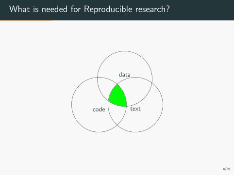
What is needed for Reproducible research?

code

data

text

8/36

Why?

Why should we care about RR?

For Science

Standard to judge

scientific claims

Avoid duplication

Cumulative

knowledge

development

For You

Better work

habits

Better teamwork

Changes

are easier

Higher re-

search impact

10/36

Why should we care about RR?

For Science

Standard to judge

scientific claims

Avoid duplication

Cumulative

knowledge

development

For You

Better work

habits

Better teamwork

Changes

are easier

Higher re-

search impact

10/36

001-motivating-example

A Motivating Example

Demonstrate: 001-motivating-example

12/36

How?

Tools for Reproducible Research

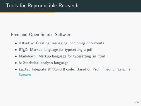
Free and Open Source Software

• RStudio: Creating, managing, compiling documents

• LATEX: Markup language for typesetting a pdf

• Markdown: Markup language for typesetting an html

• R: Statistical analysis language

• knitr: Integrate LATEXand R code. Based on Prof. Friedrich Leisch’s

Sweave

14/36

knitr

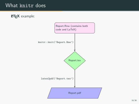
What knitr does

LATEX example:

Report.Rnw (contains both

code and LaTeX)

Report.tex

knitr::knit(’Report.Rnw’)

Report.pdf

latex2pdf(’Report.tex’)

16/36

What knitr does

LATEX example:

Report.Rnw (contains both

code and LaTeX)

Report.tex

knitr::knit(’Report.Rnw’)

Report.pdf

latex2pdf(’Report.tex’)

16/36

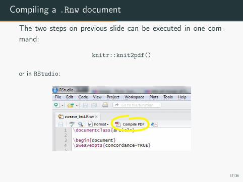
Compiling a .Rnw document

The two steps on previous slide can be executed in one com-

mand:

knitr::knit2pdf()

or in RStudio:

17/36

Incorporating R code

• Insert R code in a Code Chunk starting with

<< >>=

and ending with

@

In RStudio:

18/36

Example 1: Show code and results

<<example-code-chunk-name, echo=TRUE>>=

x <- rnorm(50)

mean(x)

@

produces

x <- rnorm(50)

mean(x)

## [1] 0.031

19/36

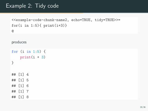
Example 2: Tidy code

<<example-code-chunk-name2, echo=TRUE, tidy=TRUE>>=

for(i in 1:5){ print(i+3)}

@

produces

for (i in 1:5) {

print(i + 3)

}

## [1] 4

## [1] 5

## [1] 6

## [1] 7

## [1] 8

20/36

Example 2.2: don’t show code

<<example-code-chunk-name3, echo=FALSE>>=

for(i in 1:5){ print(i+3)}

@

produces

## [1] 4

## [1] 5

## [1] 6

## [1] 7

## [1] 8

21/36

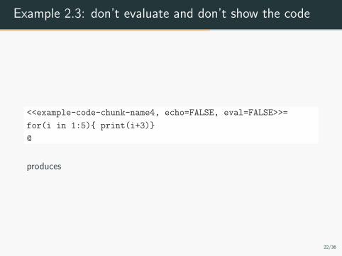
Example 2.3: don’t evaluate and don’t show the code

<<example-code-chunk-name4, echo=FALSE, eval=FALSE>>=

for(i in 1:5){ print(i+3)}

@

produces

22/36

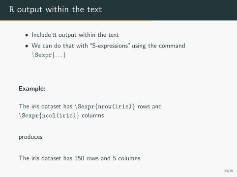
R output within the text

• Include R output within the text

• We can do that with“S-expressions”using the command

\Sexpr{. . .}

Example:

The iris dataset has \Sexpr{nrow(iris)} rows and

\Sexpr{ncol(iris)} columns

produces

The iris dataset has 150 rows and 5 columns

23/36

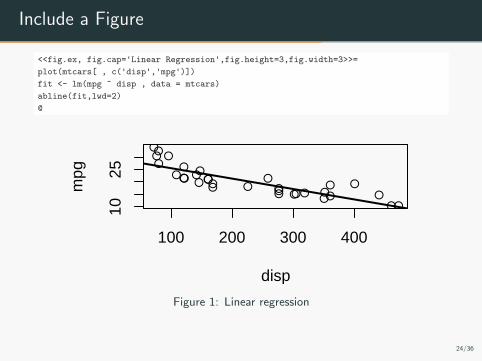
Include a Figure

<<fig.ex, fig.cap='Linear Regression',fig.height=3,fig.width=3>>=plot(mtcars[ , c('disp','mpg')])fit <- lm(mpg ~ disp , data = mtcars)

abline(fit,lwd=2)

@

●●● ●●●●

●●●● ●●●

●●●

●●

●

●

●● ●

●

● ●●

●●

●

●

100 200 300 400

1025

disp

mpg

Figure 1: Linear regression

24/36

Include a Table

<<table.ex, results='asis'>>=library(xtable)

tab <- xtable(iris[1:5,1:5],caption='Sample of Iris data')print(tab, include.rownames=FALSE)

@

library(xtable)

tab <- xtable(iris[1:5,1:5], caption = 'Sample of Iris data')print(tab, include.rownames = F)

Sepal.Length Sepal.Width Petal.Length Petal.Width Species

5.10 3.50 1.40 0.20 setosa

4.90 3.00 1.40 0.20 setosa

4.70 3.20 1.30 0.20 setosa

4.60 3.10 1.50 0.20 setosa

5.00 3.60 1.40 0.20 setosa

Table 1: Sample of Iris data

25/36

RMarkdown

Markdown: HTML without knowing HTML

27/36

R + Markdown = RMarkdown

28/36

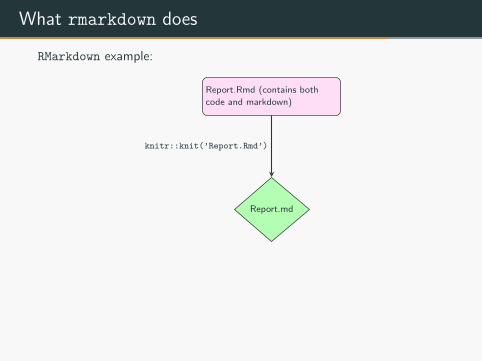
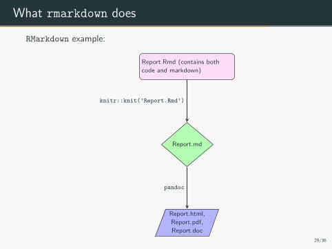
What rmarkdown does

RMarkdown example:

Report.Rmd (contains both

code and markdown)

Report.md

knitr::knit(’Report.Rmd’)

Report.html,

Report.pdf,

Report.doc

pandoc

29/36

What rmarkdown does

RMarkdown example:

Report.Rmd (contains both

code and markdown)

Report.md

knitr::knit(’Report.Rmd’)

Report.html,

Report.pdf,

Report.doc

pandoc

29/36

Compiling a .Rmd document

The two steps on previous slide can be executed in one com-

mand:

rmarkdown::render()

or in RStudio:

30/36

Final Remarks

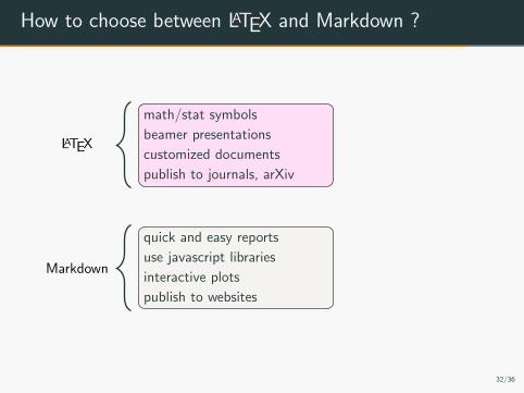
How to choose between LATEX and Markdown ?

math/stat symbols tecccccc

beamer presentations teccccc

customized documents tecccc

publish to journals, arXiv

quick and easy reportstkkk

use javascript libraries tekkt

interactive plots texkkkkjjt

publish to websites

LATEX

Markdown

32/36

33/36

Always Remember ...

Reproducibility ∝ 1

copy paste

34/36

Is the juice worth the squeeze?

35/36

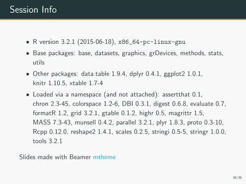
Session Info

• R version 3.2.1 (2015-06-18), x86_64-pc-linux-gnu

• Base packages: base, datasets, graphics, grDevices, methods, stats,

utils

• Other packages: data.table 1.9.4, dplyr 0.4.1, ggplot2 1.0.1,

knitr 1.10.5, xtable 1.7-4

• Loaded via a namespace (and not attached): assertthat 0.1,

chron 2.3-45, colorspace 1.2-6, DBI 0.3.1, digest 0.6.8, evaluate 0.7,

formatR 1.2, grid 3.2.1, gtable 0.1.2, highr 0.5, magrittr 1.5,

MASS 7.3-43, munsell 0.4.2, parallel 3.2.1, plyr 1.8.3, proto 0.3-10,

Rcpp 0.12.0, reshape2 1.4.1, scales 0.2.5, stringi 0.5-5, stringr 1.0.0,

tools 3.2.1

Slides made with Beamer mtheme

36/36