Rhelogy, Diffusion and PlasticCorrelations in Jammed

Suspensions

Arka Prabha Roy

PhD Thesis Proposal

Committee:

Craig E. Maloney (Advisor)

Jacobo BielakMichael Widom

Alan J. H. McGaughey

Mechanics, Materials and Computing

Department of Civil and Environmental Engineering

Carnegie Mellon University, Pittsburgh

April 1, 2015

Abstract

We perform computer simulations of amorphous, frictionless soft discs to

study the effect of strain rates, γ, on the microscopic dynamics and plastic-

ity of jammed suspensions. We study the rate of energy dissipation, single

particle diffusivity and spatial correlations and relate these to the non-linear

rheology observed above the yield stress, σY . At small γ, the system responds

in a bursty, intermittent way, reminiscent of other dynamically critical systems

with a power law distribution of energy dissipation rates. With increasing γ

the intermittency vanishes. At high γ there is a crossover from short time bal-

listic motion to long time diffusive motion. The effective diffusion coefficient,

D, scales as γ in a non-trivial way, D ∝ γ−1/3. We also show a character-

istic length scale, ξ, observed both in the velocity field and the long time

(plastic) displacement field, grows with decreasing γ in a similar fashion fol-

lowing ξ ∝ γ−1/3, and finally saturates at the system size. Both shear strain

and instantaneous strain-rate show pronounced long ranged correlations with

quadrupolar symmetry. We interpret these correlations as arising in response

to shear transformations.

i

Contents

1 Introduction 1

2 Numerical Model 72.1 Particle Scale Dynamics . . . . . . . . . . . . . . . . . . . . . . . . . 82.2 Simulation Protocol . . . . . . . . . . . . . . . . . . . . . . . . . . . . 11

3 Rheology and Dissipated Energy 133.1 Rheology . . . . . . . . . . . . . . . . . . . . . . . . . . . . . . . . . . 14

3.1.1 Stress vs Strain for Various Shearing Rate . . . . . . . . . . . 163.2 Instantaneous Energy Dissipation Rate . . . . . . . . . . . . . . . . . 19

3.2.1 Quasistatic Scaling of Γ Distribution . . . . . . . . . . . . . . 203.2.2 Strain Rate Dependence . . . . . . . . . . . . . . . . . . . . . 22

4 Displacement Statistics 244.1 Diffusive Behavior . . . . . . . . . . . . . . . . . . . . . . . . . . . . . 26

5 Spatial Correlations 325.1 The Eshelby Response . . . . . . . . . . . . . . . . . . . . . . . . . . 335.2 Displacement and Strain Correlation . . . . . . . . . . . . . . . . . . 365.3 Velocity and Strain-rate Correlation . . . . . . . . . . . . . . . . . . . 48

6 Summary and Future Work 57

A Fourier space representation 66

ii

List of Figures

1.1 Three different types of soft amorphous materials: (a) Colloidal sus-pension (Weeks Soft Matter Laboratory, Emory University), (b) Oil-water emulsion (Blair Lab, Georgetown University), (c) Foam (MartinVan Hecke Laboratory, Leiden University) . . . . . . . . . . . . . . . 3

1.2 Non-Newtonian rheology below jamming (φ < φc) and Yield stressbehavior above jamming (φ > φc) in a microgel system [1]. Differentcolors correspond to different densities which are collapsed onto twomaster curves. . . . . . . . . . . . . . . . . . . . . . . . . . . . . . . . 4

1.3 Scaled stress vs strain rate data for two different types of emulsion:high viscosity oil in water-glycerol (closed symbol) and low viscosity oilin water (open symbol). Dashed line corresponds to Herschel-Bulkleyfit using the elasto-hydrodynmic model. [2] . . . . . . . . . . . . . . . 5

2.1 Repulsive Interaction between two disc like particles. . . . . . . . . . 92.2 Primary Simulation cell in 2D space. Simple shear is applied along x

direction. . . . . . . . . . . . . . . . . . . . . . . . . . . . . . . . . . 112.3 Strain Controlled periodic box with Lees Edwards boundary condition

for a simple shear application. . . . . . . . . . . . . . . . . . . . . . . 12

3.1 Shear stress (σ) vs shear rate (γ) above and below φJ , φ = 0.9 andφ = 0.8 for L = 20. The green straight line has a slope of 1, whichindicates the Newtonian rheology. Inset: Viscosity (η) vs γ with thestraight line of slope -1 . . . . . . . . . . . . . . . . . . . . . . . . . . 15

3.2 Macroscopic shear stress (σ) vs strain (γ) for γ = 10−7, very close tothe quasi-static limit for L = 40. . . . . . . . . . . . . . . . . . . . . . 16

3.3 σ vs γ for 3 different strain rates γ = 8× [10−7, 10−5, 10−3]. . . . . . . 173.4 Flow stress (σ) vs strain rate (γ) for a jammed system(φ = 0.9),

L = 40. The dashed line has a slope of 1/3. . . . . . . . . . . . . . . 18

iii

3.5 Experimental results for foams and bubbles from (a) Michael Dennin'sgroup [37] and (b) Martin Van Hecke's Group [10]. The black line in(a) has a slope of 1/3 and the black curve in (b) is a Herschel Bulkleyfit with an exponent of 0.35. . . . . . . . . . . . . . . . . . . . . . . . 18

3.6 Instantaneous energy dissipated per unit strain (Γ) vs strain (γ) forγ = 10−7. . . . . . . . . . . . . . . . . . . . . . . . . . . . . . . . . . 20

3.7 Probability distribution of Γ for 4 different γ = [1, 2, 4, 8]× 10−7 nearthe yield stress regime. . . . . . . . . . . . . . . . . . . . . . . . . . . 21

3.8 Probability Distribution of Γ vs Γ scaled by rate for 4 different γ =[1, 2, 4, 8]× 10−7. The peaks corresponding to the elastic loading nearthe slow γ limit is clearly visible. . . . . . . . . . . . . . . . . . . . . 22

3.9 Γ vs γ for 3 different strain rates, γ = 8× [10−7, 10−5, 10−3]. . . . . . 223.10 Probability distribution of Γ for a spectrum of strain rates, γ ∈ [1 ×

10−7, 8 × 10−3]. Blue curve denote slow γ, which is near QS regimeand Red denote high γ where the system has no time for relaxation. . 23

4.1 (a) Total displacement field and (b) Non-affine contribution only ofthe displacement field defined over ∆γ = 1% for γ = 10−6. . . . . . . 25

4.2 MSD in the transverse direction as a function of ∆γ for γ = 10−4,L = 20. Inset:〈∆y2〉/∆γ vs ∆γ. For large ∆γ, ∆y2/∆γ is constant. . 27

4.3 Scaled second moment (〈∆y2〉/∆γ) vs strain window (∆γ) for differentrates, γ = [1, 2, 4, 8, 10, 20, 40, 80, 100, 200, 400, 800] × 10−5, L = 40.Red correspond to a fast rate (γ = 8× 10−3) and violet correspond toa intermediate rate (γ = 1× 10−5). . . . . . . . . . . . . . . . . . . . 28

4.4 (a) Scaled second moment and (b) scaled fourth moment of the dis-placement distribution for different rates, γ = [1, 2, 4, 8, 10, 20, 40, 80, 100, 200, 400, 800, 1000, 2000, 4000, 8000, 10000, 20000, 40000, 80000]×10−7, L = 40. Red correspond to a fast rate (γ = 8× 10−3) and bluecorrespond to a slow rate (γ = 1× 10−7). . . . . . . . . . . . . . . . . 28

4.5 (a) Non-Gaussian parameter (α) and (b) kurtosis (γ2 = 1/α−1) of thedisplacement distribution for different rates, γ = [1, 2, 4, 8, 10, 20, 40, 80, 100, 200, 400, 800, 1000, 2000, 4000, 8000, 10000, 20000, 40000, 80000]×10−7, L = 40. Red correspond to a fast rate (γ = 8× 10−3) and bluecorrespond to a slow rate (γ = 1 × 10−7). The black dashed line in(a) corresponds to α = 1 and in (b) corresponds to γ2 ∝ 1/∆γ. . . . . 29

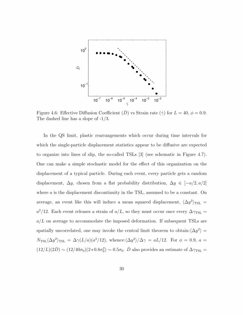
4.6 Effective Diffusion Coefficient (D) vs Strain rate (γ) for L = 40, φ =0.9. The dashed line has a slope of -1/3. . . . . . . . . . . . . . . . . 30

iv

4.7 (a) Horizontal and (b) Vertical displacements during a horizontal slipevent, (c) Schematic representation of the non-affine displacementsparallel to a slip line of length L over a plastic zone of width h and adisplacement discontinuity a. [3] . . . . . . . . . . . . . . . . . . . . . 31

5.1 Left : The perturbation due to a local plastic stress is equivalent tothe perturbation due to the two set of force dipoles; Right : Responsein stress field under the action of the force dipole. [4] . . . . . . . . . 34

5.2 Non-affine displacement field at the onset of a plastic event in a metal-lic glass. Quadrupolar structure confirms the Eshelby flip event. [5] . 35

5.3 Transverse displacement, ∆y, incurred between γ = 1.2 and γ = 1.225(∆γ = 0.025 ∼ 1/L) for (a) Slowly sheared system (γ = 8×10−7) and(b) Rapidly sheared system (γ = 8 × 10−3). The displacement fieldis obtained by interpolating the particle displacements on a regularmesh-grid at the reference configuration when γ = 1.2. . . . . . . . . 37

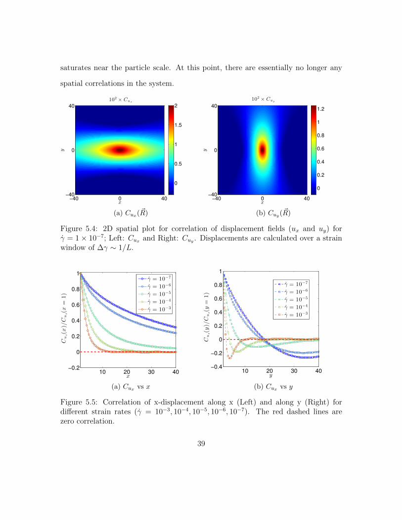
5.4 2D spatial plot for correlation of displacement fields (ux and uy) forγ = 1×10−7; Left: Cux and Right: Cuy . Displacements are calculatedover a strain window of ∆γ ∼ 1/L. . . . . . . . . . . . . . . . . . . . 39

5.5 Correlation of x-displacement along x (Left) and along y (Right) fordifferent strain rates (γ = 10−3, 10−4, 10−5, 10−6, 10−7). The red dashedlines are zero correlation. . . . . . . . . . . . . . . . . . . . . . . . . . 39

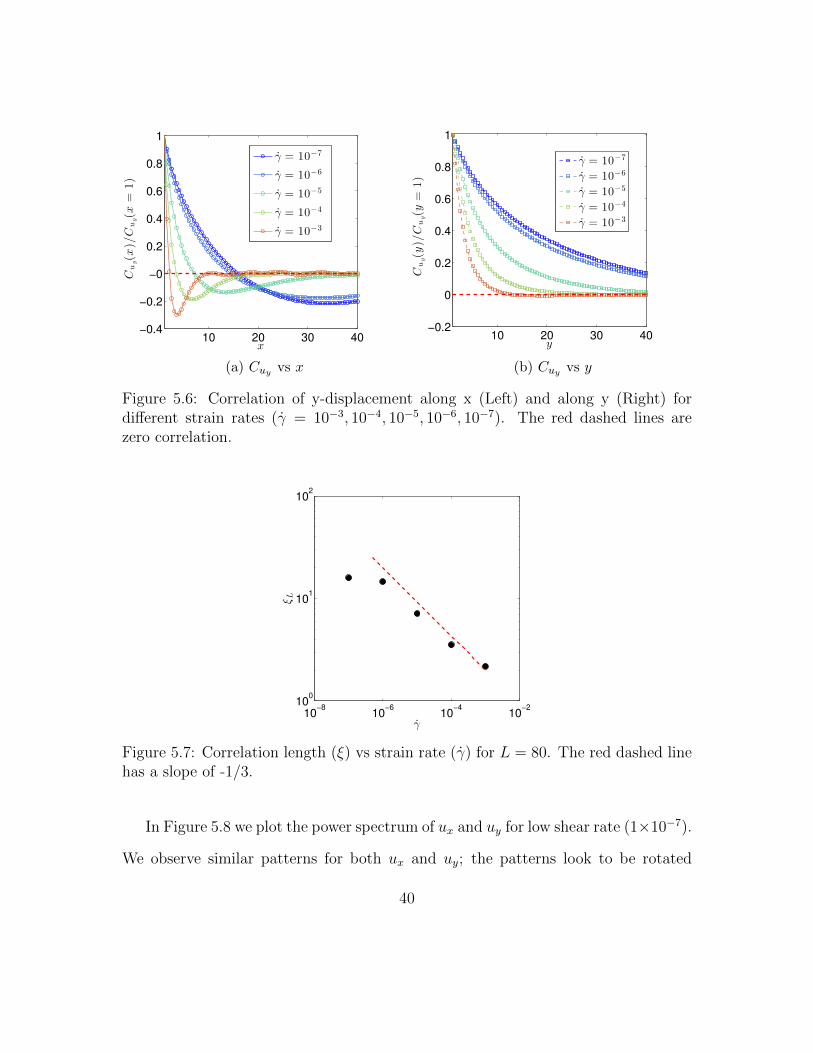
5.6 Correlation of y-displacement along x (Left) and along y (Right) fordifferent strain rates (γ = 10−3, 10−4, 10−5, 10−6, 10−7). The red dashedlines are zero correlation. . . . . . . . . . . . . . . . . . . . . . . . . . 40

5.7 Correlation length (ξ) vs strain rate (γ) for L = 80. The red dashedline has a slope of -1/3. . . . . . . . . . . . . . . . . . . . . . . . . . . 40

5.8 Power of x-displacement (Left) and y-displacement (Right) for γ = 1×10−7 and displacement calculated over a strain interval of ∆γ ∼ 1/L;Left: Sux and Right: Suy . A logarithmic(base10) color scale is used toshow the magnitude. . . . . . . . . . . . . . . . . . . . . . . . . . . . 41

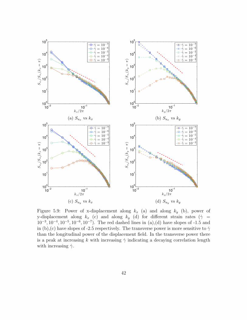
5.9 Power of x-displacement along kx (a) and along ky (b), power of y-displacement along kx (c) and along ky (d) for different strain rates(γ = 10−3, 10−4, 10−5, 10−6, 10−7). The red dashed lines in (a),(d)have slopes of -1.5 and in (b),(c) have slopes of -2.5 respectively. Thetransverse power is more sensitive to γ than the longitudinal powerof the displacement field. In the transverse power there is a peak atincreasing k with increasing γ indicating a decaying correlation lengthwith increasing γ. . . . . . . . . . . . . . . . . . . . . . . . . . . . . . 42

v

5.10 Correlation of gradients of x and y-displacement for γ = 1×10−7; (a):C∂xux , (b): C∂yux , (c): C∂xuy , (d): C∂yuy . . . . . . . . . . . . . . . . . 44

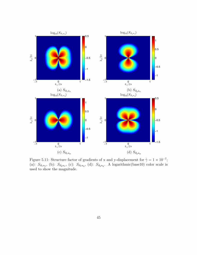
5.11 Structure factor of gradients of x and y-displacement for γ = 1×10−7;(a): S∂xux , (b): S∂yux , (c): S∂xuy , (d): S∂yuy . A logarithmic(base10)color scale is used to show the magnitude. . . . . . . . . . . . . . . . 45

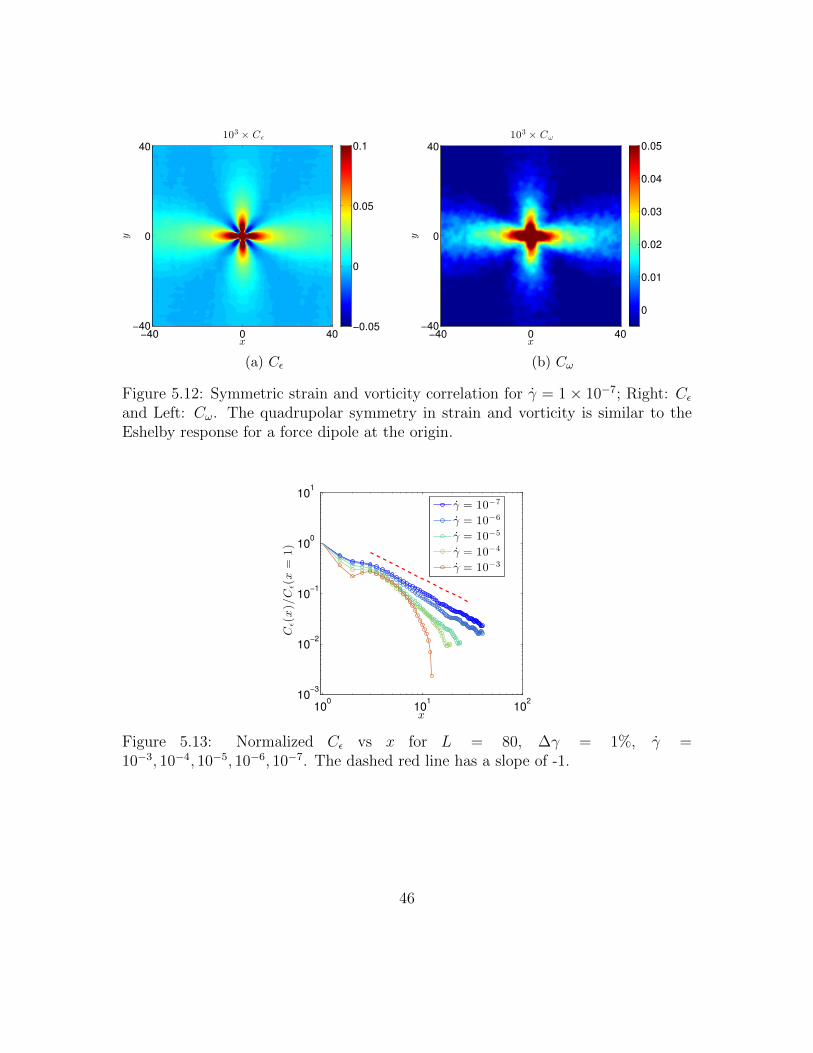
5.12 Symmetric strain and vorticity correlation for γ = 1 × 10−7; Right:Cε and Left: Cω. The quadrupolar symmetry in strain and vorticityis similar to the Eshelby response for a force dipole at the origin. . . . 46

5.13 Normalized Cε vs x for L = 80, ∆γ = 1%, γ = 10−3, 10−4, 10−5, 10−6, 10−7.The dashed red line has a slope of -1. . . . . . . . . . . . . . . . . . . 46

5.14 Structure factor of strain (Sε) vorticity (Sω) for γ = 1 × 10−7; Left:Sε and Right: Sω. A logarithmic(base10) color scale is used to showthe magnitude. . . . . . . . . . . . . . . . . . . . . . . . . . . . . . . 47

5.15 Power of strain (Sε) along kx, for γ = 1× [10−7, 10−6, 10−5, 10−4, 10−3].The red dashed line has a slope of -2/3 . . . . . . . . . . . . . . . . . 47

5.16 The y-velocity (vy) of particles before an event (Left) and after theevent has occurred (Right) are plotted for a slow rate (γ = 8× 10−7). 49

5.17 A typical image for the y-velocities (vy) for a fast sheared system(γ = 8× 10−3). . . . . . . . . . . . . . . . . . . . . . . . . . . . . . . 50

5.18 Correlation of vertical velocity field (Cvy) for different γ : (a) slow(γ = 10−7) and (b) fast (γ = 10−3). . . . . . . . . . . . . . . . . . . . 50

5.19 Correlation of x velocity along x (a) and along y (b); Correlationof y velocity along x (c) and along y (d) for different strain rates(γ = 10−3, 10−4, 10−5, 10−6, 10−7). The red dashed lines are guide forzero correlation. . . . . . . . . . . . . . . . . . . . . . . . . . . . . . . 51

5.20 Correlation length vs strain rate for L = 80. The red dashed linehas a slope of -1/3. ξ′ is calculated by taking the minimum of thecorrelation functions plotted in Figure 5.19c. . . . . . . . . . . . . . . 52

5.21 Power spectrum of x-velocity (Left) and y-velocity (Right) for γ = 1×10−7. A logarithmic(base10) color scale is used to show the magnitude. 52

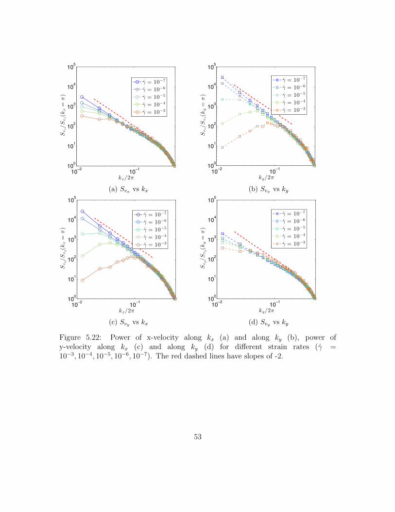
5.22 Power of x-velocity along kx (a) and along ky (b), power of y-velocityalong kx (c) and along ky (d) for different strain rates (γ = 10−3, 10−4, 10−5, 10−6, 10−7).The red dashed lines have slopes of -2. . . . . . . . . . . . . . . . . . 53

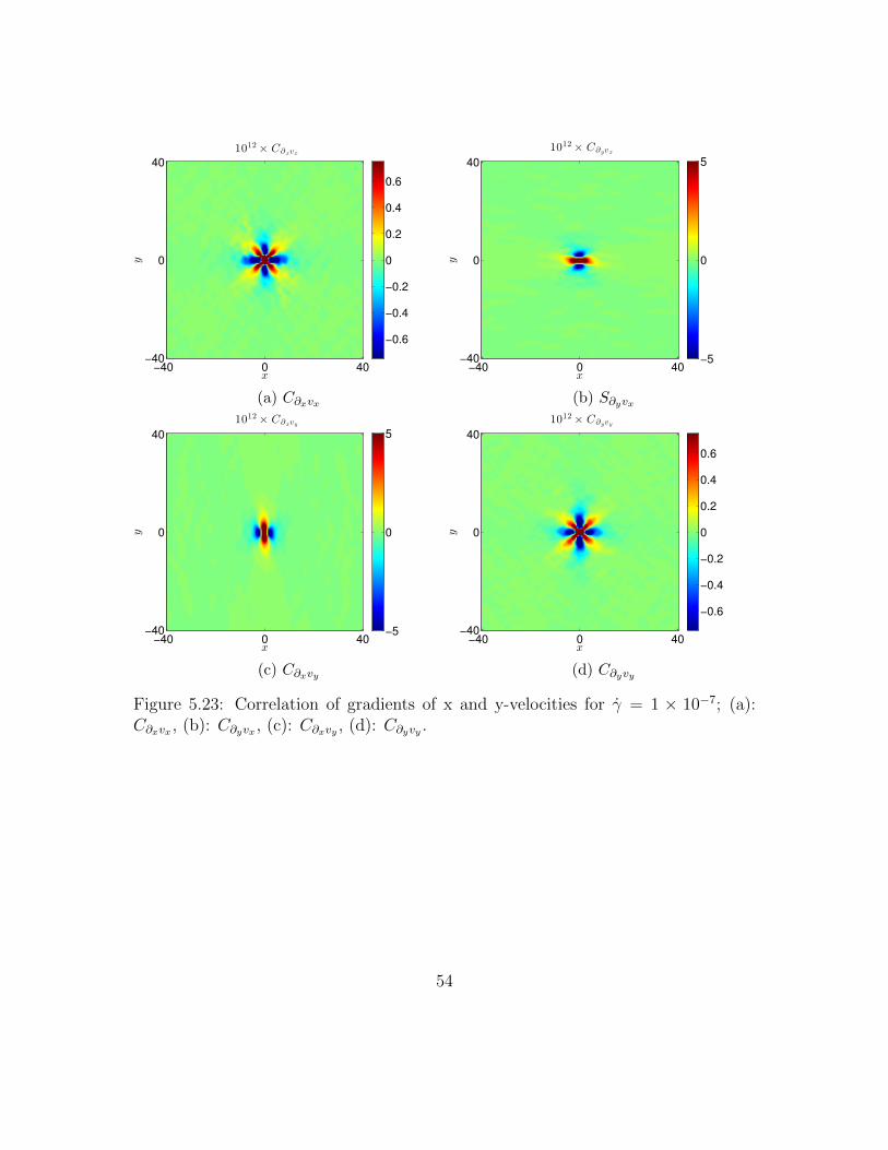
5.23 Correlation of gradients of x and y-velocities for γ = 1 × 10−7; (a):C∂xvx , (b): C∂yvx , (c): C∂xvy , (d): C∂yvy . . . . . . . . . . . . . . . . . . 54

5.24 Power spectrum of gradients of x and y-velocities for γ = 1 × 10−7;(a): S∂xvx , (b): S∂yvx , (c): S∂xvy , (d): S∂yvy . A logarithmic(base10)color scale is used to show the magnitude. . . . . . . . . . . . . . . . 55

vi

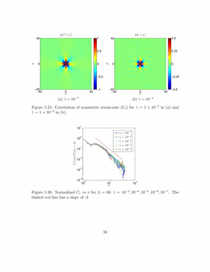
5.25 Correlation of symmetric strain-rate (Cε) for γ = 1× 10−7 in (a) andγ = 1× 10−3 in (b). . . . . . . . . . . . . . . . . . . . . . . . . . . . . 56

5.26 Normalized Cε vs x for L = 80, γ = 10−3, 10−4, 10−5, 10−6, 10−7. Thedashed red line has a slope of -2. . . . . . . . . . . . . . . . . . . . . 56

6.1 Stress vs strain rate for different damping constant for the Pair-Dragmodel. . . . . . . . . . . . . . . . . . . . . . . . . . . . . . . . . . . . 59

vii

Chapter 1

Introduction

1

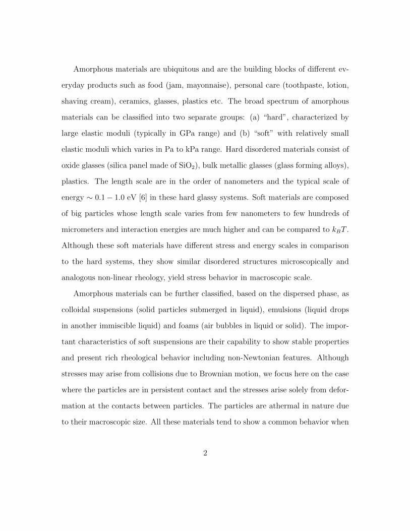
Amorphous materials are ubiquitous and are the building blocks of different ev-

eryday products such as food (jam, mayonnaise), personal care (toothpaste, lotion,

shaving cream), ceramics, glasses, plastics etc. The broad spectrum of amorphous

materials can be classified into two separate groups: (a) “hard”, characterized by

large elastic moduli (typically in GPa range) and (b) “soft” with relatively small

elastic moduli which varies in Pa to kPa range. Hard disordered materials consist of

oxide glasses (silica panel made of SiO2), bulk metallic glasses (glass forming alloys),

plastics. The length scale are in the order of nanometers and the typical scale of

energy ∼ 0.1− 1.0 eV [6] in these hard glassy systems. Soft materials are composed

of big particles whose length scale varies from few nanometers to few hundreds of

micrometers and interaction energies are much higher and can be compared to kBT .

Although these soft materials have different stress and energy scales in comparison

to the hard systems, they show similar disordered structures microscopically and

analogous non-linear rheology, yield stress behavior in macroscopic scale.

Amorphous materials can be further classified, based on the dispersed phase, as

colloidal suspensions (solid particles submerged in liquid), emulsions (liquid drops

in another immiscible liquid) and foams (air bubbles in liquid or solid). The impor-

tant characteristics of soft suspensions are their capability to show stable properties

and present rich rheological behavior including non-Newtonian features. Although

stresses may arise from collisions due to Brownian motion, we focus here on the case

where the particles are in persistent contact and the stresses arise solely from defor-

mation at the contacts between particles. The particles are athermal in nature due

to their macroscopic size. All these materials tend to show a common behavior when

2

the particles are densely packed. They can resist a finite amount of stress and act as

an elastic solid before flowing like a viscous fluid above a yield stress. The yield stress

behavior is exploited in various industries to make different consumer products like

solid ink, ceramic pastes etc., where it is often desirable for the materials to remain

solid yet flow at low stress when desired (e.g. squeezing toothpaste through a tube

or ketchup or mayonnaise through a bottle).

Figure 1.1: Three different types of soft amorphous materials: (a) Colloidal sus-pension (Weeks Soft Matter Laboratory, Emory University), (b) Oil-water emulsion(Blair Lab, Georgetown University), (c) Foam (Martin Van Hecke Laboratory, LeidenUniversity)

In the past few years many experimentalists [1, 2, 7–15] have studied different

classes of soft amorphous materials (foams, bubbles, microgel suspensions) in the

unjammed as well as jammed state and found interesting behavior with deformation

rate. Nordstrom et al. [1,13] have studied the motion of these dense microgel suspen-

sions in a microfluidic rheometer for varying shearing rates and have noticed different

dependence on shearing rates at the two sides of jamming transition (Figure 1.2).

Above the jamming transition, the system developed a yield stress. Below jamming,

the stress vanished at vanishing rate. In Martin Van Hecke group [7–10], they have

also observed nonlinear behavior of stress versus strain rate for a dense foam. Every

3

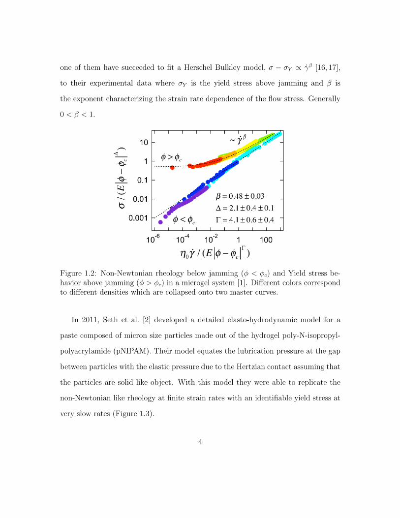
one of them have succeeded to fit a Herschel Bulkley model, σ − σY ∝ γβ [16, 17],

to their experimental data where σY is the yield stress above jamming and β is

the exponent characterizing the strain rate dependence of the flow stress. Generally

0 < β < 1.

Figure 1.2: Non-Newtonian rheology below jamming (φ < φc) and Yield stress be-havior above jamming (φ > φc) in a microgel system [1]. Different colors correspondto different densities which are collapsed onto two master curves.

In 2011, Seth et al. [2] developed a detailed elasto-hydrodynamic model for a

paste composed of micron size particles made out of the hydrogel poly-N-isopropyl-

polyacrylamide (pNIPAM). Their model equates the lubrication pressure at the gap

between particles with the elastic pressure due to the Hertzian contact assuming that

the particles are solid like object. With this model they were able to replicate the

non-Newtonian like rheology at finite strain rates with an identifiable yield stress at

very slow rates (Figure 1.3).

4

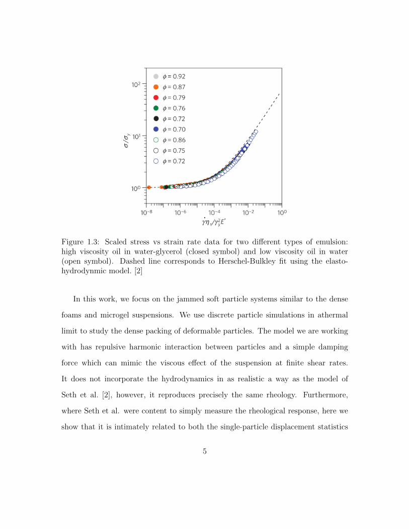
Figure 1.3: Scaled stress vs strain rate data for two different types of emulsion:high viscosity oil in water-glycerol (closed symbol) and low viscosity oil in water(open symbol). Dashed line corresponds to Herschel-Bulkley fit using the elasto-hydrodynmic model. [2]

In this work, we focus on the jammed soft particle systems similar to the dense

foams and microgel suspensions. We use discrete particle simulations in athermal

limit to study the dense packing of deformable particles. The model we are working

with has repulsive harmonic interaction between particles and a simple damping

force which can mimic the viscous effect of the suspension at finite shear rates.

It does not incorporate the hydrodynamics in as realistic a way as the model of

Seth et al. [2], however, it reproduces precisely the same rheology. Furthermore,

where Seth et al. were content to simply measure the rheological response, here we

show that it is intimately related to both the single-particle displacement statistics

5

(through the diffusion coefficient) and to the spatial structure of the resulting particle

rearrangements.

The objective of this PhD work is to investigate the effect of finite strain rates

on plastic deformation in amorphous soft materials via particle based numerical

simulation performed at zero temperature. In particular, we want to answer the the

question, “How are rheology, diffusivity, and spatial structure of the rearrangements

related?” We will show that all three of these are governed by a correlation length for

the rearrangements which diverges as the shearing rate vanishes in a way reminiscent

of other athermal driven systems.

We start with a description of the particle model and the simulation protocol in

Chapter 2.. In Chapter 3 we present the results for the shear rheology and the energy

dissipation and how it depends on the shearing rates. We find bursty, intermittent

behavior at very slow rates similar to the Quasistatic results for amorphous materials

[5,18–20] and uniform energy dissipation with constant stress vs strain response when

sheared rapidly. In Chapter 4 we study the displacement distributions and long time

particle diffusion for different shearing rates. In Chapter 5 we present our results for

the long time plastic correlations and short time instantaneous structural analysis.

In Chapter 6 we summarize the results, present preliminary data for future work,

and outline the remaining work for this PhD thesis.

6

Chapter 2

Numerical Model

7

In this chapter we introduce the numerical model used to perform the particle

based simulation. The important points to note here are:

1. All stresses come from persistent deformation at contact between the particles.

2. There is no thermal motion. If the system is not explicitly driven by external

deformation, it will remain at rest.

3. The precise form of the repulsion between the interacting particles is not impor-

tant. We use a harmonic repulsive contact force in the data reported here, but

have observed similar behavior with non-linear contact forces such as Hertzian

contacts.

4. The particles are perfectly circular disks, and there is no friction or adhe-

sion/attraction at the contacts.

To study the dynamic behavior of the system we drive the system using a simple

shear mechanism, under the assumption of overdamped dynamics, where the mass

of the particles does not play a role .

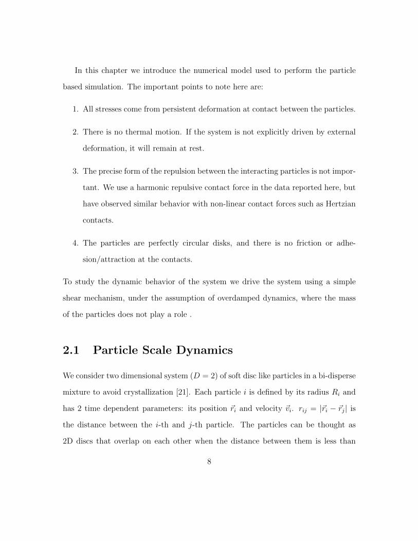
2.1 Particle Scale Dynamics

We consider two dimensional system (D = 2) of soft disc like particles in a bi-disperse

mixture to avoid crystallization [21]. Each particle i is defined by its radius Ri and

has 2 time dependent parameters: its position ~ri and velocity ~vi. rij = |~ri − ~rj| is

the distance between the i-th and j-th particle. The particles can be thought as

2D discs that overlap on each other when the distance between them is less than

8

the sum of their radii, rij < (Ri + Rj). In that case the overlap is measured as,

δij = (Ri + Rj) − rij. Diameter of the small particle is takel There are NL large

and NS small particles with NL : NS = 50 : 50. The size ratio of the particles are

1.4 [21], i.e., RL : RS = 1.4 : 1. All lengths are reported in units of the diameter of

the smaller particle σ0 = 2RS.

�ij

rij

U(rij) / �2ij

Figure 2.1: Repulsive Interaction between two disc like particles.

We use the so called “mean-field” version of the Durian bubble model [22]. In

this model, the particles experience two pairwise additive interactions based on their

overlap and dissipative mechanism. First, the elastic repulsion is modeled by a

harmonic potential U = kδ2 if δ < 0 and zero otherwise, where k is the elastic spring

constant between the particles. The elastic force on particle i due to particle j is,

~FEij =

∂U(rij)

∂~rj(2.1)

Thus, the total elastic force experienced by particle i due to its overlapping

contacts j is,

~FEi =

∑j

~FEij (2.2)

9

The second interaction is the viscous dissipation that is taken into account in a

mean-field fashion by the relative velocity defined with respect to the background

shear profile. This type of damping mechanism might be a realistic expression for

the drag experienced by a soap bubble (or other deformable particle) floating on the

surface of a deep tank of water [1,10], but should be considered as an approximation

for a 3D assembly of particles as in an emulsion or paste. In this case, the total drag

force on particle i is,

~FDi = −b(~vi − yiγx) (2.3)

where b is the damping parameter, yi is the location of the particle projected

along the flow-gradient direction, x is the unit vector in the flow direction, and γ

is the imposed shearing rate. The net force on each bubble sums to zero, since the

particles are considered massless. Thus the over-damped dynamics is achieved by

equating ~ri = ~vi and the equation of motion for bubble i becomes,

d~ridt

= yiγx+1

b

∑j

~FEij (2.4)

In this model the only relevant timescale is τD = bk. This is the characteristic

relaxation time arising due to the competing mechanism for elastic storage and vis-

cous dissipation. All subsequent times are reported in units of τD. In particular, the

shear rate in subsequent sections is reported in units of 1/τD. From equation 2.4 we

can observe that additional non-affine velocities δ~vi = d~ri/dt− yiγx may be present

in both directions revealing the contribution of inter particle interactions.

10

2.2 Simulation Protocol

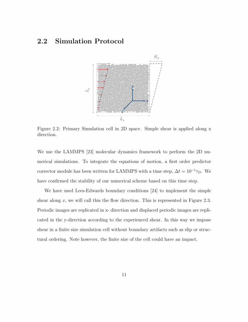
Figure 2.2: Primary Simulation cell in 2D space. Simple shear is applied along xdirection.

We use the LAMMPS [23] molecular dynamics framework to perform the 2D nu-

merical simulations. To integrate the equations of motion, a first order predictor

corrector module has been written for LAMMPS with a time step, ∆t = 10−1τD. We

have confirmed the stability of our numerical scheme based on this time step.

We have used Lees-Edwards boundary conditions [24] to implement the simple

shear along x, we will call this the flow direction. This is represented in Figure 2.3.

Periodic images are replicated in x- direction and displaced periodic images are repli-

cated in the y-direction according to the experienced shear. In this way we impose

shear in a finite size simulation cell without boundary artifacts such as slip or struc-

tural ordering. Note however, the finite size of the cell could have an impact.

11

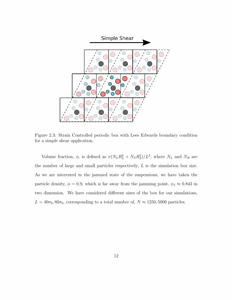
Figure 2.3: Strain Controlled periodic box with Lees Edwards boundary conditionfor a simple shear application.

Volume fraction, φ, is defined as π(NLR2L + NSR

2S)/L2, where NL and NR are

the number of large and small particles respectively, L is the simulation box size.

As we are interested in the jammed state of the suspensions, we have taken the

particle density, φ = 0.9, which is far away from the jamming point, φJ ≈ 0.843 in

two dimension. We have considered different sizes of the box for our simulations,

L = 40σ0, 80σ0, corresponding to a total number of, N ≈ 1250, 5000 particles.

12

Chapter 3

Rheology and Dissipated Energy

13

In the first part of this section, we describe the rheological behavior for the

overdamped bubble model; from the stress - strain response at very small deformation

rate to how it changes with increasing shearing rate. In the simple case of imposing

a constant linear shear rate γ on the system, the shear stress σxy may be obtained

from the usual microscopic Irving- Kirkwood definition [25], with m = 0,

σαβ =1

L2

N∑i=1

[1

2

N∑j=1,i=1

fijαrijβ −miviαvjβ

](3.1)

where α, β represent the Cartesian coordinates, ~rij = ~rj − ~ri, fij is the force exerted

by on j-th particle on i and vi is the velocity of i-th particle. We do not include the

contribution from viscous stress in the flow curves.

3.1 Rheology

By definition, ‘Rheology’ is the study of flow properties of liquids and soft mate-

rials under the condition where the response to applied stress is plastic in nature

instead of the well known elastic behavior of matter. For a linear elastic solid the

deformation is proportional to the applied stress in small deformation limit and is

governed by the Hooke's law, γ = G−1σ, where G is the shear modulus. Above

a certain value of stress, known as “yield stress” (σY ) the material deforms per-

manently due to plasticity. On the other hand, most of the familiar liquids follow

Newtonian behavior, σ ∝ γ; or in other words normal Newtonian liquids have a con-

stant viscosity η = σ/γ. But there are many other fluids like corn-starch in water,

paints, colloidal suspensions, which do not show constant viscosity and are classified

14

as non-Newtonian fluids.

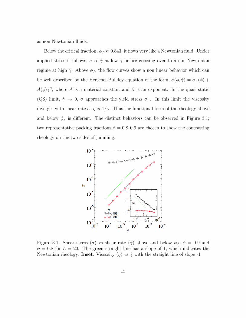
Below the critical fraction, φJ ≈ 0.843, it flows very like a Newtonian fluid. Under

applied stress it follows, σ ∝ γ at low γ before crossing over to a non-Newtonian

regime at high γ. Above φJ , the flow curves show a non linear behavior which can

be well described by the Herschel-Bulkley equation of the form, σ(φ, γ) = σY (φ) +

A(φ)γβ, where A is a material constant and β is an exponent. In the quasi-static

(QS) limit, γ → 0, σ approaches the yield stress σY . In this limit the viscosity

diverges with shear rate as η ∝ 1/γ. Thus the functional form of the rheology above

and below φJ is different. The distinct behaviors can be observed in Figure 3.1;

two representative packing fractions φ = 0.8, 0.9 are chosen to show the contrasting

rheology on the two sides of jamming.

Figure 3.1: Shear stress (σ) vs shear rate (γ) above and below φJ , φ = 0.9 andφ = 0.8 for L = 20. The green straight line has a slope of 1, which indicates theNewtonian rheology. Inset: Viscosity (η) vs γ with the straight line of slope -1

15

3.1.1 Stress vs Strain for Various Shearing Rate

0.25 0.3 0.35

0

0.001

0.002

γ

σxy

Figure 3.2: Macroscopic shear stress (σ) vs strain (γ) for γ = 10−7, very close to thequasi-static limit for L = 40.

When finite size samples of amorphous solids are driven slowly, the system spends

the majority of its time loading elastically with little dissipation and a minority of its

time undergoing large plastic dissipation. This behavior of bursty energy dissipation

during slow loading is seen in a many diverse systems including dislocation bursts in

crystal plasticity [26–29], domain wall motion in disordered magnets [30–32] and in

amorphous solids like our model [18, 19, 33–35]. In the QS limit, the events are well

separated from each other and occurs after a period of elastic loading. In Figure 3.2,

we have plotted the stress vs strain for a very slow shearing rate (γ = 10−7). Here,

one can clearly observe the stress drop due to distinct events which are followed by

several ramps of elastic loading [5, 20, 36].

16

1.15 1.2 1.25

10−3

10−2

!

" 8 ⇥ 10�5

8 ⇥ 10�3

8 ⇥ 10�7

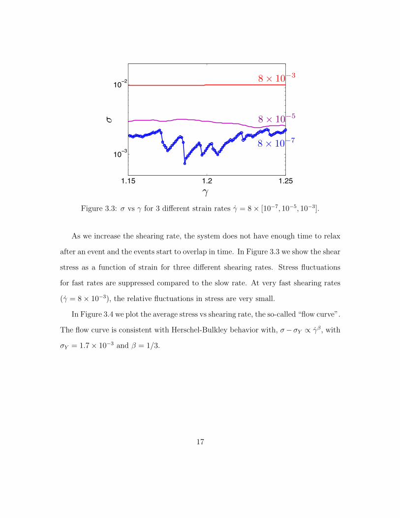
Figure 3.3: σ vs γ for 3 different strain rates γ = 8× [10−7, 10−5, 10−3].

As we increase the shearing rate, the system does not have enough time to relax

after an event and the events start to overlap in time. In Figure 3.3 we show the shear

stress as a function of strain for three different shearing rates. Stress fluctuations

for fast rates are suppressed compared to the slow rate. At very fast shearing rates

(γ = 8× 10−3), the relative fluctuations in stress are very small.

In Figure 3.4 we plot the average stress vs shearing rate, the so-called “flow curve”.

The flow curve is consistent with Herschel-Bulkley behavior with, σ−σY ∝ γβ, with

σY = 1.7× 10−3 and β = 1/3.

17

10−7

10−6

10−5

10−4

10−3

10−2

10−3

10−2

γ

σ

Figure 3.4: Flow stress (σ) vs strain rate (γ) for a jammed system(φ = 0.9), L = 40.The dashed line has a slope of 1/3.

(a) Dennin data (b) M. Van Hecke data

Figure 3.5: Experimental results for foams and bubbles from (a) Michael Dennin'sgroup [37] and (b) Martin Van Hecke's Group [10]. The black line in (a) has a slopeof 1/3 and the black curve in (b) is a Herschel Bulkley fit with an exponent of 0.35.

18

3.2 Instantaneous Energy Dissipation Rate

As we discussed above, in slowly driven disordered materials, energy dissipation is

expected to occur infrequently with a broad distribution of energy dissipation rates.

The energy dissipation rate, Q, can be expressed as the difference between the power

input due to the applied deformation, σγ 1, and time derivative of the total potential

energy dU/dt,

Q = σγ − dU

dt(3.2)

Time derivative of energy can be written as,

dU

dt=∂U

∂γ

∣∣∣∣s

γ +∑i

∂U

∂~si~si = σγ −

∑i

~Fi.δ~vi (3.3)

where, ~si is the position of the i-th particle in co-moving reference frame, δvi is the

non-affine velocity and ~Fi is the total force on particle i due to the harmonic springs

attached to it. ∂U∂γ

∣∣∣sγ can be identified as the applied work, σγ. Combining equations

3.2 and 3.3 we can get the expression for the instantaneous dissipation rate Q,

Q = Γγ =∑i

~Fi.δ~vi = b∑i

δv2i (3.4)

Γ being the energy dissipated per unit strain and b, the drag coefficient. It can be

noted that the total energy dissipated over all events occurring over a time interval

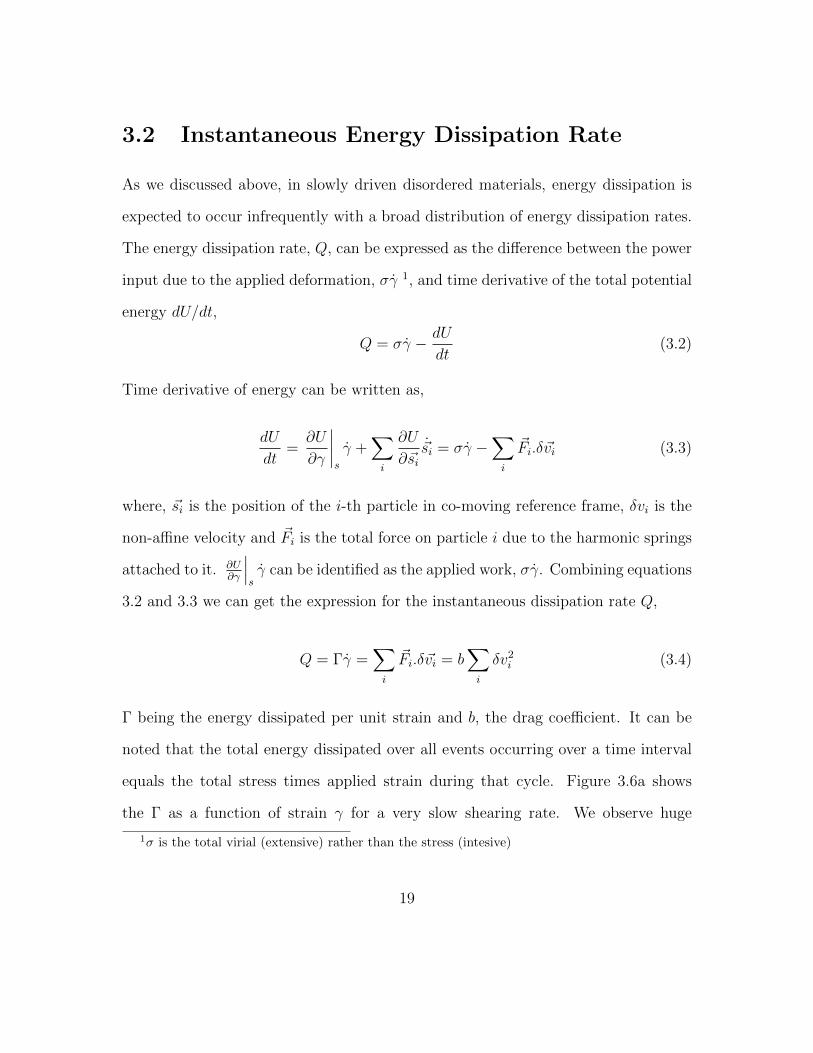
equals the total stress times applied strain during that cycle. Figure 3.6a shows

the Γ as a function of strain γ for a very slow shearing rate. We observe huge

1σ is the total virial (extensive) rather than the stress (intesive)

19

dissipation of energy at some particular instants which correspond to large, coherent

rearrangements. In Figure 3.6b, big spikes represent the plastic re-arrangements and

the small perturbations at small Γ corresponds to the regular response during the

elastic loading.

0.25 0.3 0.35

0

5

10

15

20

25

γ

Γ

(a) Linear scale

0.25 0.3 0.35

10−2

100

γ

Γ

(b) Semi-log scale

Figure 3.6: Instantaneous energy dissipated per unit strain (Γ) vs strain (γ) forγ = 10−7.

3.2.1 Quasistatic Scaling of Γ Distribution

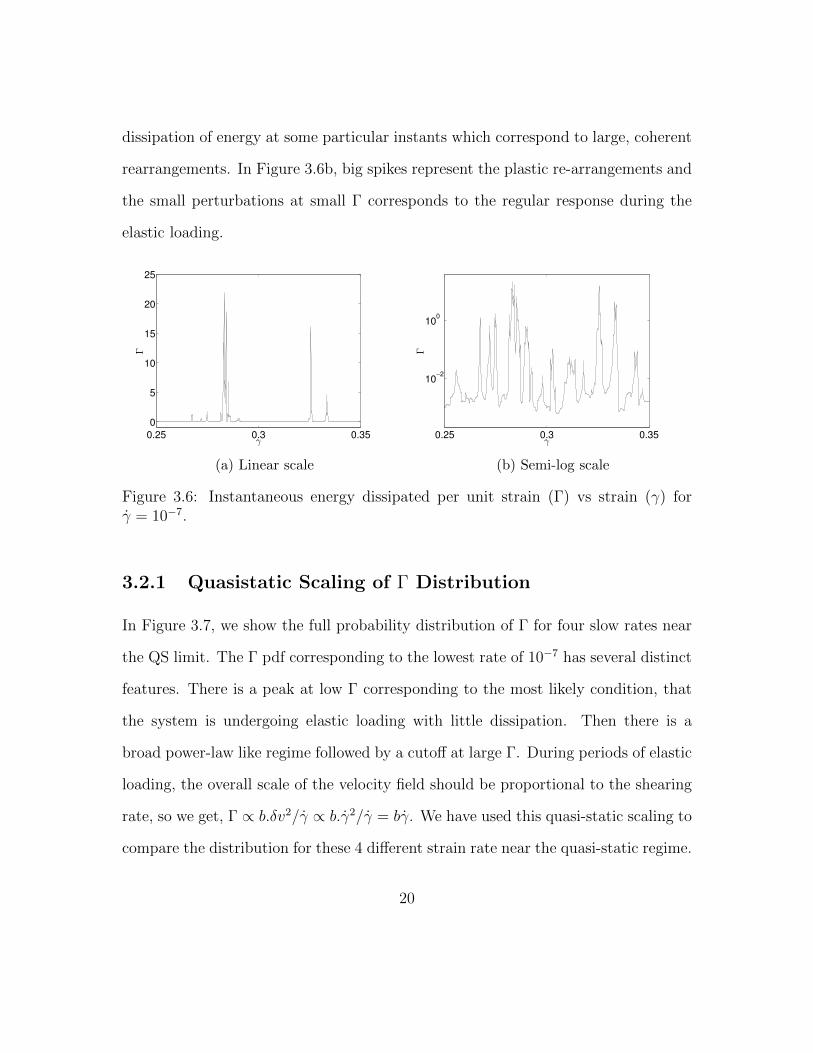
In Figure 3.7, we show the full probability distribution of Γ for four slow rates near

the QS limit. The Γ pdf corresponding to the lowest rate of 10−7 has several distinct

features. There is a peak at low Γ corresponding to the most likely condition, that

the system is undergoing elastic loading with little dissipation. Then there is a

broad power-law like regime followed by a cutoff at large Γ. During periods of elastic

loading, the overall scale of the velocity field should be proportional to the shearing

rate, so we get, Γ ∝ b.δv2/γ ∝ b.γ2/γ = bγ. We have used this quasi-static scaling to

compare the distribution for these 4 different strain rate near the quasi-static regime.

20

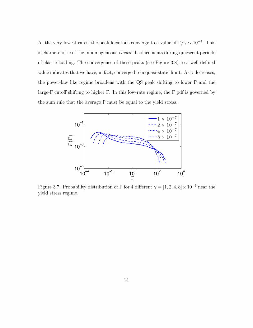
At the very lowest rates, the peak locations converge to a value of Γ/γ ∼ 10−4. This

is characteristic of the inhomogeneous elastic displacements during quiescent periods

of elastic loading. The convergence of these peaks (see Figure 3.8) to a well defined

value indicates that we have, in fact, converged to a quasi-static limit. As γ decreases,

the power-law like regime broadens with the QS peak shifting to lower Γ and the

large-Γ cutoff shifting to higher Γ. In this low-rate regime, the Γ pdf is governed by

the sum rule that the average Γ must be equal to the yield stress.

10−4

10−2

100

102

104

10−5

10−3

10−1

Γ

P(Γ

)

1 × 10−7

2 × 10−7

4 × 10−7

8 × 10−7

Figure 3.7: Probability distribution of Γ for 4 different γ = [1, 2, 4, 8]×10−7 near theyield stress regime.

21

102

104

106

108

1010

10−5

10−3

10−1

Γ/γ

P(Γ

)

1 × 10−7

2 × 10−7

4 × 10−7

8 × 10−7

Figure 3.8: Probability Distribution of Γ vs Γ scaled by rate for 4 different γ =[1, 2, 4, 8] × 10−7. The peaks corresponding to the elastic loading near the slow γlimit is clearly visible.

3.2.2 Strain Rate Dependence

1.15 1.2 1.25

10−2

100

102

!

!

8 ⇥ 10�5

8 ⇥ 10�3

8 ⇥ 10�7

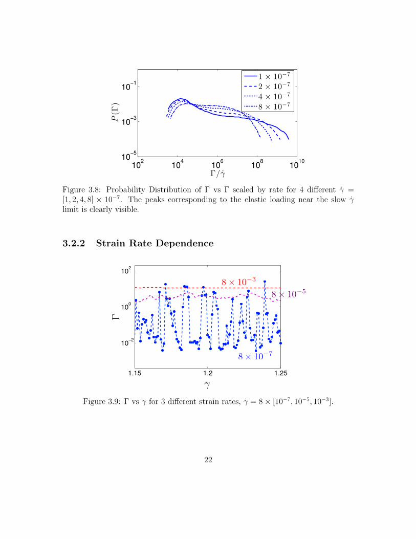
Figure 3.9: Γ vs γ for 3 different strain rates, γ = 8× [10−7, 10−5, 10−3].

22

With increasing strain rate γ, the motion becomes more uniform and the burstiness

in the system disappears. In Figure 3.9 we plot Γ vs strain (γ).The fluctuations

in Γ are minimized for faster rates (γ = 8 × 10−3). In Figure 3.10, we plot the Γ

PDFs of 20 different shearing rates (evenly spaced logarithmically). At low rates,

we see the broad power-law like distribution with QS peak at low Γ. At high rates,

the distributions are Gaussian. Recall that, 〈Γ〉 = 〈σ〉, so the flow curve completely

determines the position of the Gaussian peak at high rate.

10−2 100 10210−6

10−4

10−2

100

!

P(!

)

Figure 3.10: Probability distribution of Γ for a spectrum of strain rates, γ ∈ [1 ×10−7, 8× 10−3]. Blue curve denote slow γ, which is near QS regime and Red denotehigh γ where the system has no time for relaxation.

23

Chapter 4

Displacement Statistics

24

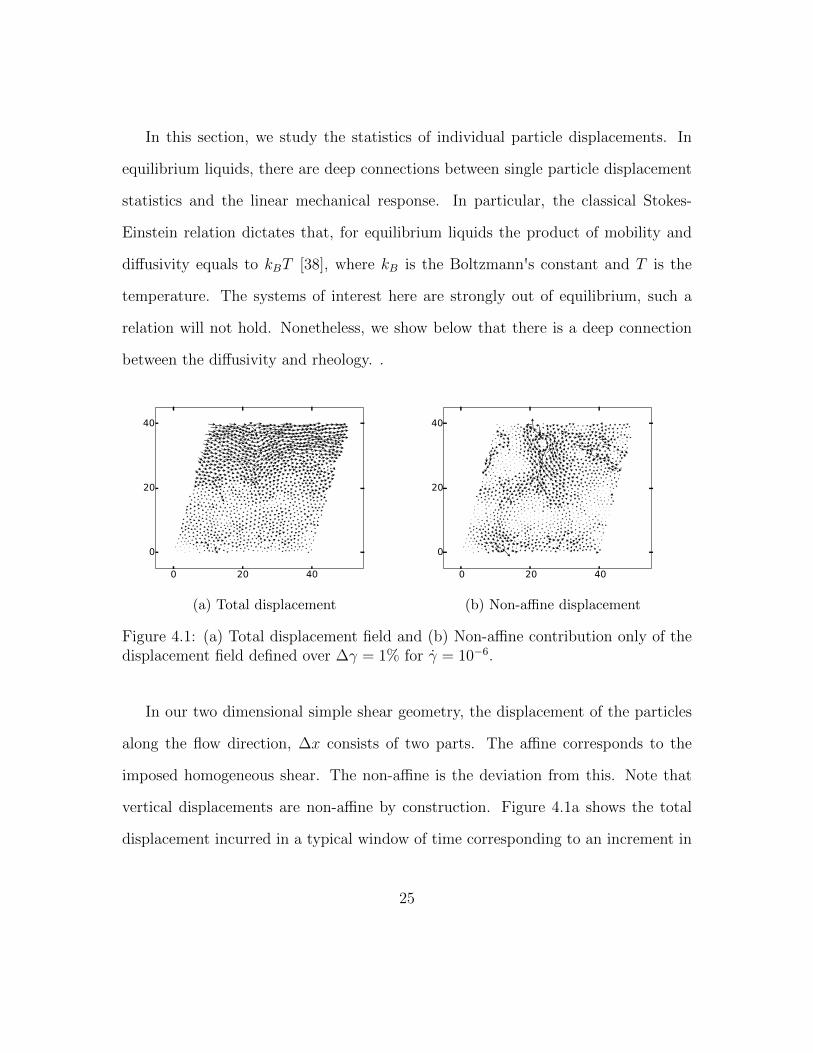
In this section, we study the statistics of individual particle displacements. In

equilibrium liquids, there are deep connections between single particle displacement

statistics and the linear mechanical response. In particular, the classical Stokes-

Einstein relation dictates that, for equilibrium liquids the product of mobility and

diffusivity equals to kBT [38], where kB is the Boltzmann's constant and T is the

temperature. The systems of interest here are strongly out of equilibrium, such a

relation will not hold. Nonetheless, we show below that there is a deep connection

between the diffusivity and rheology. .

0 20 40

0

20

40

(a) Total displacement

0 20 40

0

20

40

(b) Non-affine displacement

Figure 4.1: (a) Total displacement field and (b) Non-affine contribution only of thedisplacement field defined over ∆γ = 1% for γ = 10−6.

In our two dimensional simple shear geometry, the displacement of the particles

along the flow direction, ∆x consists of two parts. The affine corresponds to the

imposed homogeneous shear. The non-affine is the deviation from this. Note that

vertical displacements are non-affine by construction. Figure 4.1a shows the total

displacement incurred in a typical window of time corresponding to an increment in

25

shear strain of 1%. The displacements are dominated by the affine motion. In Figure

4.1b shows only the non-affine contribution.

4.1 Diffusive Behavior

If velocities eventually de-correlate, then the central limit theorem dictates that the

displacement distributions should tend to Gaussians with a variance that is linear in

time,

〈∆rα∆rβ〉 = 2Dαβ∆t (4.1)

where ∆rα is the displacement of a particle over ∆t in the α direction and Dαβ is the

self-diffusion constant. In the quasi-static regime applied strain plays the role of time

and particle rearrangements should depend only on the strain interval ∆γ. Based

on this argument we define an effective diffusion coefficient Dαβ = Dαβ/γ [39]. Here

we present the Mean Squared Displacement (MSD) as the square of the transverse

displacement 〈∆y2〉. We do this for simplicity, as the vertical displacements have

no contribution from the average flow. We would expect identical results for the

horizontal component once the appropriate background motion has been removed.

In Figure 4.2, the MSD for an intermediate strain rate (γ = 10−4) is plotted as

function of strain interval ∆γ. There exist two distinct regime, (a) Ballistic(at

small ∆γ) : ∆y ∝ ∆γ and (b) Diffusive(at large ∆γ) : ∆y2 ∝ ∆γ.

26

Figure 4.2: MSD in the transverse direction as a function of ∆γ for γ = 10−4, L = 20.Inset:〈∆y2〉/∆γ vs ∆γ. For large ∆γ, ∆y2/∆γ is constant.

In Figure 4.3, we plot the MSD vs ∆γ for a range of strain rates, γ ∈ [1×10−5, 8×

10−3]. For fast rates, MSD has a sharp crossover from the ballistic to diffusive regime.

For all rates, the velocities eventually decorrelate and the systems become diffusive.

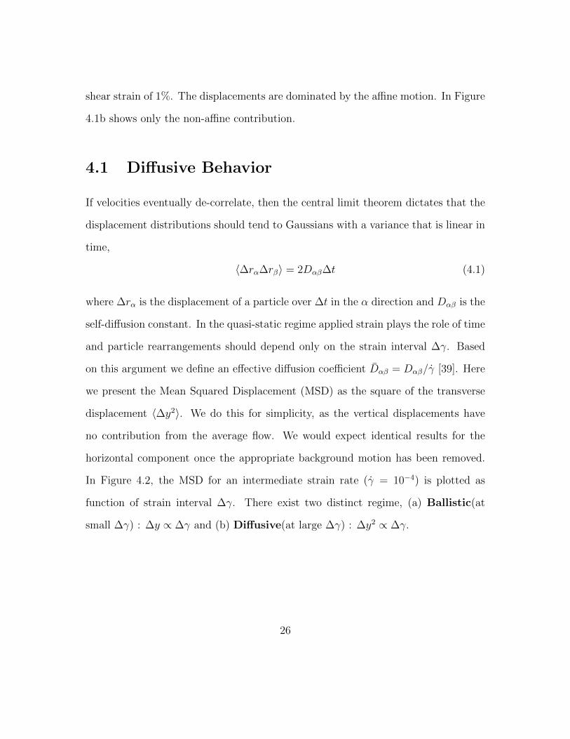
In Figure 4.5, we show the non-Gaussian parameter α = 3〈∆y2〉2/〈∆y4〉 for the

displacement distributions. For a Gaussian like distribution, α should be unity. For

relatively slower rates, ∆y distributions appear to be non-Gaussian at small ∆γ and

appear to reach the Fickian limit (both α = 1 and < ∆y2 >∝ ∆γ) at a much larger

∆γ ∼ 1. However, for fast rates ∆y distributions are always Gaussian and crosses

over to the Fickian limit at a similar ∆γ.

27

10−2 100 10210−2

10−1

100

!!

!!y2"/!!

!"

Increasing Rate

Diffusive

� 2 [1 ⇥ 10�05, 8 ⇥ 10�03]

Figure 4.3: Scaled second moment (〈∆y2〉/∆γ) vs strain window (∆γ) for differentrates, γ = [1, 2, 4, 8, 10, 20, 40, 80, 100, 200, 400, 800]× 10−5, L = 40. Red correspondto a fast rate (γ = 8 × 10−3) and violet correspond to a intermediate rate (γ =1× 10−5).

10−2

100

10−4

10−2

100

102

∆γ

〈∆y2〉/〈∆

γ〉

(a) 2nd moment

10−2

100

10−5

100

∆γ

〈∆y4〉/〈∆

γ〉2

(b) 4th moment

Figure 4.4: (a) Scaled second moment and (b) scaled fourth mo-ment of the displacement distribution for different rates, γ =[1, 2, 4, 8, 10, 20, 40, 80, 100, 200, 400, 800, 1000, 2000, 4000, 8000, 10000, 20000, 40000, 80000]×10−7, L = 40. Red correspond to a fast rate (γ = 8× 10−3) and blue correspond toa slow rate (γ = 1× 10−7).

28

10−2

100

10−2

10−1

100

101

∆γ

α

(a) 2nd moment

10−2

100

10−2

100

102

∆γ

γ2

(b) 4th moment

Figure 4.5: (a) Non-Gaussian parameter (α) and (b) kurtosis (γ2 =1/α − 1) of the displacement distribution for different rates, γ =[1, 2, 4, 8, 10, 20, 40, 80, 100, 200, 400, 800, 1000, 2000, 4000, 8000, 10000, 20000, 40000, 80000]×10−7, L = 40. Red correspond to a fast rate (γ = 8× 10−3) and blue correspond toa slow rate (γ = 1 × 10−7). The black dashed line in (a) corresponds to α = 1 andin (b) corresponds to γ2 ∝ 1/∆γ.

We define the effective diffusion coefficient (D) from the long time MSD for

different strain rate. In Figure 4.6, D is plotted as a function of rate, γ. D goes to

a plateau as we decrease γ, indicating that the long time dynamics does not depend

on the rate. This is the definition of quasi-static behavior. D starts to decrease

from the QS plateau at a crossover rate γ∗ ∼ 2 × 10−6. At high rate, D follows a

power law, D ∝ γ−1/3. The decrease in D also suggests that the long time spatial

correlation decreases as we shear the system rapidly.

29

10−7

10−6

10−5

10−4

10−3

10−2

10−1

100

γ

D

Figure 4.6: Effective Diffusion Coefficient (D) vs Strain rate (γ) for L = 40, φ = 0.9.The dashed line has a slope of -1/3.

In the QS limit, plastic rearrangements which occur during time intervals for

which the single-particle displacement statistics appear to be diffusive are expected

to organize into lines of slip, the so-called TSLs [3] (see schematic in Figure 4.7).

One can make a simple stochastic model for the effect of this organization on the

displacement of a typical particle. During each event, every particle gets a random

displacement, ∆y, chosen from a flat probability distribution, ∆y ∈ [−a/2, a/2]

where a is the displacement discontinuity in the TSL, assumed to be a constant. On

average, an event like this will induce a mean squared displacement, 〈∆y2〉TSL =

a2/12. Each event releases a strain of a/L, so they must occur once every ∆γTSL =

a/L on average to accommodate the imposed deformation. If subsequent TSLs are

spatially uncorrelated, one may invoke the central limit theorem to obtain:〈∆y2〉 =

NTSL〈∆y2〉TSL = ∆γ(L/a)(a2/12), whence:〈∆y2〉/∆γ = aL/12. For φ = 0.9, a =

(12/L)(2D) ∼ (12/40σ0)(2∗0.8σ20) ∼ 0.5σ0. D also provides an estimate of ∆γTSL =

30

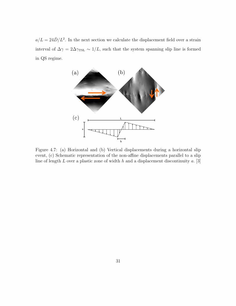
a/L = 24D/L2. In the next section we calculate the displacement field over a strain

interval of ∆γ = 2∆γTSL ∼ 1/L, such that the system spanning slip line is formed

in QS regime.

Figure 4.7: (a) Horizontal and (b) Vertical displacements during a horizontal slipevent, (c) Schematic representation of the non-affine displacements parallel to a slipline of length L over a plastic zone of width h and a displacement discontinuity a. [3]

31

Chapter 5

Spatial Correlations

32

In this section, we study spatial structure of the particle rearrangements. In the

first part, we briefly discuss the current understanding of plasticity in amorphous

materials and importance of studying spatial correlation of displacement and strain.

In the second part, we present the results obtained for the spatial structure of i) the

displacement field (defined over a particular interval of applied shear) and its spatial

gradient and ii) the instantaneous velocity field and its spatial gradient.

It is generally believed that deformation in amorphous materials is caused by the

accumulation of local, collective rearrangement of small number of particles [6, 40],

known as shear transformations or shear transformation zones [5,41]. Like dislocation

motion in a crystal, these shear transformations are the fundamental elementary

process allowing for plasticity in an amorphous solid. The idea of local flips or

shear transformations has been supported by numerical simulations [5,20,36,41,42].

Bulatov and Argon [43–45] were the first to point out that these rearrangements are

correlated in space and each rearrangement causes long-ranged strain fields [4,46–49],

which redistribute the stress in rest of the system.

5.1 The Eshelby Response

The Eshelby field corresponding to a single flip can be visualized as the far-field

response due to the two set of force dipoles (Figure 5.1a) acting at the origin in an

infinite, elastic medium [4]. The force F can be determined using the dipole strength

as F = 2aµ∆ε0, where µ is the shear modulus, a is the length scale over which the flip

occurs and ∆ε0 is the eigen strain at the core. Assuming the stress developed due to

33

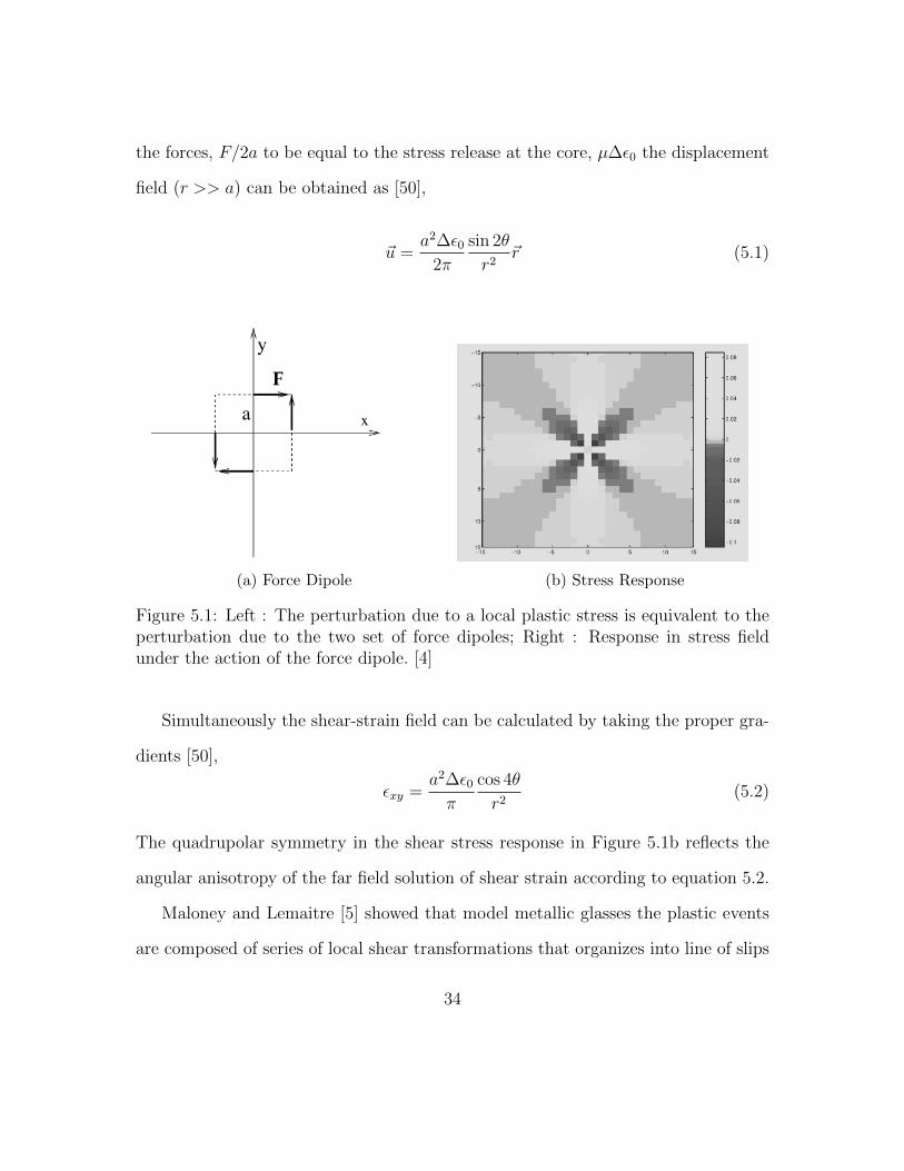
the forces, F/2a to be equal to the stress release at the core, µ∆ε0 the displacement

field (r >> a) can be obtained as [50],

~u =a2∆ε0

2π

sin 2θ

r2~r (5.1)

(a) Force Dipole (b) Stress Response

Figure 5.1: Left : The perturbation due to a local plastic stress is equivalent to theperturbation due to the two set of force dipoles; Right : Response in stress fieldunder the action of the force dipole. [4]

Simultaneously the shear-strain field can be calculated by taking the proper gra-

dients [50],

εxy =a2∆ε0π

cos 4θ

r2(5.2)

The quadrupolar symmetry in the shear stress response in Figure 5.1b reflects the

angular anisotropy of the far field solution of shear strain according to equation 5.2.

Maloney and Lemaitre [5] showed that model metallic glasses the plastic events

are composed of series of local shear transformations that organizes into line of slips

34

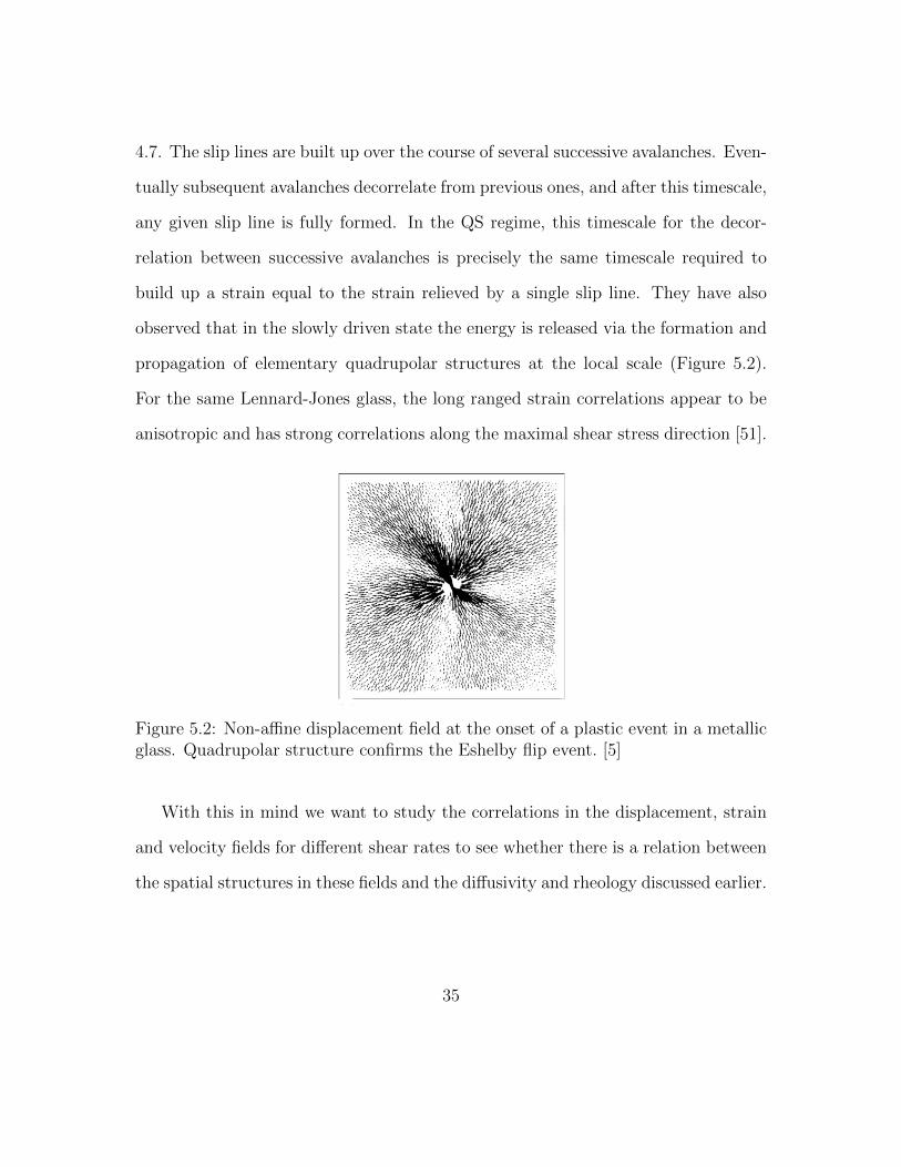
4.7. The slip lines are built up over the course of several successive avalanches. Even-

tually subsequent avalanches decorrelate from previous ones, and after this timescale,

any given slip line is fully formed. In the QS regime, this timescale for the decor-

relation between successive avalanches is precisely the same timescale required to

build up a strain equal to the strain relieved by a single slip line. They have also

observed that in the slowly driven state the energy is released via the formation and

propagation of elementary quadrupolar structures at the local scale (Figure 5.2).

For the same Lennard-Jones glass, the long ranged strain correlations appear to be

anisotropic and has strong correlations along the maximal shear stress direction [51].

Figure 5.2: Non-affine displacement field at the onset of a plastic event in a metallicglass. Quadrupolar structure confirms the Eshelby flip event. [5]

With this in mind we want to study the correlations in the displacement, strain

and velocity fields for different shear rates to see whether there is a relation between

the spatial structures in these fields and the diffusivity and rheology discussed earlier.

35

5.2 Displacement and Strain Correlation

We first calculate the displacement of each particle over a strain interval, ∆γ = 1/L.

In Lennard-Jones glasses Maloney et al. [3] showed that strain of 1/L is required to

create a transient slip line, that spans the whole system at quasi static limit. The

affine components arising due to the deformation of the box is subtracted off and

only the non-affine part is considered. The displacement field is then computed by

interpolating onto a regular mesh at the reference state. Figure 5.3 shows the typical

transverse displacement field (uy) for two different shear rate, γ = 8 × 10−7, 8 ×

10−3. Strong spatial correlations can be observed at slow shear rate regime and also

slip line like features are visible with a strong blue → red discontinuity indicating

a slip of roughly unit amplitude (∼ one small particle diameter). The slips are

aligned vertically, along the direction of maximum resolved shear at 45 degrees to

the principal stress axes (Figure 5.3a). On other hand, the correlations are very

short ranged when the system is sheared rapidly. The extent of special correlations

can be characterized by the correlation function of the respective displacement field.

36

(a) γ = 8× 10−7 (b) γ = 8× 10−3

Figure 5.3: Transverse displacement, ∆y, incurred between γ = 1.2 and γ = 1.225(∆γ = 0.025 ∼ 1/L) for (a) Slowly sheared system (γ = 8 × 10−7) and (b) Rapidlysheared system (γ = 8× 10−3). The displacement field is obtained by interpolatingthe particle displacements on a regular mesh-grid at the reference configuration whenγ = 1.2.

The spatial auto correlation function can be defined for any scalar field φ(~r) as,

Cφ(~R) = 〈φ(~r)φ(~r + ~R)〉~r (5.3)

Similarly in k-space the correlation is studied by the power spectrum and its

normalized version, structure factor,

Sφ(~k) =|φ(~k)|2Np

(5.4)

where, φ(~k) is the fourier space representation (see Appendix A) of φ(~r) and Np is

the normalization parameter.

In Figure5.4 we show both displacements uy and ux for a system of size L = 80. It

37

shows the real space correlation of the displacement components for a slow γ near the

diffusive plateau. We can see strong correlations along the longitudinal directions,

i.e, along x for Cux and along y for Cuy . These correspond to the vertically extended

features observed in Figure 5.3a and the corresponding horizontally extended features

in the horizontal displacements (not shown).

In Figure 5.5 and 5.6, we plot the value of the longitudinal and transverse real-

space correlations of the displacement field for various shearing rates. Figure 5.5a

shows the longitudinal correlations of the horizontal displacements (horizontal sepa-

ration); Figure 5.5b shows the transverse correlations of the horizontal displacement;

FIgure 5.6a shows the transverse correlations of the vertical displacement and Figure

5.6b shows the longitudinal correlations of the vertical displacement. With increas-

ing γ, the correlated behavior along the longitudinal direction decays faster which

is an evidence of decreasing correlation length, in agreement with the general im-

pression from Figure 5.3. Olsson and Teitel and co-workers [52,53] have studied the

instantaneous velocity correlation along the transverse direction near jamming and

showed that the correlation length diverges as a system nears the jamming transition.

For a jammed system (φ = 0.9), the displacement correlation along the transverse

direction has different behavior and functional form for different γ. For fast γ, it is

anti correlated after a few particle diameters and then decays to zero, whereas for

slow γ the correlation decays slowly and saturates at a negative value. In Figure 5.7,

we plot the correlation length ξ. We define ξ simply by the location of the minimum

in the correlation functions. Figure 5.7 shows that at low rate, ξ saturates near the

system size, while at higher rates, ξ scales like γ−1/3. At the very highest rates, ξ

38

saturates near the particle scale. At this point, there are essentially no longer any

spatial correlations in the system.

x

y

102× Cu x

−40 0 40−40

0

40

0

0.5

1

1.5

2

(a) Cux(~R)

xy

102× Cu y

−40 0 40−40

0

40

0

0.2

0.4

0.6

0.8

1

1.2

(b) Cuy(~R)

Figure 5.4: 2D spatial plot for correlation of displacement fields (ux and uy) forγ = 1× 10−7; Left: Cux and Right: Cuy . Displacements are calculated over a strainwindow of ∆γ ∼ 1/L.

10 20 30 40−0.2

0

0.2

0.4

0.6

0.8

1

x

Cux(x

)/C

ux(x

=1)

γ = 10−7

γ = 10−6

γ = 10−5

γ = 10−4

γ = 10−3

(a) Cux vs x

10 20 30 40−0.4

−0.2

0

0.2

0.4

0.6

0.8

1

y

Cux(y

)/C

ux(y

=1)

γ = 10−7

γ = 10−6

γ = 10−5

γ = 10−4

γ = 10−3

(b) Cux vs y

Figure 5.5: Correlation of x-displacement along x (Left) and along y (Right) fordifferent strain rates (γ = 10−3, 10−4, 10−5, 10−6, 10−7). The red dashed lines arezero correlation.

39

10 20 30 40−0.4

−0.2

−0

0.2

0.4

0.6

0.8

1

x

Cuy(x

)/C

uy(x

=1)

γ = 10−7

γ = 10−6

γ = 10−5

γ = 10−4

γ = 10−3

(a) Cuy vs x

10 20 30 40−0.2

0

0.2

0.4

0.6

0.8

1

y

Cuy(y

)/C

uy(y

=1)

γ = 10−7

γ = 10−6

γ = 10−5

γ = 10−4

γ = 10−3

(b) Cuy vs y

Figure 5.6: Correlation of y-displacement along x (Left) and along y (Right) fordifferent strain rates (γ = 10−3, 10−4, 10−5, 10−6, 10−7). The red dashed lines arezero correlation.

10−8

10−6

10−4

10−2

100

101

102

γ

ξL

Figure 5.7: Correlation length (ξ) vs strain rate (γ) for L = 80. The red dashed linehas a slope of -1/3.

In Figure 5.8 we plot the power spectrum of ux and uy for low shear rate (1×10−7).

We observe similar patterns for both ux and uy; the patterns look to be rotated

40

by π/2. In Figure 5.9, we plot the power of vertical and horizontal displacements

along vertical and horizontal wavevectors at various shearing rate. With increasing

γ there is a development of peak whose location shifts to the right along k. This

rate dependence of transverse power is analogous to the transverse correlation in real

space. One can read a correlation length, (ξ), similar to the real space based on the

location of the maximum in transverse power. The location of peak power scales like

k∗ ∼ γ1/3. It is surprising to see that the longitudinal power is so insensitive to γ

compare to the transverse power.

kx/2π

ky/2π

log10(Su y)

−1 0 1−1

0

1

−2

−1

0

1

2

3

(a) Sux

kx/2π

ky/2π

log10(Sux)

−1 0 1−1

0

1

−2

−1

0

1

2

3

(b) Suy

Figure 5.8: Power of x-displacement (Left) and y-displacement (Right) for γ =1 × 10−7 and displacement calculated over a strain interval of ∆γ ∼ 1/L; Left: Suxand Right: Suy . A logarithmic(base10) color scale is used to show the magnitude.

41

10−2

10−1

100

101

102

103

104

105

kx/2π

Sux/Sux(k

x=

π)

γ = 10−7

γ = 10−6

γ = 10−5

γ = 10−4

γ = 10−3

(a) Sux vs kx

10−2

10−1

100

101

102

103

104

105

ky/2π

Sux/Sux(k

y=

π)

γ = 10−7

γ = 10−6

γ = 10−5

γ = 10−4

γ = 10−3

(b) Sux vs ky

10−2

10−1

100

101

102

103

104

105

kx/2π

Suy/Suy(k

x=

π)

γ = 10−7

γ = 10−6

γ = 10−5

γ = 10−4

γ = 10−3

(c) Suy vs kx

10−2

10−1

100

101

102

103

104

105

ky/2π

Suy/Suy(k

y=

π)

γ = 10−7

γ = 10−6

γ = 10−5

γ = 10−4

γ = 10−3

(d) Suy vs ky

Figure 5.9: Power of x-displacement along kx (a) and along ky (b), power ofy-displacement along kx (c) and along ky (d) for different strain rates (γ =10−3, 10−4, 10−5, 10−6, 10−7). The red dashed lines in (a),(d) have slopes of -1.5 andin (b),(c) have slopes of -2.5 respectively. The transverse power is more sensitive to γthan the longitudinal power of the displacement field. In the transverse power thereis a peak at increasing k with increasing γ indicating a decaying correlation lengthwith increasing γ.

42

We also compute gradients of the displacements (strains) and their correlations.

Displacement gradients ∂xux, ∂yux, ∂xuy, ∂yuy

Symmetric strain (∂yux + ∂xuy)/2

Vorticity (∂yux − ∂xuy)/2

The components of the strain tensor are obtained by taking the numerical gradients

on our interpolated displacement field. In Figure 5.10 and 5.11 we show 2D images

of real space correlation in the displacement gradients and the power spectrum re-

spectively. Although the x-gradient of ux is much smaller than the y-gradient, we

can see a four-fold symmetry in the correlation of ∂xux. This tells us that during

the plastic events the compacting region is always at an angle of π/4 with the region

that is dilating. Instead of studying the individual components of the strain tensor,

the symmetric strain (ε) and vorticity (ω) are commonly used as the measure for

plastic deformation [48, 51]. In Figure 5.12 we show the correlation in ε and ω field

for γ = 10−7. Strong positive correlations can be observed along the x and y direc-

tions. A quadrupolar structure similar to the Eshelby response can also be seen in

the strain correlation. Other researchers [4, 48, 51] have argued that for amorphous

materials, the elastic strain around a localized plastic zone decays with the distance

(r) with a power law. In Figure 5.13 we plot the ε correlation function in real space

along the horizontal direction for various rate. It decays like r−1 with a sharp cutoff.

The cutoff is consistent with the γ−1/3 scaling but we have not performed a precise

determination of it. Cε has a cutoff which goes to shorter length as γ increases, con-

sistent with the cutoff on the displacement correlations. In Figure 5.14 we show the

power of strain and vorticity field for a slowly sheared system (γ = 10−7). Prominent

43

quadrupolar symmetry along kx and ky is observed in the strain power spectrum. In

Figure 5.15, we show, Sε ∝ k−2/3x .

x

y

103× C∂xu x

−40 0 40−40

0

40

−0.05

0

0.05

(a) C∂xux

xy

103× C∂ yu x

−40 0 40−40

0

40

−0.5

0

0.5

(b) S∂yux

x

y

103× C∂xu y

−40 0 40−40

0

40

−0.5

0

0.5

(c) C∂xuy

x

y

103× C∂ yu y

−40 0 40−40

0

40

−0.05

0

0.05

(d) C∂yuy

Figure 5.10: Correlation of gradients of x and y-displacement for γ = 1× 10−7; (a):C∂xux , (b): C∂yux , (c): C∂xuy , (d): C∂yuy .

44

kx/2π

ky/2π

log10(S∂xux)

−1 0 1−1

0

1

−1.5

−1

−0.5

0

0.5

(a) S∂xux

kx/2π

ky/2π

log10(S∂yux)

−1 0 1−1

0

1

−1

−0.5

0

0.5

1

(b) S∂yux

kx/2π

ky/2π

log10(S∂xu y)

−1 0 1−1

0

1

−1

−0.5

0

0.5

1

(c) S∂xuy

kx/2π

ky/2π

log10(S∂yu y)

−1 0 1−1

0

1

−1.5

−1

−0.5

0

0.5

(d) S∂yuy

Figure 5.11: Structure factor of gradients of x and y-displacement for γ = 1× 10−7;(a): S∂xux , (b): S∂yux , (c): S∂xuy , (d): S∂yuy . A logarithmic(base10) color scale isused to show the magnitude.

45

x

y10

3× Cǫ

−40 0 40−40

0

40

−0.05

0

0.05

0.1

(a) Cε

x

y

103× Cω

−40 0 40−40

0

40

0

0.01

0.02

0.03

0.04

0.05

(b) Cω

Figure 5.12: Symmetric strain and vorticity correlation for γ = 1× 10−7; Right: Cεand Left: Cω. The quadrupolar symmetry in strain and vorticity is similar to theEshelby response for a force dipole at the origin.

100

101

102

10−3

10−2

10−1

100

101

x

Cǫ(x

)/C

ǫ(x

=1)

γ = 10−7

γ = 10−6

γ = 10−5

γ = 10−4

γ = 10−3

Figure 5.13: Normalized Cε vs x for L = 80, ∆γ = 1%, γ =10−3, 10−4, 10−5, 10−6, 10−7. The dashed red line has a slope of -1.

46

kx/2π

ky/2π

log10(Sǫ)

−1 0 1−1

0

1

−1

−0.5

0

0.5

(a) Sε

kx/2π

ky/2π

log10(Sω)

−1 0 1−1

0

1

−1

−0.5

0

0.5

(b) Sω

Figure 5.14: Structure factor of strain (Sε) vorticity (Sω) for γ = 1× 10−7; Left: Sεand Right: Sω. A logarithmic(base10) color scale is used to show the magnitude.

10−2

10−1

10−1

100

101

102

103

kx/2π

Sǫ/Sǫ(k

x=

π)

γ = 10−7

γ = 10−6

γ = 10−5

γ = 10−4

γ = 10−3

Figure 5.15: Power of strain (Sε) along kx, for γ = 1× [10−7, 10−6, 10−5, 10−4, 10−3].The red dashed line has a slope of -2/3

47

5.3 Velocity and Strain-rate Correlation

Previously, Ono. et al. [54] studied the velocity distributions “in this model” for

different strain rates (γ). They reported that the width of the distribution increased

sub-linearly with increasing γ. They argued that above a characteristic strain rate

(γ∗), the velocity distribution becomes Gaussian, correlations show exponential be-

havior in space and time and below γ∗ the distribution is broader than Gaussian

with correlations decaying as a stretched exponential. Here we want to study the

spatial structure of the instantaneous velocity and how it is related to the long time

displacement correlation. In Figure 5.16 we show the transverse particle velocities

during and after a plastic event (when Γ and dσ/dt are large) has occurred for a slow

rate (γ = 10−7). During the event the velocity field shows a line of slip. After the

completion of the event the velocity field is essentially uniform.

In Figure 5.17, we show a typical velocity field at some instant for a system

sheared at faster rate (γ = 10−3). At this rate, the stress is well above the yield

stress. As we showed above, the behavior is smooth in time. The dissipation rate

has very small relative fluctuations. Statistically, any instant is like any other. Quite

surprisingly, despite the smoothness in time, we continue to see spatially extended

structures. The image is dominated by a single, strong, vertical slip line with particle

velocities equal to about 2×10−3. Extended structures like these move smoothly and

continuously through the system over time and exhibit none of the burst behavior

observed at low rate near the yield stress.

In Figure5.18, we show the real-space correlation of the vertical velocities at two

different rates, one fast (γ = 10−3) and one slow (γ = 10−7). They both show

48

extended features along the vertical direction characteristic of the slip lines apparent

in Figure 5.16a and Figure 5.17. In Figure 5.19, in analogy with our analysis for

the finite-time displacement fields, we plot the correlation along the vertical and

horizontal directions for vertical velocity and do the same for the horizontal velocity

correlations.

Our data for the velocity correlations along the transverse directions (Figure

5.19b,c) have similar trend as Olsson and Teitel and co-workers [52, 53] found near

jamming (φ → φJ), although our system is highly jammed (φ = 0.9). In Figure

5.20, we plot the correlation length, ξ′ based on the location of the minimum in Cvy

along x direction. ξ′ obeys a power law, ξ′ ∝ γ−1/3, similar to ξ (correlation length

observed for displacement).

(a) Active state (b) Quiescent state

Figure 5.16: The y-velocity (vy) of particles before an event (Left) and after theevent has occurred (Right) are plotted for a slow rate (γ = 8× 10−7).

49

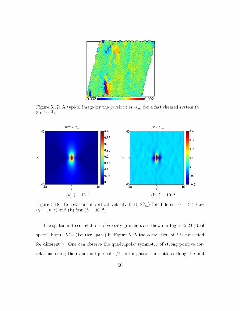
Figure 5.17: A typical image for the y-velocities (vy) for a fast sheared system (γ =8× 10−3).

x

y

1010× Cvy

−40 0 40−40

0

40

0

0.05

0.1

0.15

0.2

0.25

0.3

0.35

0.4

(a) γ = 10−7x

y

106× Cu y

−40 0 40−40

0

40

−0.2

−0.1

0

0.1

0.2

0.3

0.4

(b) γ = 10−3

Figure 5.18: Correlation of vertical velocity field (Cvy) for different γ : (a) slow(γ = 10−7) and (b) fast (γ = 10−3).

The spatial auto correlations of velocity gradients are shown in Figure 5.23 (Real

space) Figure 5.24 (Fourier space).In Figure 5.25 the correlation of ε is presented

for different γ. One can observe the quadrupolar symmetry of strong positive cor-

relations along the even multiples of π/4 and negative correlations along the odd

50

multiples of π/4, for both rates γ = 10−7 and 10−3. In Figure 5.26, we plot the real

space shear strain rate correlations along the horizontal (maximum shear) direction.

The correlations decay as roughly r−2 up to a rate dependent cutoff, consistent with

the velocity power spectra and the Eshelby solution.

10 20 30 40−0.2

0

0.2

0.4

0.6

0.8

1

x

Cvx(x

)/C

vx(x

=1)

γ = 10−7

γ = 10−6

γ = 10−5

γ = 10−4

γ = 10−3

(a) Cvx vs x

10 20 30 40−0.4

−0.2

0

0.2

0.4

0.6

0.8

1

y

Cvx(y

)/C

vx(y

=1)

γ = 10−7

γ = 10−6

γ = 10−5

γ = 10−4

γ = 10−3

(b) Cvx vs y

10 20 30 40−0.4

−0.2

0

0.2

0.4

0.6

0.8

1

x

Cvy(x

)/C

vy(x

=1)

γ = 10−7

γ = 10−6

γ = 10−5

γ = 10−4

γ = 10−3

(c) Cvy vs x

10 20 30 40−0.2

0

0.2

0.4

0.6

0.8

1

y

Cvy(y

)/C

vy(y

=1)

γ = 10−7

γ = 10−6

γ = 10−5

γ = 10−4

γ = 10−3

(d) Cvy vs y

Figure 5.19: Correlation of x velocity along x (a) and along y (b); Correla-tion of y velocity along x (c) and along y (d) for different strain rates (γ =10−3, 10−4, 10−5, 10−6, 10−7). The red dashed lines are guide for zero correlation.

51

Figure 5.20: Correlation length vs strain rate for L = 80. The red dashed line hasa slope of -1/3. ξ′ is calculated by taking the minimum of the correlation functionsplotted in Figure 5.19c.

kx/2π

ky/2π

log10(Svx)

−1 0 1−1

0

1

−2

−1.5

−1

−0.5

0

0.5

1

1.5

2

(a) Svx

kx/2π

ky/2π

log10(Svy)

−1 0 1−1

0

1

−2

−1.5

−1

−0.5

0

0.5

1

1.5

2

(b) Svy

Figure 5.21: Power spectrum of x-velocity (Left) and y-velocity (Right) for γ =1× 10−7. A logarithmic(base10) color scale is used to show the magnitude.

52

10−2

10−1

100

101

102

103

104

105

kx/2π

Svx/Svx(k

x=

π)

γ = 10−7

γ = 10−6

γ = 10−5

γ = 10−4

γ = 10−3

(a) Svx vs kx

10−2

10−1

100

101

102

103

104

105

ky/2π

Svx/Svx(k

y=

π)

γ = 10−7

γ = 10−6

γ = 10−5

γ = 10−4

γ = 10−3

(b) Svx vs ky

10−2

10−1

100

101

102

103

104

105

kx/2π

Svy/Svy(k

x=

π)

γ = 10−7

γ = 10−6

γ = 10−5

γ = 10−4

γ = 10−3

(c) Svy vs kx

10−2

10−1

100

101

102

103

104

105

ky/2π

Svy/Svy(k

y=

π)

γ = 10−7

γ = 10−6

γ = 10−5

γ = 10−4

γ = 10−3

(d) Svy vs ky

Figure 5.22: Power of x-velocity along kx (a) and along ky (b), power ofy-velocity along kx (c) and along ky (d) for different strain rates (γ =10−3, 10−4, 10−5, 10−6, 10−7). The red dashed lines have slopes of -2.

53

x

y10

12× C∂xvx

−40 0 40−40

0

40

−0.6

−0.4

−0.2

0

0.2

0.4

0.6

(a) C∂xvx

x

y

1012× C∂ yvx

−40 0 40−40

0

40

−5

0

5

(b) S∂yvx

x

y

1012× C∂xvy

−40 0 40−40

0

40

−5

0

5

(c) C∂xvy

x

y

1012× C∂ yvy

−40 0 40−40

0

40

−0.6

−0.4

−0.2

0

0.2

0.4

0.6

(d) C∂yvy

Figure 5.23: Correlation of gradients of x and y-velocities for γ = 1 × 10−7; (a):C∂xvx , (b): C∂yvx , (c): C∂xvy , (d): C∂yvy .

54

kx/2π

ky/2π

log10(S∂xvx)

−1 0 1−1

0

1

−1.5

−1

−0.5

0

0.5

(a) S∂xvx

kx/2π

ky/2π

log10(S∂yvx)

−1 0 1−1

0

1

−1.5

−1

−0.5

0

0.5

1

1.5

(b) S∂yvx

kx/2π

ky/2π

log10(S∂xvy)

−1 0 1−1

0

1

−1.5

−1

−0.5

0

0.5

1

1.5

(c) S∂xvy

kx/2π

ky/2π

log10(S∂yvy)

−1 0 1−1

0

1

−1.5

−1

−0.5

0

0.5

(d) S∂yvy

Figure 5.24: Power spectrum of gradients of x and y-velocities for γ = 1× 10−7; (a):S∂xvx , (b): S∂yvx , (c): S∂xvy , (d): S∂yvy . A logarithmic(base10) color scale is used toshow the magnitude.

55

x

y10

12× C ǫ

−40 0 40−40

0

40

−1

−0.5

0

0.5

1

(a) γ = 10−7x

y

107× C ǫ

−40 0 40−40

0

40

−0.5

−0.25

0

0.25

0.5

(b) γ = 10−3

Figure 5.25: Correlation of symmetric strain-rate (Cε) for γ = 1 × 10−7 in (a) andγ = 1× 10−3 in (b).

100

101

102

10−4

10−3

10−2

10−1

100

101

x

Cǫ(x

)/C

ǫ(x

=1)

γ = 10−7

γ = 10−6

γ = 10−5

γ = 10−4

γ = 10−3

Figure 5.26: Normalized Cε vs x for L = 80, γ = 10−3, 10−4, 10−5, 10−6, 10−7. Thedashed red line has a slope of -2.

56

Chapter 6

Summary and Future Work

57

We have performed numerical simulations to study the behavior of soft particle

jammed suspensions under simple shear. In order to study the interparticle interac-

tions under the flow, we have used the mean field version of Durian bubble model [22]

where the repulsive forces due to the contact deformation of the soft particles are

balanced by the viscous force caused by the background shear flow. The model

shows yield stress behavior (σ − σY ∝ γβ) above jamming (φ > φJ), similar to the

experiments on foams and soft suspensions [1, 10, 10, 37]. We have found avalanche

statistics near the yield stress plateau (vanishing rates, low γ) and uniform, Gaus-

sian probability distribution of Γ (Energy dissipated per unit strain) for high γ. The

results are consistent with the idea of having discrete, individual plastic events at

the quasistatic shear and overlapping nature of small events at fast rate.

To characterize the particle motion at different γ, we have studied Mean Squared

Displacement (MSD) and identified the diffusive motion irrespective of γ for large

strain intervals. For high γ, the particles move in a super-diffusive (∆y ∝ ∆γ)

manner at short strain, before undergoing a crossover to diffusive motion (∆y2 ∝ ∆γ)

at large strain. The long time effective diffusion coefficient (D = D/γ) saturates at

a rate independent value near the quasistatic regime. This can be understood by

the irreversible motion of the particles that go through the plastic rearrangements.

With increasing γ, D decreases following a power law, D ∝ γ−1/3. This reflects the

fact that the distance moved per unit strain decreases with increasing shear rate.

We have studied the displacement fields and its spatial correlations in Chapter

5. Correlation in displacement field grows with decreasing γ and saturates at the

system size at vanishing rates. The corresponding correlation length shows a power

58

law dependence on strain rate, ξ ∝ γ−1/3, similar to D. We have also observed a long

ranged quadrupolar symmetry in strain-strain correlation (Cε) which indicates that

the plastic deformation is caused by the accumulation of several Eshelby flips [4].

To connect the long time plasticity with the instantaneous propagation of stress we

have studied the spatial correlations of velocity field and its gradients. It was very

surprising to find a four-fold symmetry even in the strain-rate (ε) spatial autocorre-

lation, Cε ∝ cos(4θ)/r2. However the extent of power law decay is more severe in Cε

(∝ r−2) than the Cε (∝ r−1) along the strong correlation direction.

10−5

100

10−4

10−3

10−2

10−1

γτD

σxy

0.0625

0.25

1

4

16

64

∼ γ1/2

Figure 6.1: Stress vs strain rate for different damping constant for the Pair-Dragmodel.

Currently, we are trying to understand the spatial structures of these amorphous

materials considering a more sophisticated damping mechanism (Pair Drag model),

where the drag is proportional to relative velocities of the interacting particles. We

have already observed that in this pair drag model, the rheology (see Figure 6.1) and

diffusive properties matches the behavior of non-inertial bubble model qualitatively

59

with different power law exponents. In the overdamped limit, the flow curve follows,

σ− σY ∝ γ1/2 and effective diffusion obeys, D ∝ γ−1/2 for finite rates away from the

yield stress plateau. In the remaining period of my graduate studies, I also want to

relate the diffusion characteristics to the flow rheology based on the inferred results

from spatial correlations for these simple bubble models.

60

Bibliography

[1] K. N. Nordstrom, E. Verneuil, P. E. Arratia, a. Basu, Z. Zhang, a. G. Yodh,J. P. Gollub, and D. J. Durian, “Microfluidic Rheology of Soft Colloids aboveand below Jamming,” Phys. Rev. Lett., vol. 105, p. 175701, Oct. 2010.

[2] J. R. Seth, L. Mohan, C. Locatelli-Champagne, M. Cloitre, and R. T. Bonnecaze,“A micromechanical model to predict the flow of soft particle glasses.,” Nat.Mater., vol. 10, pp. 838–43, Nov. 2011.

[3] C. E. Maloney and M. O. Robbins, “Evolution of displacements and strains insheared amorphous solids,” J. Phys. Condens. Matter, vol. 20, p. 244128, June2008.

[4] G. Picard, a. Ajdari, F. Lequeux, and L. Bocquet, “Elastic consequences of asingle plastic event: a step towards the microscopic modeling of the flow of yieldstress fluids.,” Eur. Phys. J. E. Soft Matter, vol. 15, pp. 371–81, Dec. 2004.

[5] C. E. Maloney and A. Lemaıtre, “Amorphous systems in athermal, quasistaticshear.,” Phys. Rev. E. Stat. Nonlin. Soft Matter Phys., vol. 74, p. 016118, July2006.

[6] J.-L. Barrat and A. Lemaıtre, “Heterogeneities in amorphous systems undershear,” Dynamical Heterogeneities in Glasses, Colloids, and Granular Media,vol. 150, p. 264, 2011.

[7] G. Katgert, A. Latka, M. E. Mobius, and M. van Hecke, “Flow in linearlysheared two-dimensional foams: From bubble to bulk scale,” Physical ReviewE, vol. 79, no. 6, p. 066318, 2009.

[8] G. Katgert, M. Mobius, and M. van Hecke, “Rate Dependence and Role of Dis-order in Linearly Sheared Two-Dimensional Foams,” Phys. Rev. Lett., vol. 101,p. 058301, July 2008.

61

[9] G. Katgert, B. P. Tighe, M. E. Mobius, and M. van Hecke, “Couette flow oftwo-dimensional foams,” EPL (Europhysics Letters), vol. 90, no. 5, p. 54002,2010.

[10] M. E. Mobius, G. Katgert, and M. van Hecke, “Relaxation and flow in linearlysheared two-dimensional foams,” EPL (Europhysics Lett.), vol. 90, p. 44003,May 2010.

[11] V. Chikkadi, G. Wegdam, D. Bonn, B. Nienhuis, and P. Schall, “Long-RangeStrain Correlations in Sheared Colloidal Glasses,” Phys. Rev. Lett., vol. 107,p. 198303, Nov. 2011.

[12] L. Mohan, M. Cloitre, and R. T. Bonnecaze, “Active microrheology of softparticle glasses,” J. Rheol. (N. Y. N. Y)., vol. 58, pp. 1465–1482, Sept. 2014.

[13] A. Basu, Y. Xu, T. Still, P. E. Arratia, Z. Zhang, K. N. Nordstrom, J. M. Rieser,J. P. Gollub, D. J. Durian, and a. G. Yodh, “Rheology of soft colloids across theonset of rigidity: scaling behavior, thermal, and non-thermal responses.,” SoftMatter, vol. 10, pp. 3027–35, May 2014.

[14] L. Mohan, C. Pellet, M. Cloitre, and R. Bonnecaze, “Local mobility and mi-crostructure in periodically sheared soft particle glasses and their connection tomacroscopic rheology,” J. Rheol. (N. Y. N. Y)., vol. 57, no. 3, p. 1023, 2013.

[15] L. Mohan, R. T. Bonnecaze, and M. Cloitre, “Microscopic Origin of Inter-nal Stresses in Jammed Soft Particle Suspensions,” Phys. Rev. Lett., vol. 111,p. 268301, Dec. 2013.

[16] B. P. Tighe, E. Woldhuis, J. J. Remmers, W. van Saarloos, and M. van Hecke,“Model for the scaling of stresses and fluctuations in flows near jamming,” Phys-ical review letters, vol. 105, no. 8, p. 088303, 2010.

[17] C. P. Goodrich, S. Dagois-Bohy, B. P. Tighe, M. van Hecke, A. J. Liu, andS. R. Nagel, “Jamming in finite systems: Stability, anisotropy, fluctuations, andscaling,” Phys. Rev. E, vol. 90, p. 022138, Aug 2014.

[18] S. Tewari, D. Schiemann, D. J. Durian, C. M. Knobler, S. a. Langer, and a. J.Liu, “Statistics of shear-induced rearrangements in a two-dimensional modelfoam.,” Phys. Rev. E. Stat. Phys. Plasmas. Fluids. Relat. Interdiscip. Topics,vol. 60, no. 4 Pt B, pp. 4385–4396, 1999.

62

[19] K. Salerno, C. Maloney, and M. Robbins, “Avalanches in Strained AmorphousSolids: Does Inertia Destroy Critical Behavior?,” Phys. Rev. Lett., vol. 109,p. 105703, Sept. 2012.

[20] C. Maloney and A. Lemaıtre, “Subextensive Scaling in the Athermal, Qua-sistatic Limit of Amorphous Matter in Plastic Shear Flow,” Phys. Rev. Lett.,vol. 93, p. 016001, July 2004.

[21] C. S. O’Hern, L. E. Silbert, and S. R. Nagel, “Jamming at zero temperature andzero applied stress: The epitome of disorder,” Phys. Rev. E, vol. 68, p. 011306,July 2003.

[22] D. J. Durian, “Foam Mechanics at the Bubble Scale,” Physical Review Letters,vol. 75, no. 26, pp. 4780–4783, 1995.

[23] S. Plimpton, “Fast parallel algorithms for short-range molecular dynamics,”Journal of Computational Physics, vol. 117, no. 1, pp. 1 – 19, 1995.

[24] M. P. Allen and D. J. Tildesley, Computer Simulation of Liquids. Oxford SciencePublications, 1996.

[25] J. H. Irving and J. G. Kirkwood, “The statistical mechanical theory of transportprocesses. iv. the equations of hydrodynamics,” J. Chem. Phys., vol. 18, pp. 817–829, 1950.

[26] M. C. Miguel, A. Vespignani, S. Zapperi, J. Weiss, and J.-R. Grasso, “Intermit-tent dislocation flow in viscoplastic deformation,” Nature, vol. 410, pp. 667–671,04 2001.

[27] M. Zaiser and N. Nikitas, “Slip avalanches in crystal plasticity: scaling of theavalanche cut-off,” Journal of Statistical Mechanics: Theory and Experiment,vol. 2007, no. 04, p. P04013, 2007.

[28] S. Zapperi, A. Vespignani, and H. E. Stanley, “Plasticity and avalanche be-haviour in microfracturing phenomena,” Nature, vol. 388, pp. 658–660, 08 1997.

[29] S. Zapperi, C. Castellano, F. Colaiori, and G. Durin, “Signature of effectivemass in crackling-noise asymmetry,” Nat Phys, vol. 1, pp. 46–49, 10 2005.

[30] C. R. Myers and J. P. Sethna, “Collective dynamics in a model of sliding charge-density waves. i. critical behavior,” Phys. Rev. B, vol. 47, pp. 11171–11193, May1993.

63

[31] O. Perkovic, K. Dahmen, and J. P. Sethna, “Avalanches, barkhausen noise, andplain old criticality,” Phys. Rev. Lett., vol. 75, pp. 4528–4531, Dec 1995.

[32] J. P. Sethna, K. A. Dahmen, and C. R. Myers, “Crackling noise,” Nature,vol. 410, pp. 242–250, 03 2001.

[33] J. Lin, E. Lerner, A. Rosso, and M. Wyart, “Scaling description of the yieldingtransition in soft amorphous solids at zero temperature,” Proceedings of theNational Academy of Sciences, vol. 111, no. 40, pp. 14382–14387, 2014.

[34] K. Salerno and M. Robbins, “Effect of inertia on sheared disordered solids:Critical scaling of avalanches in two and three dimensions,” Phys. Rev. E, vol. 88,p. 062206, Dec. 2013.

[35] E. Lerner and I. Procaccia, “Locality and nonlocality in elastoplastic responsesof amorphous solids,” Phys. Rev. E, vol. 79, p. 066109, Jun 2009.

[36] C. Maloney and A. Lemaıtre, “Universal Breakdown of Elasticity at the Onsetof Material Failure,” Phys. Rev. Lett., vol. 93, p. 195501, Nov. 2004.

[37] E. Pratt and M. Dennin, “Nonlinear stress and fluctuation dynamics of sheareddisordered wet foam,” Physical Review E, vol. 67, no. 5, 2003.

[38] D. Frenkel and B. Smit, Understanding Molecular Simulation. Academic Press,2002.

[39] J. Chattoraj, C. Caroli, and A. Lemaıtre, “Robustness of avalanche dynamicsin sheared amorphous solids as probed by transverse diffusion.,” Phys. Rev. E.Stat. Nonlin. Soft Matter Phys., vol. 84, p. 011501, July 2011.

[40] A. S. Argon, “Plastic deformation in metallic glasses,” Acta Met, vol. 27, p. 47,1979.

[41] M. L. Falk and J. S. Langer, “Dynamics of viscoplastic deformation in amor-phous solids,” Phys. Rev. E, vol. 57, no. 6, pp. 7192–7205, 1998.

[42] A. Tanguy, F. Leonforte, and J. L. Barrat, “Plastic response of a 2d lennard-jones amorphous solid: Detailed analysis of the local rearrangements at veryslow strain rate,” The European Physical Journal E: Soft Matter and BiologicalPhysics, vol. 20, no. 3, pp. 355–364, 2006.

64

[43] V. V. Bulatov and A. S. Argon, “A stochastic model for continuum elasto-plasticbehavior. i. numerical approach and strain localization,” Model. Simul. Mater.Sci. Eng., vol. 2, pp. 167–184, 1994.

[44] V. V. Bulatov and A. S. Argon, “A stochastic model for continuum elasto-plasticbehavior. ii. numerical approach and strain localization,” Model. Simul. Mater.Sci. Eng., vol. 2, pp. 185–202, 1994.

[45] V. V. Bulatov and A. S. Argon, “A stochastic model for continuum elasto-plasticbehavior. iii. numerical approach and strain localization,” Model. Simul. Mater.Sci. Eng., vol. 2, pp. 203–222, 1994.

[46] J. D. Eshelby, “The determination of the elastic field of an ellipsoidal inclusion,and related problems,” Proc. R. Soc, vol. A 241, no. 376, 1957.

[47] M. Talamali, V. Petaja, and D. Vandembroucq, “Strain localization andanisotropic correlations in a mesoscopic model of amorphous plasticity,”Comptes Rendus MA©canique, vol. 340, pp. 275 – 288, 2012. Recent Advancesin Micromechanics of Materials.

[48] J. Chattoraj and A. Lemaıtre, “Elastic Signature of Flow Events in SupercooledLiquids Under Shear,” Phys. Rev. Lett., vol. 111, p. 066001, Aug. 2013.

[49] A. Lemaıtre, “Structural relaxation is a scale-free process,” Phys. Rev. Lett.,vol. 113, p. 245702, Dec 2014.

[50] J. Chattoraj, Effect of finite temperatures on the elementary mechanisms ofplastic deformation in amorphous materials. PhD thesis, Univ. Paris-Est, 2011.

[51] C. E. Maloney and M. O. Robbins, “Anisotropic power law strain correlationsin sheared amorphous 2D solids.,” Phys. Rev. Lett., vol. 102, p. 225502, June2009.

[52] P. Olsson and S. Teitel, “Critical scaling of shear viscosity at the jammingtransition.,” Phys. Rev. Lett., vol. 99, p. 178001, Oct. 2007.

[53] D. Va gberg, P. Olsson, and S. Teitel, “Universality of Jamming Criticalityin Overdamped Shear-Driven Frictionless Disks,” Phys. Rev. Lett., vol. 113,p. 148002, Oct. 2014.

[54] I. K. Ono, S. Tewari, S. A. Langer, and A. J. Liu, “Velocity fluctuations in asteadily sheared model foam.,” Phys. Rev. E. Stat. Nonlin. Soft Matter Phys.,vol. 67, p. 061503, June 2003.

65

Appendix A

Fourier space representation

The Fourier space representation of the real space function φ(~r) is obtained by thedecomposition of the function into its Fourier modes, which can also be seen as theseries sum,

φ(~r) =∑~k

φ(~k)ei~k.~r (A.1)

where ~k lies on the reciprocal lattice[~k = p1~b1 + p2~b2, with p1, p2 as arbitrary inte-

gers] of the primary Bravais cell[~R = n1~d1 + n2

~d2, with n1, n2 as arbitrary integers]

that satisfies ~di.~bj = 2πδij. The Fourier space representation(φ) is attained by takingthe Discrete Fourier Transform (DFT) of φ via the operator F which is defined below.

Discrete Fourier Transform operator (F) :

F(φ(~r)) =∑~r

φ(~r)e−i~k·~r = φ(~k) (A.2)

F−1(φ(~k)) =∑~k

φ(~k)ei~k·~r = φ(~r) (A.3)

66