Calculation of sinuosity in GRASS GIS

This and more at my website: https://sites.google.com/site/sorsbysj/ LinkedIn: https://www.linkedin.com/in/skylersorsby

Calculating Sinuosity for a stream raster with moving-window analysis in GRASS

By Skyler Sorsby

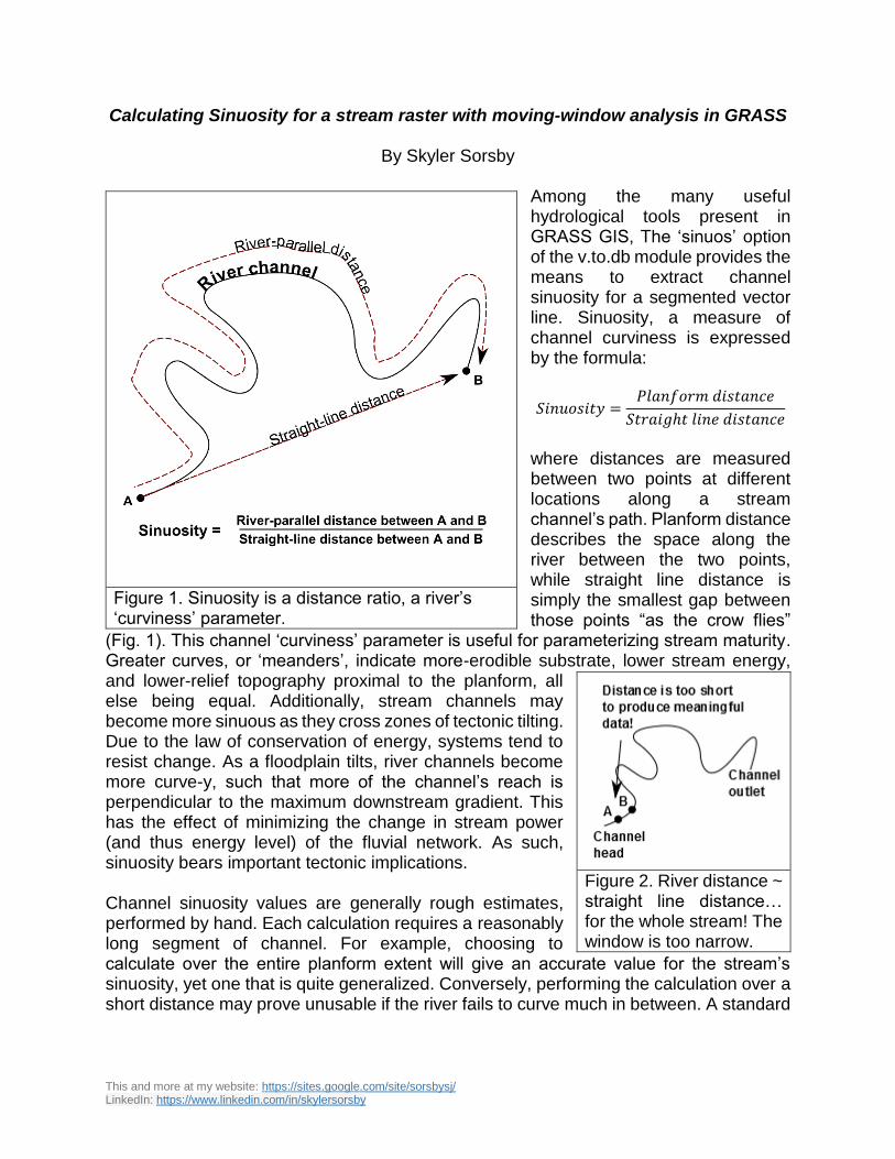
Among the many useful hydrological tools present in GRASS GIS, The ‘sinuos’ option of the v.to.db module provides the means to extract channel sinuosity for a segmented vector line. Sinuosity, a measure of channel curviness is expressed by the formula:

𝑆𝑖𝑛𝑢𝑜𝑠𝑖𝑡𝑦 =𝑃𝑙𝑎𝑛𝑓𝑜𝑟𝑚 𝑑𝑖𝑠𝑡𝑎𝑛𝑐𝑒

𝑆𝑡𝑟𝑎𝑖𝑔ℎ𝑡 𝑙𝑖𝑛𝑒 𝑑𝑖𝑠𝑡𝑎𝑛𝑐𝑒

where distances are measured between two points at different locations along a stream channel’s path. Planform distance describes the space along the river between the two points, while straight line distance is simply the smallest gap between those points “as the crow flies”

(Fig. 1). This channel ‘curviness’ parameter is useful for parameterizing stream maturity. Greater curves, or ‘meanders’, indicate more-erodible substrate, lower stream energy, and lower-relief topography proximal to the planform, all else being equal. Additionally, stream channels may become more sinuous as they cross zones of tectonic tilting. Due to the law of conservation of energy, systems tend to resist change. As a floodplain tilts, river channels become more curve-y, such that more of the channel’s reach is perpendicular to the maximum downstream gradient. This has the effect of minimizing the change in stream power (and thus energy level) of the fluvial network. As such, sinuosity bears important tectonic implications. Channel sinuosity values are generally rough estimates, performed by hand. Each calculation requires a reasonably long segment of channel. For example, choosing to calculate over the entire planform extent will give an accurate value for the stream’s sinuosity, yet one that is quite generalized. Conversely, performing the calculation over a short distance may prove unusable if the river fails to curve much in between. A standard

Figure 1. Sinuosity is a distance ratio, a river’s ‘curviness’ parameter.

Figure 2. River distance ~ straight line distance… for the whole stream! The window is too narrow.

https://sites.google.com/site/sorsbysj/

https://www.linkedin.com/in/skylersorsby


compromise is to measure over a distance equal to one (or one-half) wavelength of the river’s general periodic curve. One problem with making a single calculation over a segment of a river, however, is that it treats change in a discrete manner. Planform geometry, however, varies gradationally along a river’s course. Accordingly, sinuosity measurements, although dependent on adjacent upstream and downstream portions of a river, must be calculated in a way that shows gradational change. My proposed solution to this problem is to utilize a sufficiently long moving-window for each downstream step. With this approach, higher-resolution, continuous sinuosity is calculated over a representative, wavelength-scale reach surrounding each pixel in a stream raster. Here, I offer for review a new method for digitally calculating channel sinuosity, using the r.mapcalc, r.stream.distance, and r.neighbors GRASS modules. Additionally, I provide the Python code to perform this calculation in an automated GRASS script.

Sinuosity Workflow:

*NOTE: this workflow requires the freely-accessible r.stream.distance GRASS Addon* (Obtain r.stream distance from SettingsAddons extensions g.extention)

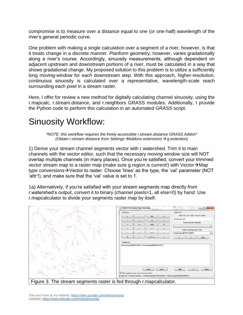
1) Derive your stream channel segments vector with r.watershed. Trim it to main channels with the vector editor, such that the necessary moving window size will NOT overlap multiple channels (in many places). Once you’re satisfied, convert your trimmed vector stream map to a raster map (make sure g.region is current!) with VectorMap type conversionsVector to raster. Choose ‘lines’ as the type, the ‘val’ parameter (NOT ‘attr’!), and make sure that the ‘val’ value is set to 1. 1a) Alternatively, if you’re satisfied with your stream segments map directly from r.watershed’s output, convert it to binary (channel pixels=1, all else=0) by hand: Use r.mapcalculator to divide your segments raster map by itself.

Figure 3. The stream segments raster is fed through r.mapcalculator.




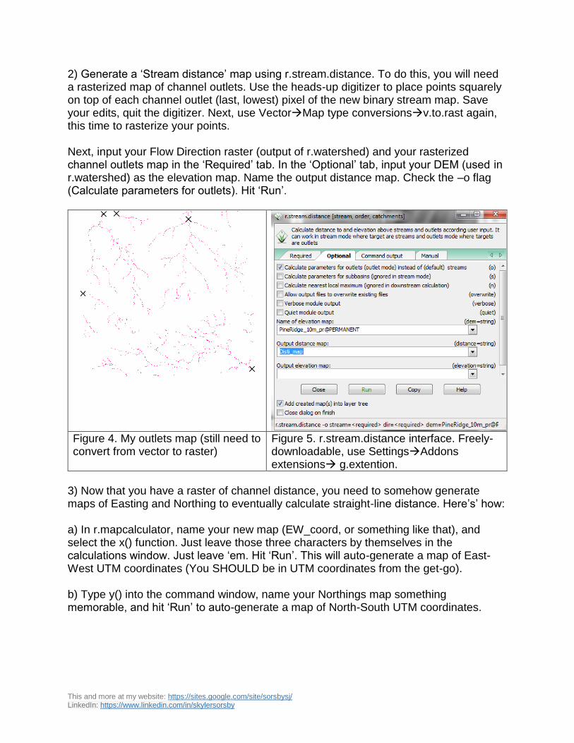
2) Generate a ‘Stream distance’ map using r.stream.distance. To do this, you will need a rasterized map of channel outlets. Use the heads-up digitizer to place points squarely on top of each channel outlet (last, lowest) pixel of the new binary stream map. Save your edits, quit the digitizer. Next, use VectorMap type conversionsv.to.rast again, this time to rasterize your points. Next, input your Flow Direction raster (output of r.watershed) and your rasterized channel outlets map in the ‘Required’ tab. In the ‘Optional’ tab, input your DEM (used in r.watershed) as the elevation map. Name the output distance map. Check the –o flag (Calculate parameters for outlets). Hit ‘Run’.

Figure 4. My outlets map (still need to convert from vector to raster)

Figure 5. r.stream.distance interface. Freely-downloadable, use SettingsAddons extensions g.extention.

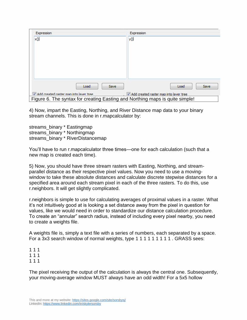
3) Now that you have a raster of channel distance, you need to somehow generate maps of Easting and Northing to eventually calculate straight-line distance. Here’s’ how: a) In r.mapcalculator, name your new map (EW_coord, or something like that), and select the x() function. Just leave those three characters by themselves in the calculations window. Just leave ‘em. Hit ‘Run’. This will auto-generate a map of East-West UTM coordinates (You SHOULD be in UTM coordinates from the get-go). b) Type y() into the command window, name your Northings map something memorable, and hit ‘Run’ to auto-generate a map of North-South UTM coordinates.




Figure 6. The syntax for creating Easting and Northing maps is quite simple!

4) Now, impart the Easting, Northing, and River Distance map data to your binary stream channels. This is done in r.mapcalculator by: streams_binary * Eastingmap streams_binary * Northingmap streams_binary * RiverDistancemap You’ll have to run r.mapcalculator three times—one for each calculation (such that a new map is created each time). 5) Now, you should have three stream rasters with Easting, Northing, and stream-parallel distance as their respective pixel values. Now you need to use a moving-window to take these absolute distances and calculate discrete stepwise distances for a specified area around each stream pixel in each of the three rasters. To do this, use r.neighbors. It will get slightly complicated. r.neighbors is simple to use for calculating averages of proximal values in a raster. What it’s not intuitively good at is looking a set distance away from the pixel in question for values, like we would need in order to standardize our distance calculation procedure. To create an “annular” search radius, instead of including every pixel nearby, you need to create a weights file. A weights file is, simply a text file with a series of numbers, each separated by a space. For a 3x3 search window of normal weights, type 1 1 1 1 1 1 1 1 1 . GRASS sees: 1 1 1 1 1 1 1 1 1 The pixel receiving the output of the calculation is always the central one. Subsequently, your moving-average window MUST always have an odd width! For a 5x5 hollow




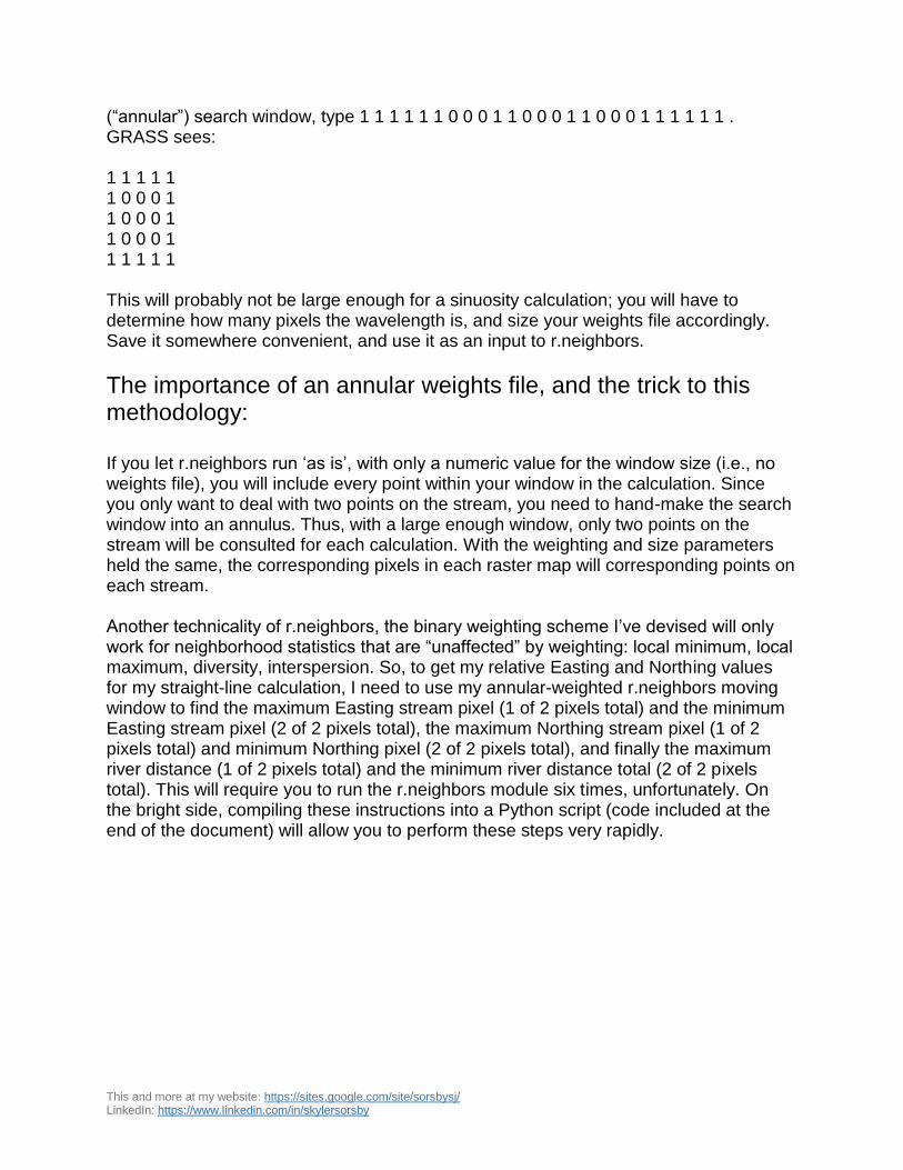
(“annular”) search window, type 1 1 1 1 1 1 0 0 0 1 1 0 0 0 1 1 0 0 0 1 1 1 1 1 1 . GRASS sees: 1 1 1 1 1 1 0 0 0 1 1 0 0 0 1 1 0 0 0 1 1 1 1 1 1 This will probably not be large enough for a sinuosity calculation; you will have to determine how many pixels the wavelength is, and size your weights file accordingly. Save it somewhere convenient, and use it as an input to r.neighbors.

The importance of an annular weights file, and the trick to this methodology: If you let r.neighbors run ‘as is’, with only a numeric value for the window size (i.e., no weights file), you will include every point within your window in the calculation. Since you only want to deal with two points on the stream, you need to hand-make the search window into an annulus. Thus, with a large enough window, only two points on the stream will be consulted for each calculation. With the weighting and size parameters held the same, the corresponding pixels in each raster map will corresponding points on each stream. Another technicality of r.neighbors, the binary weighting scheme I’ve devised will only work for neighborhood statistics that are “unaffected” by weighting: local minimum, local maximum, diversity, interspersion. So, to get my relative Easting and Northing values for my straight-line calculation, I need to use my annular-weighted r.neighbors moving window to find the maximum Easting stream pixel (1 of 2 pixels total) and the minimum Easting stream pixel (2 of 2 pixels total), the maximum Northing stream pixel (1 of 2 pixels total) and minimum Northing pixel (2 of 2 pixels total), and finally the maximum river distance (1 of 2 pixels total) and the minimum river distance total (2 of 2 pixels total). This will require you to run the r.neighbors module six times, unfortunately. On the bright side, compiling these instructions into a Python script (code included at the end of the document) will allow you to perform these steps very rapidly.




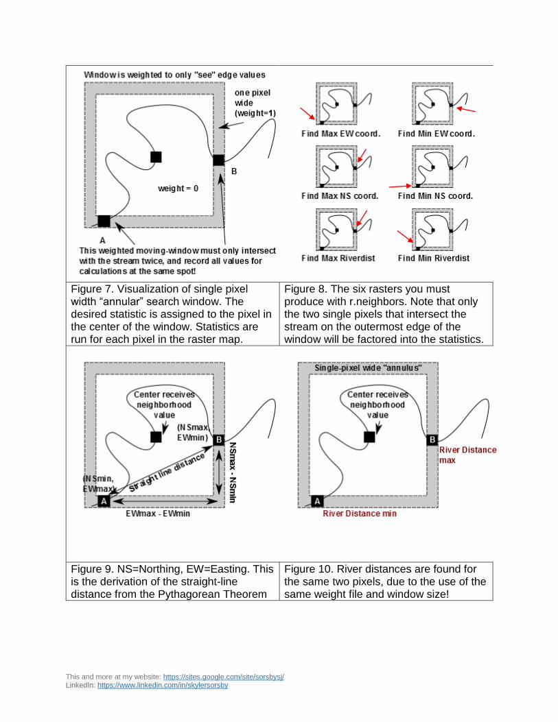
Figure 7. Visualization of single pixel width “annular” search window. The desired statistic is assigned to the pixel in the center of the window. Statistics are run for each pixel in the raster map.

Figure 8. The six rasters you must produce with r.neighbors. Note that only the two single pixels that intersect the stream on the outermost edge of the window will be factored into the statistics.

Figure 9. NS=Northing, EW=Easting. This is the derivation of the straight-line distance from the Pythagorean Theorem

Figure 10. River distances are found for the same two pixels, due to the use of the same weight file and window size!




6) Now, you should have six output maps, containing max and min Northing, max and

min Easting, and max and min river distances for corresponding pixels in each stream

raster. The problem now, is, the stream lines are suddenly quite thick! Remember that

r.neighbors acts upon each cell within the raster—if any of the zero-value cells sees a

stream cell intersecting its “annular” search window, it will nab that stream cell’s value.

Don’t worry—this doesn’t affect the stream cells. We haven’t run multiple iterations.

The fix is simple: multiply each output map by your binary stream map (1’s and 0’s) to

extract Northings, Eastings, and stream distances for only stream pixels.

7) Now, use some fancy map algebra and the Pythagorean Theorem to derive a

straight-line distance for each pixel in the study area:

sqrt( (EastingMax – EastingMin)^2 + (NorthingMax – NorthingMin)^2 )

NOTE: this is too complex for Python scripting, and requires “Expert mode”. I reduce its

complexity instead by removing the squaring notation:

sqrt( (EastingMax – EastingMin)* (EastingMax – EastingMin) + (NorthingMax – NorthingMin)* (NorthingMax – NorthingMin) )

8) Use less-fancy map algebra to derive stream distance for each pixel in the study

area:

StreamDistanceMax – StreamDistanceMin

9) Finally, use Map Algebra to divide StreamDistance by StraighLineDistance:

StreamDistance / StraightLineDistance

And, voila! You have sinuosity calculated over a desired moving window for each pixel

in your stream system, no manual calculations required. Although no more

representative than calculating sinuosity for set blocks of vector stream segments with

v.to.db, this approach may produce results that are more easily-manipulated and useful

to work with!




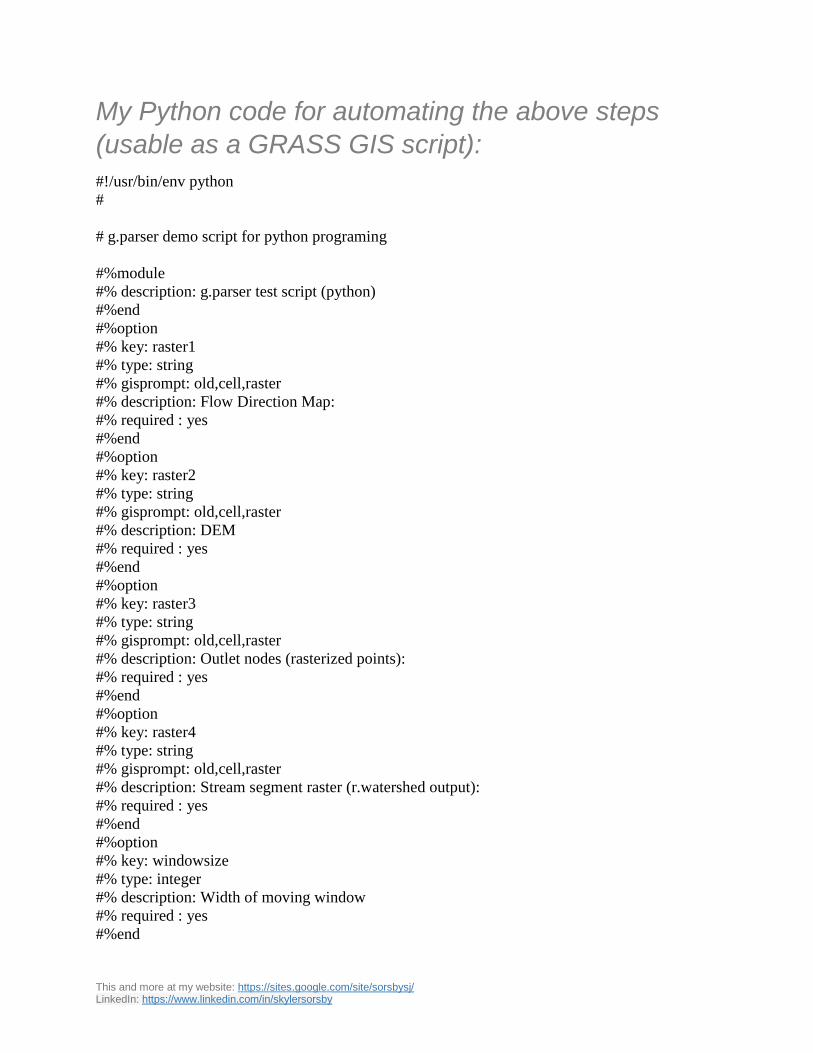
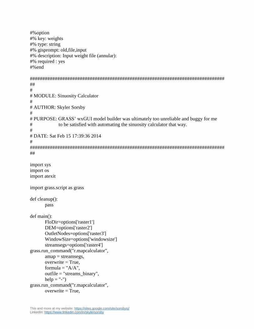
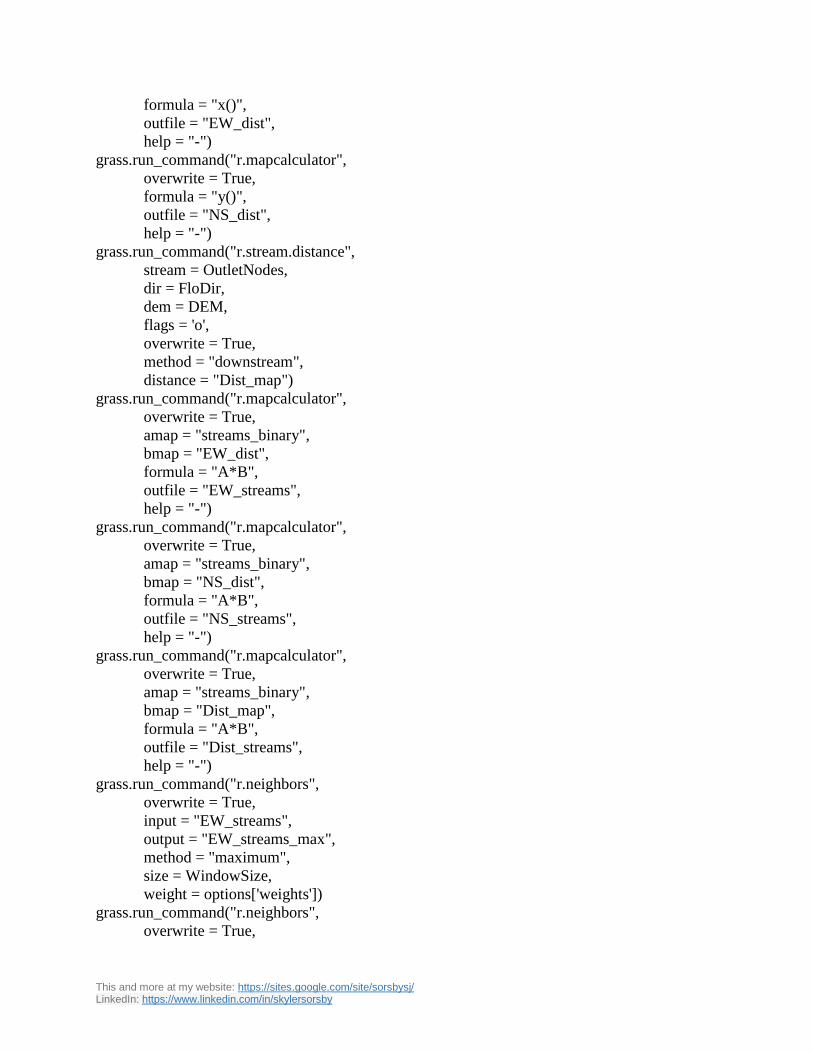
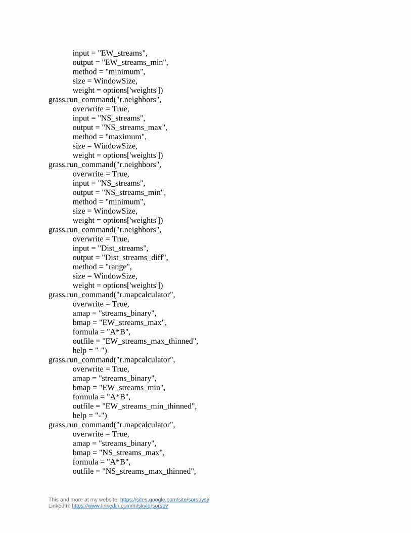
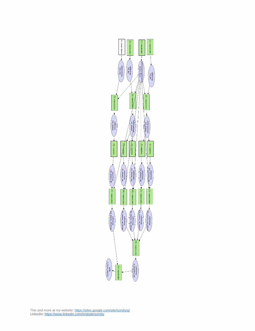
My Python code for automating the above steps

(usable as a GRASS GIS script):

#!/usr/bin/env python

#

# g.parser demo script for python programing

#%module

#% description: g.parser test script (python)

#%end

#%option

#% key: raster1

#% type: string

#% gisprompt: old,cell,raster

#% description: Flow Direction Map:

#% required : yes

#%end

#%option

#% key: raster2

#% type: string


#% description: DEM

#% required : yes

#%end

#%option

#% key: raster3

#% type: string


#% description: Outlet nodes (rasterized points):

#% required : yes

#%end

#%option

#% key: raster4

#% type: string


#% description: Stream segment raster (r.watershed output):

#% required : yes

#%end

#%option

#% key: windowsize

#% type: integer

#% description: Width of moving window

#% required : yes

#%end




#%option

#% key: weights

#% type: string

#% gisprompt: old,file,input

#% description: Input weight file (annular):

#% required : yes

#%end

##############################################################################

##

#

# MODULE: Sinuosity Calculator

#

# AUTHOR: Skyler Sorsby

#

# PURPOSE: GRASS’ wxGUI model builder was ultimately too unreliable and buggy for me

# to be satisfied with automating the sinuosity calculator that way.

#

# DATE: Sat Feb 15 17:39:36 2014

#

##############################################################################

##

import sys

import os

import atexit

import grass.script as grass

def cleanup():

pass

def main():

FloDir=options['raster1']

DEM=options['raster2']

OutletNodes=options['raster3']

WindowSize=options['windowsize']

streamsegs=options['raster4']

grass.run_command("r.mapcalculator",

amap = streamsegs,

overwrite = True,

formula = "A/A",

outfile = "streams_binary",

help = "-")


overwrite = True,




formula = "x()",

outfile = "EW_dist",

help = "-")


overwrite = True,

formula = "y()",

outfile = "NS_dist",

help = "-")

grass.run_command("r.stream.distance",

stream = OutletNodes,

dir = FloDir,

dem = DEM,

flags = 'o',

overwrite = True,

method = "downstream",

distance = "Dist_map")


overwrite = True,

amap = "streams_binary",

bmap = "EW_dist",

formula = "A*B",

outfile = "EW_streams",

help = "-")


overwrite = True,


bmap = "NS_dist",

formula = "A*B",

outfile = "NS_streams",

help = "-")


overwrite = True,


bmap = "Dist_map",

formula = "A*B",

outfile = "Dist_streams",

help = "-")

grass.run_command("r.neighbors",

overwrite = True,

input = "EW_streams",

output = "EW_streams_max",

method = "maximum",

size = WindowSize,

weight = options['weights'])


overwrite = True,




input = "EW_streams",

output = "EW_streams_min",

method = "minimum",

size = WindowSize,



overwrite = True,

input = "NS_streams",

output = "NS_streams_max",

method = "maximum",

size = WindowSize,



overwrite = True,

input = "NS_streams",

output = "NS_streams_min",

method = "minimum",

size = WindowSize,



overwrite = True,

input = "Dist_streams",

output = "Dist_streams_diff",

method = "range",

size = WindowSize,



overwrite = True,


bmap = "EW_streams_max",

formula = "A*B",

outfile = "EW_streams_max_thinned",

help = "-")


overwrite = True,


bmap = "EW_streams_min",

formula = "A*B",

outfile = "EW_streams_min_thinned",

help = "-")


overwrite = True,


bmap = "NS_streams_max",

formula = "A*B",

outfile = "NS_streams_max_thinned",




help = "-")


overwrite = True,


bmap = "NS_streams_min",

formula = "A*B",

outfile = "NS_streams_min_thinned",

help = "-")


overwrite = True,


bmap = "Dist_streams_diff",

formula = "A*B",

outfile = "Dist_streams_diff_thinned",

help = "-")


overwrite = True,

amap = "EW_streams_max_thinned",

bmap = "EW_streams_min_thinned",

cmap = "NS_streams_max_thinned",

dmap = "NS_streams_min_thinned",

formula = "sqrt((A-B)*(A-B)+(C-D)*(C-D))",

outfile = "A_straightline_dist",

help = "-")


overwrite = True,

amap = "Dist_streams_diff_thinned",

bmap = "A_straightline_dist",

formula = "A/B",

outfile = "A_stream_sinuosity",

help = "-")

return 0

if __name__ == "__main__":

options, flags = grass.parser()

atexit.register(cleanup)

sys.exit(main())






Science

Calculation of sinuosity in GRASS GIS