Embed Size (px)
Citation preview

Hydrological modeling of coupled surface-subsurfaceflow and transport phenomena: the
CATchment-HYdrology Flow-Transport (CATHY_FT)model
Workshop on coupled hydrological modeling
Carlotta Scudeler, Claudio Paniconi, Mario Putti
Padua, 23-09-2015

�� ��INTRODUCTION CATHY_FT MODEL PERFORMANCE
Many challenges in improving and testing current state-of-the-artmodels for integrated hydrological simulation
Not so many models address both flow and transport interactionsbetween the subsurface and surface
I am presenting the CATchment-HYdrology Flow-Transportmodel and I am showing its performance under hillslopedrainage, seepage face, and runoff generation
C Scudeler Padua Workshop, Padua, 23-09-2015 2/17

II. CATchment HYdrology Flow
and Transport model

INTRODUCTION�� ��CATHY_FT MODEL PERFORMANCE
CATchment HYdrology (CATHY) model
Sw Ss∂ψ∂t + φ∂Sw
∂t = −∇ · q + qss
∂Q∂t + ck
∂Q∂s = Dh
∂2Q∂s2 + ck qs
∂θc∂t = ∇ · [−qc + D∇c] + qtss
∂Qm∂t + ct
∂Qm∂s = Dc
∂2Qm∂s2 + ctqts
C Scudeler Padua Workshop, Padua, 23-09-2015 4/17

INTRODUCTION�� ��CATHY_FT MODEL PERFORMANCE
CATHY Flow-Transport (CATHY_FT) model
Sw Ss∂ψ∂t + φ∂Sw
∂t = −∇ · q + qss
∂Q∂t + ck
∂Q∂s = Dh
∂2Q∂s2 + ck qs
∂θc∂t = ∇ · [−qc + D∇c] + qtss
∂Qm∂t + ct
∂Qm∂s = Dc
∂2Qm∂s2 + ctqts
C Scudeler Padua Workshop, Padua, 23-09-2015 5/17

INTRODUCTION�� ��CATHY_FT MODEL PERFORMANCE
Numerical model
Richards’ equation (subsurface flow)
Sw Ss∂ψ∂t + φ∂Sw
∂t = −∇ · q + qss
∂Q∂t + ck
∂Q∂s = Dh
∂2Q∂s2 + ck qs
∂θc∂t = ∇ · [−qc + D∇c] + qtss
∂Qm∂t + ct
∂Qm∂s = Dc
∂2Qm∂s2 + ctqts
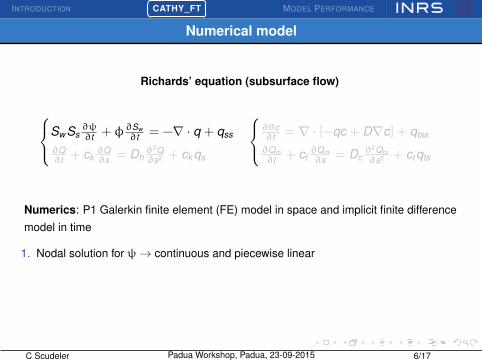
Numerics: P1 Galerkin finite element (FE) model in space and implicit finite differencemodel in time
1. Nodal solution for ψ→ continuous and piecewise linear
2. Elementwise post-computation of the velocity field q from direct application ofDarcy’s law→ elementwise constant, normal flux discontinous and notmass-conservative across every face
3. Larson-Niklasson (LN) velocity field q reconstruction
C Scudeler Padua Workshop, Padua, 23-09-2015 6/17
INTRODUCTION�� ��CATHY_FT MODEL PERFORMANCE
Numerical model
Richards’ equation (subsurface flow)
Sw Ss∂ψ∂t + φ∂Sw
∂t = −∇ · q + qss
∂Q∂t + ck
∂Q∂s = Dh
∂2Q∂s2 + ck qs
∂θc∂t = ∇ · [−qc + D∇c] + qtss
∂Qm∂t + ct
∂Qm∂s = Dc
∂2Qm∂s2 + ctqts
Numerics: P1 Galerkin finite element (FE) model in space and implicit finite differencemodel in time
1. Nodal solution for ψ→ continuous and piecewise linear
2. Elementwise post-computation of the velocity field q from direct application ofDarcy’s law→ elementwise constant, normal flux discontinous and notmass-conservative across every face
3. Larson-Niklasson (LN) velocity field q reconstruction
C Scudeler Padua Workshop, Padua, 23-09-2015 6/17

INTRODUCTION�� ��CATHY_FT MODEL PERFORMANCE
Numerical model
ADE equation (subsurface transport)
Sw Ss∂ψ∂t + φ∂Sw
∂t = −∇ · q + qss
∂Q∂t + ck
∂Q∂s = Dh
∂2Q∂s2 + ck qs
∂θc∂t = ∇ · [−qc + D∇c] + qtss
∂Qm∂t + ct
∂Qm∂s = Dc
∂2Qm∂s2 + ctqts
Numerics: High resolution finite volume (for -∇ · qc advective step) and FE (for∇ · (D∇c) dispersive step) combined with a time-splitting technique
1. Advective time-explicit step for the elementwise c
2. Mass-conservative element→node c reconstruction
3. Dispersive time-implicit step for the nodal c
4. Mass-conservative node→element c reconstruction
C Scudeler Padua Workshop, Padua, 23-09-2015 6/17

INTRODUCTION�� ��CATHY_FT MODEL PERFORMANCE
Numerical model
Surface flow and transport equations
Sw Ss∂ψ∂t + φ∂Sw
∂t = −∇ · q + qss
∂Q∂t + ck
∂Q∂s = Dh
∂2Q∂s2 + ck qs
∂θc∂t = ∇ · [−qc + D∇c] + qtss
∂Qm∂t + ct
∂Qm∂s = Dc
∂2Qm∂s2 + ctqts
Numerics: Explicit finite difference scheme in space and time for both surface flow andtransport solution
C Scudeler Padua Workshop, Padua, 23-09-2015 6/17

INTRODUCTION�� ��CATHY_FT MODEL PERFORMANCE
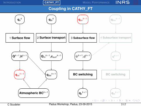
Coupling in CATHY_FT
1 Surface flow 2 Surface transport 3 Subsurface flow 4 Subsurface transport
qsk qts
k
Qk+1,hk+1 Qmk+1,csurf
k+1 ψk+1,qk+1
BC switching
ck+1
BC switchingqssk+1
Atmospheric BCk+1
qssk+1
qtssk+1
qtssk+1
qsk+1 qts
k+1
C Scudeler Padua Workshop, Padua, 23-09-2015 7/17

INTRODUCTION�� ��CATHY_FT MODEL PERFORMANCE
Coupling in CATHY_FT
1 Surface flow 2 Surface transport 3 Subsurface flow 4 Subsurface transport
qsk qts
k
Qk+1,hk+1 Qmk+1,csurf
k+1 ψk+1,qk+1
BC switching
Atmospheric BCk+1
ck+1
BC switchingqssk+1
qssk+1
qtssk+1
qtssk+1
qsk+1 qts
k+1
C Scudeler Padua Workshop, Padua, 23-09-2015 7/17
INTRODUCTION�� ��CATHY_FT MODEL PERFORMANCE
Coupling in CATHY_FT
1 Surface flow 2 Surface transport 3 Subsurface flow 4 Subsurface transport
qsk qts
k
Qk+1,hk+1 Qmk+1,csurf
k+1
Atmospheric BCk+1
ψk+1,qk+1
BC switching
ck+1
BC switchingqssk+1
qssk+1
qtssk+1
qtssk+1
qsk+1 qts
k+1
C Scudeler Padua Workshop, Padua, 23-09-2015 7/17

INTRODUCTION�� ��CATHY_FT MODEL PERFORMANCE
Coupling in CATHY_FT
1 Surface flow 2 Surface transport 3 Subsurface flow 4 Subsurface transport
qsk qts
k
Qk+1,hk+1
Atmospheric BCk+1
Qmk+1,csurf
k+1 ψk+1,qk+1
BC switching
ck+1
BC switchingqssk+1
qssk+1
qtssk+1
qtssk+1
qsk+1 qts
k+1
C Scudeler Padua Workshop, Padua, 23-09-2015 7/17

INTRODUCTION�� ��CATHY_FT MODEL PERFORMANCE
Coupling in CATHY_FT
1 Surface flow 2 Surface transport 3 Subsurface flow
Atmospheric BCk+1
4 Subsurface transport
qsk qts
k
Qk+1,hk+1 Qmk+1,csurf
k+1 ψk+1,qk+1
BC switching
ck+1
BC switchingqssk+1
qssk+1
qtssk+1
qtssk+1
qsk+1 qts
k+1
C Scudeler Padua Workshop, Padua, 23-09-2015 7/17

INTRODUCTION�� ��CATHY_FT MODEL PERFORMANCE
Model accuracy
Ability of the model to conserve mass
C Scudeler Padua Workshop, Padua, 23-09-2015 8/17

INTRODUCTION�� ��CATHY_FT MODEL PERFORMANCE
Model accuracy
Ability of the model to conserve mass
Sw Ss∂ψ
∂t+ φ
∂Sw
∂t= −∇ · q + qss
→Mass-conservative solutionachieved solving the equation inits ψ− Sw mixed form [Celia et al.,1990]
C Scudeler Padua Workshop, Padua, 23-09-2015 8/17

INTRODUCTION�� ��CATHY_FT MODEL PERFORMANCE
Model accuracy
Ability of the model to conserve mass
∂θc∂t
= ∇ · [−qc + D∇c] + qtss→
HRFV mass-conservative solutionif q is mass-conservative.
C Scudeler Padua Workshop, Padua, 23-09-2015 8/17

INTRODUCTION�� ��CATHY_FT MODEL PERFORMANCE
Model accuracy
Ability of the model to conserve mass
∂θc∂t
= ∇ · [−qc + D∇c] + qtss→
HRFV mass-conservative solutionif q is mass-conservative.P1 Galerkin q is notmass-conservative
C Scudeler Padua Workshop, Padua, 23-09-2015 8/17

INTRODUCTION�� ��CATHY_FT MODEL PERFORMANCE
Model accuracy
Ability of the model to conserve mass
∂θc∂t
= ∇ · [−qc + D∇c] + qtss→
HRFV mass-conservative solutionif q is mass-conservative.P1 Galerkin q is notmass-conservative
To make q mass-conservative:
change the numerical scheme from FE =⇒ High computational costto Mixed Hybrid Finite Element (MHFE)
or
add mass-conservative velocity field =⇒ Low computational costreconstruction
In CATHY_FT: FE =⇒ FE+Larson-Niklasson (LN) post-processing technique
C Scudeler Padua Workshop, Padua, 23-09-2015 8/17

INTRODUCTION�� ��CATHY_FT MODEL PERFORMANCE
Larson-Niklasson technique
Domain discretized by ne tetrahedral elements and n nodes
At each time step
qe is the non mass-conservative element velocity
Rei is the element residual associated to each node i
~n is the vector normal to each element faces
qeLN is the mass-conservative element velocity
C Scudeler Padua Workshop, Padua, 23-09-2015 9/17

INTRODUCTION�� ��CATHY_FT MODEL PERFORMANCE
Larson-Niklasson technique
Domain discretized by ne tetrahedral elements and n nodes
At each time step
CATHY solution
· ψ nodal solution· qe non mass-conservative
where:qe is the non mass-conservative element velocity
Rei is the element residual associated to each node i
~n is the vector normal to each element faces
qeLN is the mass-conservative element velocity
C Scudeler Padua Workshop, Padua, 23-09-2015 9/17

INTRODUCTION�� ��CATHY_FT MODEL PERFORMANCE
Larson-Niklasson technique
Domain discretized by ne tetrahedral elements and n nodes
At each time step
CATHY solution
· ψ nodal solution· qe non mass-conservative
· Rei
· ~q·~n
where:qe is the non mass-conservative element velocity
Rei is the element residual associated to each node i
~n is the vector normal to each element faces
qeLN is the mass-conservative element velocity
C Scudeler Padua Workshop, Padua, 23-09-2015 9/17

INTRODUCTION�� ��CATHY_FT MODEL PERFORMANCE
Larson-Niklasson technique
Domain discretized by ne tetrahedral elements and n nodes
At each time step
CATHY solution
· ψ nodal solution· qe non mass-conservative
· Rei
· ~q·~n Larson-Niklasson
· new ~qLN ·~n· new mass-conservative qe
LN
where:qe is the non mass-conservative element velocity
Rei is the element residual associated to each node i
~n is the vector normal to each element faces
qeLN is the mass-conservative element velocity
C Scudeler Padua Workshop, Padua, 23-09-2015 9/17

INTRODUCTION�� ��CATHY_FT MODEL PERFORMANCE
LN velocity reconstruction results
1. Convergent streamlines towards an outlet
2. High streamline curvatures due to heterogeneity
C Scudeler Padua Workshop, Padua, 23-09-2015 10/17

INTRODUCTION�� ��CATHY_FT MODEL PERFORMANCE
LN velocity reconstruction results
1. Convergent streamlines towards an outlet
D=50 mD=0 m
qN=0 m/scin=1
C Scudeler Padua Workshop, Padua, 23-09-2015 10/17

INTRODUCTION�� ��CATHY_FT MODEL PERFORMANCE
LN velocity reconstruction results
1. Convergent streamlines towards an outlet
0 1 2 3 4Time (h)
25
50
75
100
Mass(%)
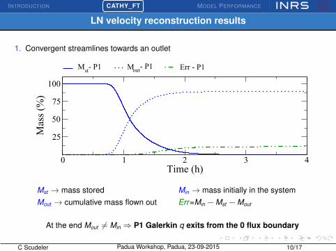
Mst- P1 Mout- P1 Err - P1
Mst → mass storedMout → cumulative mass flown out
Min → mass initially in the systemErr=Min − Mst − Mout
C Scudeler Padua Workshop, Padua, 23-09-2015 10/17
INTRODUCTION�� ��CATHY_FT MODEL PERFORMANCE
LN velocity reconstruction results
1. Convergent streamlines towards an outlet
0 1 2 3 4Time (h)
25
50
75
100
Mass(%)
Mst- P1 Mout- P1 Err - P1
Mst → mass storedMout → cumulative mass flown out
Min → mass initially in the systemErr=Min − Mst − Mout
At the end Mout 6= Min ⇒ P1 Galerkin q exits from the 0 flux boundary
C Scudeler Padua Workshop, Padua, 23-09-2015 10/17

INTRODUCTION�� ��CATHY_FT MODEL PERFORMANCE
LN velocity reconstruction results
1. Convergent streamlines towards an outlet
0 1 2 3 4Time (h)
25
50
75
100
Mass(%)
Mst- LN M
out- LN
C Scudeler Padua Workshop, Padua, 23-09-2015 10/17

INTRODUCTION�� ��CATHY_FT MODEL PERFORMANCE
LN velocity reconstruction results
1. Convergent streamlines towards an outlet
0 1 2 3 4Time (h)
25
50
75
100
Mass(%)
Mst- LN M
out- LN
Velocities reconstructed with LN do not violate the 0 flux boundaries
C Scudeler Padua Workshop, Padua, 23-09-2015 10/17

INTRODUCTION�� ��CATHY_FT MODEL PERFORMANCE
LN velocity reconstruction results
1. Convergent streamlines towards an outlet
2. High streamline curvatures due to heterogeneity
D=50 mD=0 m
qN=0 m/scin=1
Ks (m/s)2x10-4
2x10-12
C Scudeler Padua Workshop, Padua, 23-09-2015 11/17

INTRODUCTION�� ��CATHY_FT MODEL PERFORMANCE
LN velocity reconstruction results
1. Convergent streamlines towards an outlet
2. High streamline curvatures due to heterogeneity
0 2 4 6 8 10Time (h)
Mst- LN M
stf- LN
0 2 4 6 8Time (h)
25
50
75
100
Mass(%)
Mst- P1 M
stf- P1
Mstf → mass stored in the unpermeable soil Mst → mass stored
At the end for P1 Mstf = Mst 6=0 ⇒ Solute mass get trapped in the unpermeable soil
At the end for LN Mstf = Mst =0 ⇒ Solute mass slightly crosses the unpermeable soil
C Scudeler Padua Workshop, Padua, 23-09-2015 11/17
III. Testing CATHY_FT at the
Landscape Evolution
Observatory (LEO)

INTRODUCTION CATHY_FT�� ��MODEL PERFORMANCE
The Landscape Evolution Observatory (LEO)
LEO, Biosphere 2, Oracle,Arizona, U.S.A.
3 convergent landscapes30 m long, 11.5 m wide
dense sensor and samplernetwork
rainfall simulator (3-45mm/h)
View of one of the threehillslopes from top
Tipping bucket for low seepageface flow
Rainfall simulator
C Scudeler Padua Workshop, Padua, 23-09-2015 13/17

INTRODUCTION CATHY_FT�� ��MODEL PERFORMANCE
The Landscape Evolution Observatory (LEO)
LEO, Biosphere 2, Oracle,Arizona, U.S.A.
3 convergent landscapes30 m long, 11.5 m wide
dense sensor and samplernetwork
rainfall simulator (3-45mm/h)
In Figure:
View of one of the threehillslopes from top
Tipping bucket for low seepageface flow
Rainfall simulator
C Scudeler Padua Workshop, Padua, 23-09-2015 13/17

INTRODUCTION CATHY_FT�� ��MODEL PERFORMANCE
Test case
Computational domain60 x 22 grid cells
30 layers; more refined close to thesurface and at bottom
C Scudeler Padua Workshop, Padua, 23-09-2015 14/17

INTRODUCTION CATHY_FT�� ��MODEL PERFORMANCE
Test case
Computational domain60 x 22 grid cells
30 layers; more refined close to thesurface and at bottom
Material model:
homogeneity with Ks=1×10⁻⁴ m/sand φ=0.39
Van Genuchten parametersnVG=2.26, θres=0.002, ψsat =-0.6 m
Model performance for Subsurface-Surface flow and transport
1) Rainfall
C Scudeler Padua Workshop, Padua, 23-09-2015 14/17

INTRODUCTION CATHY_FT�� ��MODEL PERFORMANCE
Test case
Computational domain60 x 22 grid cells
30 layers; more refined close to thesurface and at bottom
Material model:
homogeneity with Ks=1×10⁻⁴ m/sand φ=0.39
Van Genuchten parametersnVG=2.26, θres=0.002, ψsat =-0.6 m
Model performance for Subsurface-Surface flow and transport
1) Rainfall2) Seepage face flow
3) Drainage under variably saturated conditions
C Scudeler Padua Workshop, Padua, 23-09-2015 14/17

INTRODUCTION CATHY_FT�� ��MODEL PERFORMANCE
Test case
Computational domain60 x 22 grid cells
30 layers; more refined close to thesurface and at bottom
Material model:
homogeneity with Ks=1×10⁻⁴ m/sand φ=0.39
Van Genuchten parametersnVG=2.26, θres=0.002, ψsat =-0.6 m
Model performance for Subsurface-Surface flow and transport
1) Rainfall2) Seepage face flow
3) Drainage under variably saturated conditions4) Surface flow
C Scudeler Padua Workshop, Padua, 23-09-2015 14/17

INTRODUCTION CATHY_FT�� ��MODEL PERFORMANCE
Test case
Seepage Face
Outlet
Computational domain60 x 22 grid cells
30 layers; more refined close to thesurface and at bottom
Material model:
homogeneity with Ks=1×10⁻⁴ m/sand φ=0.39
Van Genuchten parametersnVG=2.26, θres=0.002, ψsat =-0.6 m
Model performance for Subsurface-Surface flow and transport
1) Rainfall2) Seepage face flow
3) Drainage under variably saturated conditions4) Surface flow
C Scudeler Padua Workshop, Padua, 23-09-2015 14/17

INTRODUCTION CATHY_FT�� ��MODEL PERFORMANCE
Input
Water and solute mass inflow Cumulative volume and mass
0.005
0.01
0.015
Qr(m
3 /s)
0 6 12 18 24 30 36 42 48Time (h)
0.005
0.01
0.015
Qm(mg/s)
15
30
45
60
Vr(m
3 )
0 6 12 18 24 30 36 42 48Time (h)
15
30
45
60
Min(mg)
Initial conditions: 119 m3 of water initially present in the system (water table set at 0.4 mfrom bottom) and 0 solute mass
Flow input : pulse of homogenous rain Qr =0.012 m3/s for 1 h→ cumulative volumeinjected Vr =40.4 m3
Transport input : solute injection with c=1 mg/m3 of rain pulse→ mass inflow Qm=0.012mg/s and cumulative mass injected Min=40.4 mg
C Scudeler Padua Workshop, Padua, 23-09-2015 15/17

INTRODUCTION CATHY_FT�� ��MODEL PERFORMANCE
Input
Water and solute mass inflow Cumulative volume and mass
0.005
0.01
0.015
Qr(m
3 /s)
0 6 12 18 24 30 36 42 48Time (h)
0.005
0.01
0.015
Qm(mg/s)
Qr=0.012 m3/s
15
30
45
60
Vr(m
3 )
0 6 12 18 24 30 36 42 48Time (h)
15
30
45
60
Min(mg)
Vr=40.4 m3
Initial conditions: 119 m3 of water initially present in the system (water table set at 0.4 mfrom bottom) and 0 solute mass
Flow input : pulse of homogenous rain Qr =0.012 m3/s for 1 h→ cumulative volumeinjected Vr =40.4 m3
Transport input : solute injection with c=1 mg/m3 of rain pulse→ mass inflow Qm=0.012mg/s and cumulative mass injected Min=40.4 mg
C Scudeler Padua Workshop, Padua, 23-09-2015 15/17

INTRODUCTION CATHY_FT�� ��MODEL PERFORMANCE
Input
Water and solute mass inflow Cumulative volume and mass
0.005
0.01
0.015
Qr(m
3 /s)
0 6 12 18 24 30 36 42 48Time (h)
0.005
0.01
0.015
Qm(mg/s)Qm=0.012 mg/s
15
30
45
60
Vr(m
3 )
0 6 12 18 24 30 36 42 48Time (h)
15
30
45
60
Min(mg)
Min=40.4 mg
Initial conditions: 119 m3 of water initially present in the system (water table set at 0.4 mfrom bottom) and 0 solute mass
Flow input : pulse of homogenous rain Qr =0.012 m3/s for 1 h→ cumulative volumeinjected Vr =40.4 m3
Transport input : solute injection with c=1 mg/m3 of rain pulse→ mass inflow Qm=0.012mg/s and cumulative mass injected Min=40.4 mg
C Scudeler Padua Workshop, Padua, 23-09-2015 15/17

INTRODUCTION CATHY_FT�� ��MODEL PERFORMANCE
Results
Water balance
4080
Vr(%)
-4004080
∆Vst(%)
4080
Vsf(%)
0 6 12 18 24 30 36 42 48Time (h)
4080
Vout(%)
4080
Min(%)
10203040
∆Mst(%)
5
10
Msf(%)
0 6 12 18 24 30 36 42 48Time (h)
306090
Mout(%)
Vr − ∆Vst − Vsf − Vout = Flow Error
Min − ∆Mst − Msf − Mout = Transport Error
C Scudeler Padua Workshop, Padua, 23-09-2015 16/17

INTRODUCTION CATHY_FT�� ��MODEL PERFORMANCE
Results
Water balance
4080
Vr(%)
-4004080
∆Vst(%)
4080
Vsf(%)
0 6 12 18 24 30 36 42 48Time (h)
4080
Vout(%)
Vr=100% 4080
Min(%)
10203040
∆Mst(%)
5
10
Msf(%)
0 6 12 18 24 30 36 42 48Time (h)
306090
Mout(%)
Vr − ∆Vst − Vsf − Vout ⇒100
Min − ∆Mst − Msf − Mout = Transport Error
C Scudeler Padua Workshop, Padua, 23-09-2015 16/17

INTRODUCTION CATHY_FT�� ��MODEL PERFORMANCE
Results
Water balance
4080
Vr(%)
-4004080
∆Vst(%)
4080
Vsf(%)
0 6 12 18 24 30 36 42 48Time (h)
4080
Vout(%)
-48.17%∆Vst=
4080
Min(%)
10203040
∆Mst(%)
5
10
Msf(%)
0 6 12 18 24 30 36 42 48Time (h)
306090
Mout(%)
Vr − ∆Vst − Vsf − Vout ⇒100+48.17
Min − ∆Mst − Msf − Mout = Transport Error
C Scudeler Padua Workshop, Padua, 23-09-2015 16/17

INTRODUCTION CATHY_FT�� ��MODEL PERFORMANCE
Results
Water balance
4080
Vr(%)
-4004080
∆Vst(%)
4080
Vsf(%)
0 6 12 18 24 30 36 42 48Time (h)
4080
Vout(%)
Vsf=77.62%
4080
Min(%)
10203040
∆Mst(%)
5
10
Msf(%)
0 6 12 18 24 30 36 42 48Time (h)
306090
Mout(%)
Vr − ∆Vst − Vsf − Vout ⇒100+48.17-77.62
Min − ∆Mst − Msf − Mout = Transport Error
C Scudeler Padua Workshop, Padua, 23-09-2015 16/17

INTRODUCTION CATHY_FT�� ��MODEL PERFORMANCE
Results
Water balance
4080
Vr(%)
-4004080
∆Vst(%)
4080
Vsf(%)
0 6 12 18 24 30 36 42 48Time (h)
4080
Vout(%)
Vout=70.58%
4080
Min(%)
10203040
∆Mst(%)
5
10
Msf(%)
0 6 12 18 24 30 36 42 48Time (h)
306090
Mout(%)
Vr − ∆Vst − Vsf − Vout ⇒100+48.17-77.62-70.58=o(0.01)%
Min − ∆Mst − Msf − Mout = Transport Error
C Scudeler Padua Workshop, Padua, 23-09-2015 16/17
INTRODUCTION CATHY_FT�� ��MODEL PERFORMANCE
Results
Mass balance
4080
Vr(%)
-4004080
∆Vst(%)
4080
Vsf(%)
0 6 12 18 24 30 36 42 48Time (h)
4080
Vout(%)
4080
Min(%)
10203040
∆Mst(%)
5
10
Msf(%)
0 6 12 18 24 30 36 42 48Time (h)
306090
Mout(%)
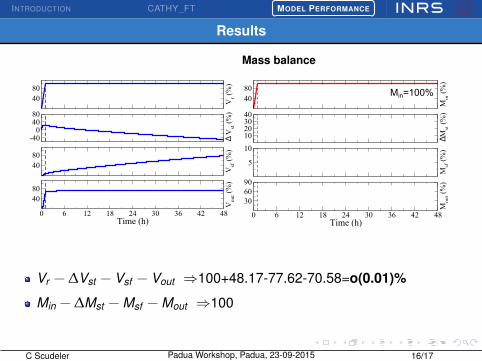
Min=100%
Vr − ∆Vst − Vsf − Vout ⇒100+48.17-77.62-70.58=o(0.01)%
Min − ∆Mst − Msf − Mout ⇒100
C Scudeler Padua Workshop, Padua, 23-09-2015 16/17

INTRODUCTION CATHY_FT�� ��MODEL PERFORMANCE
Results
Mass balance
4080
Vr(%)
-4004080
∆Vst(%)
4080
Vsf(%)
0 6 12 18 24 30 36 42 48Time (h)
4080
Vout(%)
4080
Min(%)
10203040
∆Mst(%)
5
10
Msf(%)
0 6 12 18 24 30 36 42 48Time (h)
306090
Mout(%)
∆Mst=28.62%
Vr − ∆Vst − Vsf − Vout ⇒100+48.17-77.62-70.58=o(0.01)%
Min − ∆Mst − Msf − Mout ⇒100-28.62
C Scudeler Padua Workshop, Padua, 23-09-2015 16/17
INTRODUCTION CATHY_FT�� ��MODEL PERFORMANCE
Results
Mass balance
4080
Vr(%)
-4004080
∆Vst(%)
4080
Vsf(%)
0 6 12 18 24 30 36 42 48Time (h)
4080
Vout(%)
4080
Min(%)
10203040
∆Mst(%)
5
10
Msf(%)
0 6 12 18 24 30 36 42 48Time (h)
306090
Mout(%)
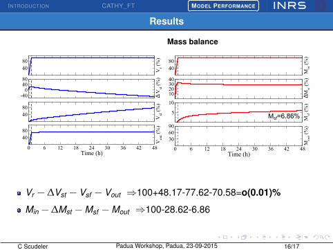
Msf=6.86%
Vr − ∆Vst − Vsf − Vout ⇒100+48.17-77.62-70.58=o(0.01)%
Min − ∆Mst − Msf − Mout ⇒100-28.62-6.86
C Scudeler Padua Workshop, Padua, 23-09-2015 16/17

INTRODUCTION CATHY_FT�� ��MODEL PERFORMANCE
Results
Mass balance
4080
Vr(%)
-4004080
∆Vst(%)
4080
Vsf(%)
0 6 12 18 24 30 36 42 48Time (h)
4080
Vout(%)
4080
Min(%)
10203040
∆Mst(%)
5
10
Msf(%)
0 6 12 18 24 30 36 42 48Time (h)
306090
Mout(%)
Mout=64.42%
Vr − ∆Vst − Vsf − Vout ⇒100+48.17-77.62-70.58=o(0.01)%
Min − ∆Mst − Msf − Mout ⇒100-28.62-6.86-64.42=o(0.1)%
C Scudeler Padua Workshop, Padua, 23-09-2015 16/17
INTRODUCTION CATHY_FT MODEL PERFORMANCE
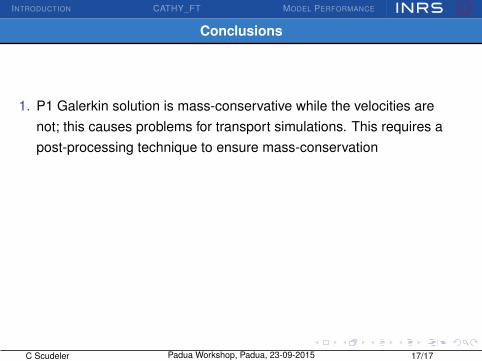
Conclusions
1. P1 Galerkin solution is mass-conservative while the velocities arenot; this causes problems for transport simulations. This requires apost-processing technique to ensure mass-conservation
2. Results so far indicate that LN reconstructed velocities are asaccurate as MHFE velocities and achieve much better computationalefficiency
3. Exchange processes in integrated surface-subsurface models arehighly complex and need to be carefully formulated and resolved
C Scudeler Padua Workshop, Padua, 23-09-2015 17/17

INTRODUCTION CATHY_FT MODEL PERFORMANCE
Conclusions
1. P1 Galerkin solution is mass-conservative while the velocities arenot; this causes problems for transport simulations. This requires apost-processing technique to ensure mass-conservation
2. Results so far indicate that LN reconstructed velocities are asaccurate as MHFE velocities and achieve much better computationalefficiency
3. Exchange processes in integrated surface-subsurface models arehighly complex and need to be carefully formulated and resolved
C Scudeler Padua Workshop, Padua, 23-09-2015 17/17

Thanks for your attention